Correction to the Casimir force due to the anomalous skin effect

Abstract

The surface impedance approach is discussed in connection with the precise calculation of the Casimir force between metallic plates. It allows to take into account the nonlocal connection between the current density and electric field inside of metals. In general, a material has to be described by two impedances $Z_{s}(\omega,q)$ and $Z_{p}(\omega,q)$ corresponding to two different polarization states. In contrast with the approximate Leontovich impedance they depend not only on frequency $\omega$ but also on the wave vector along the plate $q$. In this paper only the nonlocal effects happening at frequencies $\omega<\omega_{p}$ (plasma frequency) are analyzed. We refer to all of them as the anomalous skin effect. The impedances are calculated for the propagating and evanescent fields in the Boltzmann approximation. It is found that $Z_{p}$ significantly deviates from the local impedance as a result of the Thomas-Fermi screening. The nonlocal correction to the Casimir force is calculated at zero temperature. This correction is small but observable at small separations between bodies. The same theory can be used to find more significant nonlocal contribution at $\omega\sim\omega_{p}$ due to the plasmon excitation.

I Introduction

The Casimir force Cas between uncharged metallic plates, predicted in 1948 as a quantum electrodynamics effect, only recently became a subject of systematic experimental investigation. The reason is that nowadays with the development of microtechnologies a reliable control of the separations between bodies smaller than 1 $\mu m$ became possible. A variety of methods have been used to measure the force. In the torsion pendulum experiment Lam1 , first in the modern series, the force between a sphere and a plate covered with gold was measured with the accuracy of 5%. A significant progress was achieved in the atomic force microscope (AFM) experiments Moh1 ; Moh2 , where the sphere was attached to a cantilever. The force was deduced from the cantilever bending when the plate was approaching the sphere. In this experiment the force was measured with a 1% precision. The best result using AFM Moh2 was found when the sphere and the plate were covered with gold and special care was taken to control the surface roughness of metal. The same precision was reached in the crossed cylinders experiment Ederth , where extremely smooth gold films were used. Sophisticated microelectromechanical system (MEMS) Chan was used to measure the force between the gold plated sphere and a suspended paddle. It demonstrated the nonlinear behavior of the mechanical oscillator due to the Casimir force. The only experiment, where the force was measured in the plate-plate geometry Bressi , was done using an oscillating beam whose resonance frequency changed in response to the force. Up to date, the most precise experiment Decca1 ; Decca2 explored the MEMS device similar to that in Ref. Chan . The precision was improved due to the use of the dynamical method. Additionally the change in the resonance frequency of the mechanical oscillator was measured using the phase jump instead of resonance behavior of the amplitude. In this way the force was found with the relative accuracy of 0.25% Decca1 ; Decca2 ; Iannuzzi .

To draw any conclusion from the experiments one has to predict the force theoretically with the precision comparable with the experimental errors. In its original form, the Casimir force Cas

$$F_{c}\left(a\right)=-\frac{\pi^{2}}{240}\frac{\hbar c}{a^{4}}$$ (1)

was calculated between the ideal metals. It depends only on the fundamental constants and the distance between the plates $a$. The force between real materials, described by its dielectric functions $\varepsilon\left(\omega\right)$, was deduced for the first time by Lifshitz Lif . Corrections to Eq. (1) can be quite significant at small separation between bodies. To calculate the force with high precision the Lifshitz formula is used with the optical data taken from handbooks HB1 ; HB2 . The data are available only up to some low cut-off frequency $\omega_{cut}$. For good metals such as $Au,$ $Al,$ $Cu$ the data can be extrapolated to lower frequencies with the Drude dielectric function

$$\varepsilon\left(\omega\right)=1-\frac{\omega_{p}^{2}}{\omega\left(\omega+i\omega_{\tau}\right)},$$ (2)

which includes two parameters: the plasma frequency $\omega_{p}$ and the relaxation frequency $\omega_{\tau}$. These parameters can be extracted from the optical data at the lowest accessible frequencies. In this way the force has been calculated Lam2 ; BS0 ; LR ; SL2 ; KMM with the highest possible precision. There is some disagreement between the results of different authors connected with the choice of the relaxation frequency $\omega_{\tau}$ SL2 . This frequency can be found by fitting the low frequency optical data with Eq. (2) LR or extracted from the bulk material resistivity KMM . These details are important at small separations.

In Refs. SL1 ; SL2 it was stressed that using the handbook optical data one finds not the actual force but rather the upper limit on the Casimir force. The reason is that the handbooks comprise the data for the best samples; any material imperfection will reduce the reflectivity and, as a result, the force will be smaller. In the experiments the force is measured between the bodies covered with a metal. The metal is deposited on a substrate with the evaporation or sputtering technics Moh2 ; Decca1 . The resulting film thickness is typically in the range $100-200\,nm$. It was already noted SL1 ; SL2 that the optical properties of the films can deviate significantly from those of the bulk material. The main reasons for these deviations such as voids in the films and electron scattering on the grain boundaries were indicated recently S and the methods to estimate the effects were outlined. For the AFM Moh2 and MEMS Decca2 experiments the influence of these effects on the force was estimated on the level of 2%. Additional work from the theoretical and experimental sides has to be done to refine these estimates.

An alternative way to calculate the Casimir force using the surface impedance of metals instead of the dielectric function was discussed BKR ; SL4 ; GKM in the literature. The general formula for the Casimir force in this approach was deduced for the first time in Ref. MT . It is the same Lifshitz formula but the reflection coefficients are expressed in terms of the surface impedance. In the cited papers the approximate Leontovich impedance LL8 depending only on frequency was used. The hope was that in this approach it will be possible to resolve the long standing problem with the temperature correction to the force BS1 ; SL2 ; BGKM ; GLR ; Lam3 ; SL3 ; KM ; BAH ; HBAM . However, although the impedance approach itself seems reasonable and well motivated, the use of the approximate impedance for the Casimir force happened to be unjustified. The Leontovich impedance is well suited for the propagating photons impinging on a metal but for the Casimir problem the exact impedance has to be used since the important contribution in the force comes from the evanescent electromagnetic field. The exact impedance was shown to give the same result for the force as that in the dielectric function approach MVE .

The surface impedance is the only way to describe the interaction between the electromagnetic field and metal in the case when the relation between current and electric field in the metal becomes nonlocal. For example, at low temperatures the mean free path of the electrons in metals becomes larger than the field penetration depth, and the relation between the current and field becomes nonlocal at low frequencies LP10 ; Abr and the anomalous skin effect is realized. In connection with the Casimir force the contribution of this effect in the temperature correction was discussed in Ref. SL4 . On the other hand at high frequencies $\omega\sim\omega_{p}$ the charge density fluctuations can propagate in the material (plasmons) taking away the energy from the incoming field. This is also an example of nonlocal effect which was shown to give a significant correction to the Casimir force EVM at small separations between bodies. In the nonlocal case both time and space dispersion happen and the dielectric function depends not only on frequency $\omega$ but also on the wave vector $k$. Actually in this case one has to separate two dielectric functions: the longitudinal function $\varepsilon_{l}\left(\omega,k\right)$, which describes material response to the longitudinal (in respect to $k$) electric field, and the transverse dielectric function $\varepsilon_{t}\left(\omega,k\right)$ describing the response to the transverse field. A systematic way to calculate the surface impedances via the dielectric functions and explicit expressions for these functions were given in a series of classical papers by Kliewer and Fuchs KF1 ; KF2 ; KF3 .

The aim of this paper is to provide the basis for systematic investigation of the corrections to the Casimir force due to the nonlocal effects. Here we consider only the minor corrections which appear at low frequencies $\omega<<\omega_{p}$ but introduce a general approach which is true at any frequencies. This approach is not new in the condensed matter physics but it has never been discussed before in connection with the Casimir effect.

We deliberately do not consider here the correction to the force in the nonzero temperature case though our conclusions about the low frequency behavior of the impedances for two polarization states will be important for the discussion of the temperature correction.

The paper is organized as follows. In Sec. II the main definitions are introduced allowing to calculate the impedances for two polarization states via the longitudinal and transverse dielectric functions. The explicit expressions for the nonlocal dielectric functions in the Boltzmann approximation are given. The impedances are calculated first for propagating fields to compare the calculations with the known results. Then we discuss the continuation procedure to the range of evanescent fields and calculate the impedances at imaginary frequencies to put them later in the Lifshitz formula. The low frequency behavior of these impedances important for the thermal correction to the Casimir force is discussed specifically. In Sec. III the actual calculations of the correction to the Casimir force due to nonlocal effects are presented for plate-plate and sphere-plate geometry. The discussion and concluding remarks are given in Secs. IV and V.

II Surface impedances of metals

The anomalous skin effect was incorporated into the general theory of the optical properties of metals with the detailed paper by Reuter and Sondheimer RS ; the qualitative description was given earlier by Pippard Pip . Pippard was the first to point out that, in general, the electric field inside a metal cannot be considered as spatially constant. In general, the connection between the current and the field becomes nonlocal. The current is given by a definite integral involving the values of the electric field at all points in the metal, and the Maxwell’s equations therefore lead to integro-differential equation from which the electric field has to be determined. The expression for the current was deduced RS at the conditions that the electrons can be considered as quasi-free and the collision mechanism can always be described in terms of a mean free path $l$ or, alternatively, a relaxation frequency $\omega_{\tau}$. The mean free path was assumed to be independent on the direction of motion. An additional assumption about the electron reflection off the surface was introduced by Pippard: a fraction $P$ of the electrons arriving at the surface is scattered specularly, while the rest are scattered diffusely. Only normal incidence of the electromagnetic field on the metal was considered in Ref. RS , however, it was stressed in the Kliewer and Fuchs paper KF1 that the theory of anomalous skin effect can be considered complete only when arbitrary incidence is taken into account.

The relation between the current density and the electric field can be found solving the Boltzmann equation if the free electrons and field wavelengths large compared to the wavelength of an electron at the Fermi surface. For the description of the anomalous skin effect it is a valid approximation. In general, this relation can be found in different approximations using the linear response theory Wang .

II.1 Propagating waves

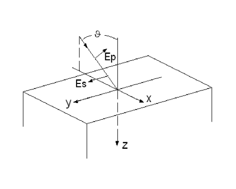
Figure 1: Choice of the coordinate system for the incoming wave. The angle of incidence is given by $\vartheta$. The electric fields in the $p$ polarized wave $E_{p}$ and $s$ polarized wave $E_{s}$ are shown.

Following Kliever and Fuchs KF1 we consider a plane wave of angular frequency $\omega$ incident from vacuum at an angle $\vartheta$ upon the surface of metallic half-space. The geometry, together with the choice of the coordinate system, is shown in Fig. 1. One can separate two polarization states for the wave. For the $s$ polarized wave the electric field is directed in the $y$ axis, while for the $p$ polarized wave the electric field is in the $x-z$ plane and has nonzero $z$ component. For clarity let us sketch out how the specific expressions for the surface impedances have been deduced in Ref. KF1 .

For the $s$ polarized wave the field can be written in the form ${\bf E}=E_{y}(z)\exp(-i\omega t+ik_{x}x)\textbf{n}_{y}$, where $\textbf{n}_{y}$ is the unit vector along the $y$ axis and $k_{x}=\left(\omega/c\right)\sin\vartheta$ is the $x$-component of the wave vector in the incoming wave. Since this component will play significant role in what follows, we will use for it also a special notation $q\equiv k_{x}$, which is settled in the field of the Casimir force. The $z$ dependence of the electric field ${\bf E}=(0,E_{y},0)$ for the $s$ wave inside of metal can be described with the Maxwell equation

$$\frac{d^{2}E_{y}}{dz^{2}}-k_{x}^{2}E_{y}+\frac{\omega^{2}}{c^{2}}D_{y}=0,$$ (3)

where ${\bf D}$ is the displacement field. This equation is valid for $z>0$. Taking the Fourier transform of Eq. (3) over the $z$ coordinate, we obtain

$$-(k_{x}^{2}+k_{z}^{2}){\cal E}_{y}+\frac{\omega^{2}}{c^{2}}{\cal D}_{y}=\frac{dE_{y}\left(+0\right)}{dz}-\frac{dE_{y}\left(-0\right)}{dz},$$ (4)

where ${\cal E}$ and ${\cal D}$ are the Fourier transformed fields defined as

$${\cal E}(k_{z})=\int\limits_{-\infty}^{\infty}dzE\left(z\right)e^{-ik_{z}z}$$ (5)

and similarly for ${\cal D}$. Equation (4) describes the behavior of the electric field in an infinitely extended medium. Furthermore, the right hand side in Eq. (4) is undefined until we find a relation between the two derivatives at the surface. This relation involves describing or modelling the surface. In this work we assume that the electrons scatter elastically from the surface (specular reflection). This assumption is equivalent to assuming an infinitely extended medium, needed to obtain Eq. (4), since an electron bouncing from the surface cannot be distinguished from an electron coming from a fictitious medium on the vacuum side. This is taken into account imposing the symmetry requirements

$$E_{y}\left(z\right)=E_{y}\left(-z\right),\quad D_{y}\left(z\right)=D_{y}\left(-z\right).$$ (6)

Thus, using the Maxwell equation

$$\frac{dE_{y}(+0)}{dz}-\frac{dE_{y}(-0)}{dz}=-i\left(\omega/c\right)H_{x},$$ (7)

and from Eq. (4) one finds

$$\frac{{\cal E}_{y}}{H_{x}\left(+0\right)}=-\frac{2i\omega}{c}\frac{1}{\left(\omega^{2}/c^{2}\right)\varepsilon_{t}-k^{2}},\quad k^{2}=k_{x}^{2}+k_{z}^{2}.$$ (8)

The inverse Fourier transform of this equation evaluated at $z=0$ gives the surface impedance for $s$ polarization:

$$Z_{s}\left(k_{x},\omega\right)\equiv-\frac{E_{y}\left(+0\right)}{H_{x}\left(+0\right)}=\frac{i}{\pi}\frac{\omega}{c}\int\limits_{-\infty}^{\infty}\frac{dk_{z}}{\left(\omega^{2}/c^{2}\right)\varepsilon_{t}-k^{2}}.$$ (9)

For $p$ polarization the problem is slightly more complicated since we have two non-vanishing components of the electric field $E_{x}$ and $E_{z}$. Following a similar line of reasonings as before, the impedance for $p$ polarization is obtained as:

$$Z_{p}\left(k_{x},\omega\right)\equiv\frac{E_{x}\left(+0\right)}{H_{y}\left(+0\right)}=\frac{i}{\pi}\frac{\omega}{c}\int\limits_{-\infty}^{\infty}\frac{dk_{z}}{k^{2}}\left[\frac{k_{x}^{2}}{\left(\omega^{2}/c^{2}\right)\varepsilon_{l}}+\frac{k_{z}^{2}}{\left(\omega^{2}/c^{2}\right)\varepsilon_{t}-k^{2}}\right].$$ (10)

It is natural that both the longitudinal $\varepsilon_{l}\left({\bf k},\omega\right)$ and transverse $\varepsilon_{t}\left({\bf k},\omega\right)$ dielectric functions contribute to $Z_{p}$ because in the $p$ wave the electric field has both components.

Since the impedance approach caused recently some confusion in the field of the Casimir force BKR ; SL4 ; GKM , a few comments concerning the impedances Eq. (9) and Eq. (10) should be made. First, there is not one but two impedances corresponding two different polarizations. Second, the impedances depend not only on the frequency but also on the wave vector along the metal surface $q=k_{x}=\left(\omega/c\right)\sin\vartheta$. Only for the normal incidence the impedances for $p$ and $s$ polarized waves coincide and depend only on frequency. Third, no specific assumptions about the dielectric functions $\varepsilon_{l}$ and $\varepsilon_{t}$ were made in the derivation of Eq. (9) and Eq. (10). In particular, the local functions $\varepsilon_{l}\left(0,\omega\right)=\varepsilon_{t}\left(0,\omega\right)=\varepsilon\left(\omega\right)$ can be used. In this case the integrals can be easily calculated to find so called classical or local impedances

$$Z_{s}^{loc}\left(q,\omega\right)=\frac{1}{\sqrt{\varepsilon\left(\omega\right)-\left(cq/\omega\right)^{2}}},\quad Z_{p}^{loc}\left(q,\omega\right)=\frac{\sqrt{\varepsilon\left(\omega\right)-\left(cq/\omega\right)^{2}}}{\varepsilon\left(\omega\right)}.$$ (11)

These expressions completely coincide with those introduced in Refs. MVE ; EVM and, as was shown there, exactly reproduce the Casimir force in the dielectric function approach. The Leontovich impedance used in Refs. BKR ; SL4 ; GKM from the beginning was introduced as the approximate one LP10 ; Abr for applications in radiophysics. For the propagating waves it really has sense because $cq/\omega\leq 1$ but for metals in the microwave range $\left|\varepsilon\left(\omega\right)\right|\gg 1$. So one can neglect the wave vector along the plates ($q=k_{x}$) in the impedances to get just one frequency dependent function. However, in the Casimir force significant contribution comes from the evanescent fields for which $cq/\omega>1$. In this case the Leotovich approximation fails especially in the limit $\omega\rightarrow 0$, which is important for the analysis of the temperature correction.

The dielectric functions were found KF1 solving the Boltzmann equation and the result is the following

$$\varepsilon_{t}\left(k,\omega\right)=1+\chi_{IB}\left(\omega\right)-\frac{\omega_{p}^{2}}{\omega\left(\omega+i\omega_{\tau}\right)}f_{t}\left(u\right),$$ (12)

$$\varepsilon_{l}\left(k,\omega\right)=1+\chi_{IB}\left(\omega\right)-\frac{\omega_{p}^{2}}{\omega\left(\omega+i\omega_{\tau}\right)}f_{l}\left(u\right),$$ (13)

where the phenomenological susceptibility $\chi_{IB}\left(\omega\right)$ was introduced to describe the interband transitions since these processes are beyond the quasi-free electron model. The functions $f_{t,l}\left(u\right)$ taking into account nonlocal effects are defined in the following way

$$f_{t}\left(u\right)=\frac{3}{2u^{3}}\left[u-\frac{1}{2}\left(1-u^{2}\right)\ln\left(\frac{1+u}{1-u}\right)\right],$$ (14)

$$f_{l}\left(u\right)=\frac{3}{u^{3}}\left[-u+\frac{1}{2}\ln\left(\frac{1+u}{1-u}\right)\right]\cdot\left[1+i\frac{\omega_{\tau}}{\omega}-\frac{i}{2u}\frac{\omega_{\tau}}{\omega}\ln\left(\frac{1+u}{1-u}\right)\right]^{-1},$$ (15)

where the variable $u$ responsible for the nonlocal effects is

$$\qquad u=\frac{v_{F}k}{\omega+i\omega_{\tau}},$$ (16)

and $v_{F}$ is the Fermi velocity. In the local limit $k\rightarrow 0$ both functions (12) and (13) reduce to the local dielectric function (Drude plus interband transitions)

$$\varepsilon\left(\omega\right)=1+\chi_{IB}\left(\omega\right)-\frac{\omega_{p}^{2}}{\omega\left(\omega+i\omega_{\tau}\right)}.$$ (17)

The function $\varepsilon_{t}$ was found first by Reuter and Sondheimer RS . Since these authors considered only the normal incidence, in their work there was no $\varepsilon_{l}$. This function appears at non-normal incidence. In the $p$ wave there is the normal field component $E_{z}$ giving rise to charge fluctuations to which the system responds via the longitudinal dielectric function. It should be mentioned that with the charge fluctuations the relaxation of the perturbed electron distribution toward equilibrium was chosen to the local state of charge imbalance but not to the uniform distribution. The denominator in Eq. (15) describes this effect.

The equations (12)-(16) are used in the optics of metals Book2 to predict the reflectance or absorptance of the materials. It is easy to find the reflection amplitudes $r_{s}$ and $r_{p}$ for $s$ and $p$ polarizations expressed via the impedances as:

$$r_{s}=\frac{\frac{\omega}{c}-Z_{s}\sqrt{\frac{\omega^{2}}{c^{2}}-q^{2}}}{\frac{\omega}{c}+Z_{s}\sqrt{\frac{\omega^{2}}{c^{2}}-q^{2}}},\quad r_{p}=\frac{\sqrt{\frac{\omega^{2}}{c^{2}}-q^{2}}-\frac{\omega}{c}Z_{p}}{\sqrt{\frac{\omega^{2}}{c^{2}}-q^{2}}+\frac{\omega}{c}Z_{p}}.$$ (18)

The reflectance and absorptance are given by:

$$R_{s,p}=\left|r_{s,p}\right|^{2},\quad A_{s,p}=1-\left|r_{s,p}\right|^{2}.$$ (19)

In what follows we will use dimensionless variables, which are more convenient for numerical calculations. We define

$$\Omega=\frac{\omega}{\omega_{p}},\quad Q=\frac{cq}{\omega_{p}},\quad\gamma=\frac{\omega_{\tau}}{\omega_{p}}.$$ (20)

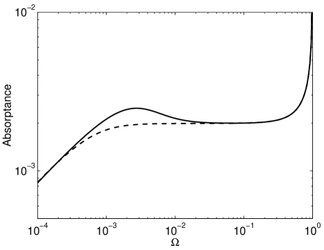
Figure 2: Absorptance as a function of the dimensionless frequency $\Omega$ at normal incidence $\vartheta=0$. Local and nonlocal cases are represented by the dashed and solid lines, respectively. At $\vartheta=0$ there is no difference between $s$ and $p$ polarizations. Parameters were chosen as in Ref. KF1 : $\gamma=1\cdot 10^{-3}$, $v_{F}=0.85\cdot 10^{8}\ cm/s$.

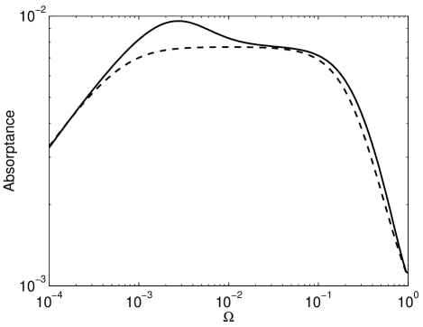
Figure 3: Absorptance as a function of $\Omega$ for $p$ polarization at the incidence angle $\vartheta=75^{\circ}$. Local and nonlocal cases are represented by the dashed and solid lines, respectively. Parameters were chosen as in Fig. 2.

To verify the procedure we recalculated the absorptance with $\gamma=10^{-3}$ and the Fermi velocity $v_{F}=0.85\cdot 10^{8}\;cm/s$ (potassium) to compare with the same calculations in Ref. KF1 . The results are presented in Figs. 2 and 3. Absorptance at the normal incidence $\vartheta=0$ ($Q=0$) is shown in Fig 2. In this case both polarizations give the same result. The nonlocal case is presented by the solid line. The absorptance in the local limit calculated with the impedances (11) is given by the dashed line. The usual increase in the absorptance can be seen at low frequencies $\Omega\sim 10^{-3}$ due to the anomalous skin effect. For the incidence angle $\vartheta=75^{\circ}$ the absorptance of the $p$ polarized wave is shown in Fig. 3. In this case there is an additional peak in absorptance at higher frequencies $\Omega\sim 0.1$. It appears only for $p$ polarization; the $s$ polarization behaves similar to the case $\vartheta=0$. At smaller $\gamma$ both of the peaks become much more significant. These results are in full agreement with those of Kliewer and Fuchs KF3 .

II.2 Evanescent fields

The fluctuating currents in the plates are the sources of fluctuating electromagnetic fields responsible for the Casimir force. The typical separation between bodies in the Casimir force experiments is smaller than the wavelength $\lambda$ of visible light. If we consider one plate as an emitter and the other one as a receiver, then for significant part of the spectrum contributing in the force the receiver will be in the near field zone of the emitter. In this case the propagating field radiated by the emitter will be small in comparison with the evanescent field which exists around the emitter at the distances $\sim\lambda$. The well known example of such an emitter is the Hertz dipole. At small distances from the dipole $\omega r/c\ll 1$ one can neglect the retardation and the field around the source is just the field of the static dipole decaying as $1/r^{2}$. When the force is calculated using the Green function method LP9 , the Green function is exactly the dipole field modified by the presence of the plates. The planar geometry of the problem makes it preferable to expand the dipole field on the plane waves. The plane waves obeying the condition $\omega^{2}/c^{2}<q^{2}$ do not propagate in the gap because the normal component of the wave vector is pure imaginary.

There were some speculations in the literature (see, for example, GKM ), inspired by the problem with the temperature correction to the Casimir force, that for the evanescent fields, the standard expressions for the Fresnel reflection coefficients should be modified. In this connection we have to stress that the evanescent fields are the subject of the near-field optics Cour (see also WJ for a review), where standard electrodynamic approaches are used. Additionally, the longitudinal dielectric function can be probed in the evanescent range by the scattering of a beam of charged particles or fast electrons from the material Book3 . In this way the function $Im\{1/\varepsilon_{l}({\bf k},\omega)\}$ can be directly extracted from the experiment, where ${\bf k}$ is connected with the momentum and $\omega$ with the energy losses of the charged particles. No necessity for modification of the standard electrodynamics was noted so far. A consistent way for the description of evanescent fields is just the analytic continuation of the Eqs. (9), (10), (12)-(16), and Eq. (18) to the range $\omega^{2}/c^{2}<q^{2}$.

Originally the Lifshitz formula for the Casimir force was written as an integral over real frequencies $\omega$ Lif . In this representation one has to calculate first the integral over the variable $p=\sqrt{1-(cq/\omega)^{2}}$ in the range $0<p<1$ (propagating fields) and then integrate over the imaginary axis $p=i\left|p\right|$ from zero to infinity (evanescent fields). So the propagating and evanescent fields were clearly separated. The alternative representation of the same formula LP9 is more popular because of faster convergence of the integrals. In this case the integration is done over the imaginary frequencies $\omega=i\zeta$ but the inner integral over $p=\sqrt{1+(cq/\zeta)^{2}}$ is calculated from $1$ to $\infty$. Formally we are always in the evanescent domain because at imaginary frequencies the normal component of the wave vector is pure imaginary $k_{z}=i\sqrt{\zeta^{2}/c^{2}+q^{2}}$.  For this reason we will not investigate specially the domain $q^{2}>\omega^{2}/c^{2}$ making the analytic continuation on $q$ but instead we will make the analytic continuation to imaginary frequencies. This procedure is well defined for the response functions which are analytical in the upper half of complex plane $\omega$. In the electrodynamics the response functions are the components of the Green function $\varepsilon_{l}^{-1}\left({\bf k},\omega\right)$ and $\left[\left(\omega^{2}/c^{2}\right)\varepsilon_{t}\left({\bf k},\omega\right)-k^{2}\right]^{-1}$ but not the dielectric functions themselves Mar ; Kir . Exactly these expressions take part in the impedances (9) and (10) and, therefore, the impedances can be considered as analytical functions of $\omega$.

Using the dimensional variables (20) the impedances at imaginary frequencies ($\Omega\rightarrow i\Omega$) can be written as

$$Z_{s}\left(Q,\Omega\right)=\frac{2}{\pi}\frac{\Omega}{Q}\int\limits_{0}^{\infty}\frac{\cosh\chi\,d\chi}{\cosh^{2}\chi+\frac{\Omega^{2}}{Q^{2}}\varepsilon_{t}\left(\Omega,v\right)},$$ (21)

$$Z_{p}\left(Q,\Omega\right)=\frac{2}{\pi}\frac{\Omega}{Q}\int\limits_{0}^{\infty}\frac{d\chi}{\cosh\chi}\left[\frac{1}{\frac{\Omega^{2}}{Q^{2}}\varepsilon_{l}\left(\Omega,v\right)}+\frac{\cosh^{2}\chi\,-1}{\cosh^{2}\chi+\frac{\Omega^{2}}{Q^{2}}\varepsilon_{t}\left(\Omega,v\right)}\right].$$ (22)

Here we introduced a new variable of integration $\chi$ which is defined by the relation $k_{z}=k_{x}\sinh\chi$. For the dielectric functions at imaginary frequencies one finds

$$\varepsilon_{l}\left(\Omega,v\right)=1+\chi_{IB}\left(\Omega\right)+\frac{f_{l}\left(v\right)}{\Omega\left(\Omega+\gamma\right)},\quad f_{l}\left(v\right)=\frac{3}{v^{2}}\frac{v-\arctan v}{v+\frac{\gamma}{\Omega}\left(v-\arctan v\right)},$$ (23)

$$\varepsilon_{t}\left(\Omega,v\right)=1+\chi_{IB}\left(\Omega\right)+\frac{f_{t}\left(v\right)}{\Omega\left(\Omega+\gamma\right)},\quad f_{t}\left(v\right)=\frac{3}{2v^{3}}\left[-v+\left(1+v^{2}\right)\arctan v\right],$$ (24)

$$v=\frac{v_{F}}{c}\frac{Q}{\Omega+\gamma}\cosh\chi.$$ (25)

These formulas are used for numerical calculations of the impedances. They have to be compared with the classical expressions in the local limit which follows from Eq. (11) after the change to imaginary frequencies:

$$Z_{s}^{loc}=\frac{1}{\sqrt{\varepsilon\left(\Omega\right)+\frac{Q^{2}}{\Omega^{2}}}},\quad Z_{p}^{loc}=\frac{\sqrt{\varepsilon\left(\Omega\right)+\frac{Q^{2}}{\Omega^{2}}}}{\varepsilon\left(\Omega\right)},\quad\varepsilon\left(\Omega\right)=1+\chi_{IB}\left(\Omega\right)+\frac{1}{\Omega\left(\Omega+\gamma\right)}.$$ (26)

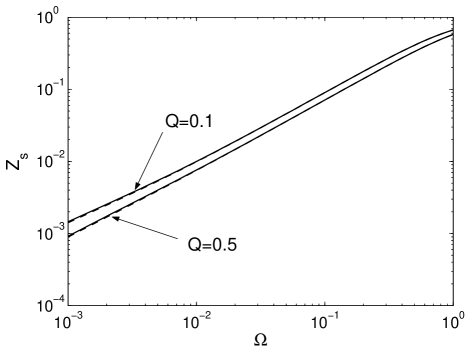
Figure 4: Numerically calculated impedance $Z_{s}$ as a function of dimensionless frequency $\Omega$ for two values of the dimensionless wave numbers along the plate $Q$. Solid line describes nonlocal calculations; the dashed line present the local case. Maximal deviation between local and nonlocal curves is about 2%. Gold parameters were used for calculation: $\gamma=3\cdot 10^{-3}$, $v_{F}=1.4\cdot 10^{8}\ cm/s$.

The numerical result for $Z_{s}$ is shown in Fig. 4 as a function of $\Omega$ for two values of $Q$. All calculations were performed for the parameters corresponding to gold at room temperature: $\gamma=3\cdot 10^{-3}$, $v_{F}=1.4\cdot 10^{8}\;cm/s$, $\omega_{p}=1.37\cdot 10^{16}\;rad/s$. The impedance of the local theory is presented by the dashed lines. One can see that the nonlocal effect is very small for this polarization. The largest deviation from the local curves is just about of 2%. Obviously the $s$ polarization cannot produce significant nonlocal correction to the Casimir force.

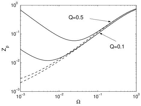
Figure 5: Numerically calculated impedance $Z_{p}$ as a function of frequency $\Omega$ for two values of the wave numbers along the plate $Q$. Nonlocal and local cases are shown by the solid and dashed lines, respectively.

A different situation is realized for $p$ polarization, as shown in Fig. 5. One can see that there is a significant difference between the local and nonlocal cases. The deviation increases with frequency decrease and becomes larger for larger $Q$. This behavior has deep physical meaning, as explained below, and can appear only for the evanescent fields. Since in both cases the deviations from the local case are in the low frequency range, we analyze this limit analytically.

II.3 Low frequency behavior of impedances

At low frequencies $\Omega\lesssim\gamma$, the variable $v$ defined by Eq. (25) can be large if $\gamma\lesssim v_{F}/c\approx 4.7\cdot 10^{-3}$. Let us consider the impedances in the limit $v\gg 1$. In this limit the functions $f_{l}\left(v\right)$ and $f_{t}\left(v\right)$ in Eq. (23 ) and Eq. (24) behave as

$$f_{l}\left(v\right)\approx\frac{3}{v^{2}}\frac{\Omega}{\Omega+\gamma},\quad f_{t}\left(v\right)\approx\frac{3\pi}{4v},\quad v\gg 1.$$ (27)

In the transverse dielectric function $\varepsilon_{t}$ one can neglect $1+\chi_{IB}\left(\Omega\right)$ since the third term behaves as $1/\Omega$ at low frequencies. It gives for $\varepsilon_{t}\left(\Omega,v\right)$

$$\varepsilon_{t}\left(\Omega,v\right)\approx\frac{4\pi}{3}\frac{c}{v_{F}}\frac{1}{Q\cosh\chi}\frac{1}{\Omega}.$$ (28)

For the the longitudinal function $\varepsilon_{l}$ the phenomenological susceptibility $\chi_{IB}\left(\Omega\right)$ again is negligible because it is responsible for the interband transitions at much higher frequencies but we cannot neglect the unit since the third term in (23) does not depend on frequency at all and not necessarily large. For $\varepsilon_{l}\left(\Omega,v\right)$ one find

$$\varepsilon_{l}\left(\Omega,v\right)\approx 1+3\left(\frac{c}{v_{F}}\frac{1}{Q\cosh\chi}\right)^{2}=1+3\left(\frac{\omega_{p}}{v_{F}}\frac{1}{k}\right)^{2}.$$ (29)

This expression describes the Thomas-Fermi screening of the longitudinal electric field. It has to be true KF2 at $\Omega<\gamma$ and $k$ much smaller than the Fermi wave number $k_{F}$ that is the applicability range of the Thomas-Fermi approximation. The latter condition $k\ll k_{F}$ is also the condition for applicability of the Boltzmann equation.

Substituting (28) and (29) in Eqs. (21) and (22) one finds for the impedances

$$Z_{s}=\frac{\Omega}{Q}F(b),$$ (30)

$$Z_{p}=\frac{Q}{\Omega}\frac{1}{\sqrt{1+3\left(c/v_{F}Q\right)^{2}}}+\frac{\Omega}{Q}G(b)\approx\frac{1}{\sqrt{3}}\frac{Q^{2}}{\Omega}\frac{v_{F}}{c}+\frac{\Omega}{Q}G(b),$$ (31)

where the functions $F\left(b\right)$ and $G\left(b\right)$ are defined as

$$F(b)=\frac{2}{\pi}\int\limits_{0}^{\infty}d\chi\frac{\cosh^{2}\chi}{\cosh^{3}\chi+b^{3}},\quad G\left(b\right)=\frac{2}{\pi}\int\limits_{0}^{\infty}d\chi\frac{\sinh^{2}\chi}{\cosh^{3}\chi+b^{3}},$$ (32)

$$b=\frac{1}{Q}\left(\frac{3\pi}{4}\frac{c}{v_{F}}\Omega\right)^{1/3}.$$ (33)

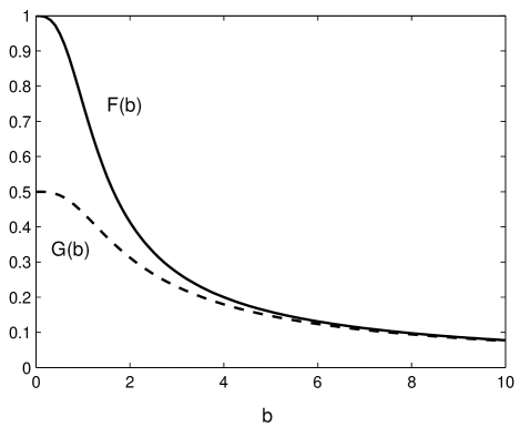
Figure 6: Numerically calculated functions $F(b)$ and $G(b)$.

The functions $F(b)$ and $G(b)$ can be found explicitly but the result is cumbersome and inconvenient for analysis. For this reason we calculated the integrals in Eq. (32) numerically presenting explicitly only the asymptotics at $b\ll 1$ and $b\gg 1$. The functions $F(b)$ and $G(b)$ are shown in Fig. 6. The asymptotic behavior of these functions is

$$F(b)=\left\{\begin{array}[]{c}1-\frac{4}{3\pi}b^{3},\quad b\ll 1\\ \frac{4}{3\sqrt{3}}\frac{1}{b}+\frac{1}{\pi b^{3}}\left(\ln 2b-1/2\right),\quad b\gg 1\end{array}\right.$$

$$G(b)=\left\{\begin{array}[]{c}\frac{1}{2}-\frac{4}{15\pi}b^{3},\quad b\ll 1\\ \frac{4}{3\sqrt{3}}\frac{1}{b}-\frac{1}{\pi b^{3}}\left(\ln 2b+1/2\right),\quad b\gg 1\end{array}\right.$$ (34)

The known result for the Leontovich impedance for the strong anomalous skin effect RS ; LP10 ; Abr is easily reproduced if we take in the equations above the limit $Q\rightarrow 0$. In this limit the parameter $b$ goes to infinity and the contribution of the transverse dielectric function is the same for both polarization: $F(b)=G(b)=4/3\sqrt{3}b$. The contribution from $\varepsilon_{l}$ in $Z_{p}$ disappears in the limit $Q\rightarrow 0$. Hence, the impedances will coincide with each other and they are given by the classical expression for the strong anomalous skin effect continued to imaginary frequencies

$$Z_{s}(0,\Omega)=Z_{p}\left(0,\Omega\right)=Z\left(\Omega\right)=\frac{4}{3\sqrt{3}}\left(\frac{4}{3\pi}\frac{v_{F}}{c}\Omega^{2}\right)^{1/3}.$$ (35)

However, if $Q$ is nonzero there is a small enough frequency where $b$ is not large anymore and Eq. (35) is not applicable. When $\Omega$ is so small that $b\ll 1$ the impedance $Z_{s}$ approaches the limit $\Omega/Q$. The same limit is realized for the local impedance $Z_{s}^{loc}$ in Eq. (26) at very low frequencies when one can neglect $\varepsilon\left(\Omega\right)$ in comparison with $Q^{2}/\Omega^{2}$.

For $p$ polarization at nonzero $Q$ the contribution of $\varepsilon_{t}$ in the impedance decreases with $\Omega$ but the contribution of $\varepsilon_{l}$ increases as $1/\Omega$ (see Eq. (31)) and dominates in $Z_{p}$ at low frequencies. It is in agreement with our numerical calculations in Fig. 5. Indeed this is the result of the Thomas-Fermi screening. The same effect is not realized for the propagating fields. In this case the ratio $Q/\Omega=\sin\vartheta\leq 1$ is restricted. Since $v_{F}/c=4.7\cdot 10^{-3}$ is small, the variable $u$ (16) is small nearly everywhere in the integration range and the function $f_{l}\left(u\right)\approx 1$. Therefore the local limit is realized instead for the longitudinal contribution in $Z_{p}$.

The behavior of the impedance for the $s$ polarization at low frequencies is a sensitive matter for the temperature correction to the Casimir force. One of us (VBS) in collaboration with M. Lokhanin analyzed this problem SL4 with the Leontovich impedance (35). As follows from the discussion above this analysis has to be reconsidered taking into account not only different behavior of $Z_{s}$ at very low frequencies but also significant deviation of $Z_{p}$ from the local impedance in this range.

III Nonlocal correction to the Casimir force

In this section we are going to estimate the correction to the Casimir force due to nonlocal effects at frequencies smaller than $\omega_{p}$. The restriction on frequency is connected with the use of the Boltzmann approximation for the dielectric functions (23), (24). In this approximation we cannot describe the plasmon excitations. Of course, one could use more general dielectric functions like those in the self-consistent-field approximation KF2 to analyze all the nonlocal effects. However, we think it is reasonable to separate the effects of different physical origin. Influence of the plasmon excitations on the Casimir force has been already evaluated EVM using the hydrodynamic approximation for the longitudinal dielectric function, but the correction to the force due to the anomalous skin effect never has been calculated before. Only specific questions concerning the temperature correction have been addressed in the literature SL4 . By anomalous skin effect we refer not only to the strong anomalous skin effect that is realized when the electron mean free path is larger than the field penetration depth, but to all the nonlocal effects that happen at frequencies smaller than $\omega_{p}$.

We will consider only the force in the zero temperature limit. Thus, the Casimir force will be calculated without the temperature correction but all the other parameters characterizing the material, especially the relaxation frequency $\omega_{\tau}$, will be kept at finite temperature. The results of the previous section for the impedances $Z_{s}$ and $Z_{p}$ are important for the temperature correction problem but this question will be considered elsewhere.

It is known that when a metal is described by the surface impedances, the Lifshitz formula for the Casimir force LP9 remains essentially the same MT ; EVM as when the metal is described by the local dielectric function. Only the reflection coefficients have to be expressed via the impedances. At nonzero temperature the Lifshitz formula includes summation over the Matsubara frequencies $\zeta_{n}$, defined for our dimensionless frequency as

$$\Omega_{n}=\frac{\zeta_{n}}{\omega_{p}}=\frac{2\pi nkT}{\hbar\omega_{p}}.$$ (36)

To get the Casimir force at $T=0$ we have to integrate over the continuous variable $\Omega$. In the dimensionless variables $\Omega$ and $Q$ the Casimir force between two metallic plates separated by the distance $a$ at $T=0$ is

$$F_{pp}\left(a\right)=-\frac{\hbar c}{2\pi^{2}\delta^{4}}\int\limits_{0}^{\infty}d\Omega\int\limits_{0}^{\infty}dQQ\sqrt{\Omega^{2}+Q^{2}}\left[\left(r_{s}^{-2}\exp\left(2d\sqrt{\Omega^{2}+Q^{2}}\right)-1\right)^{-1}+\right.$$

$$\left.\left(r_{p}^{-2}\exp\left(2d\sqrt{\Omega^{2}+Q^{2}}\right)-1\right)^{-1}\right],$$ (37)

where

$$d=\frac{a}{\delta},\quad\delta=\frac{c}{\omega_{p}}\approx 21.88\;nm.$$ (38)

Here $\delta$ is the penetration depth for gold. The reflection coefficients follows from Eq. (18) after continuation to imaginary frequencies

$$r_{s}=\frac{\Omega-\sqrt{\Omega^{2}+Q^{2}}Z_{s}\left(\Omega,Q\right)}{\Omega+\sqrt{\Omega^{2}+Q^{2}}Z_{s}\left(\Omega,Q\right)},\quad r_{p}=\frac{\sqrt{\Omega^{2}+Q^{2}}-\Omega Z_{p}\left(\Omega,Q\right)}{\sqrt{\Omega^{2}+Q^{2}}+\Omega Z_{p}\left(\Omega,Q\right)}.$$ (39)

The impedances $Z_{s,p}$ are calculated according to Eqs. (21)-(25).

The force between a sphere and a plane can be calculated with the help of the proximity force approximation DA which gives the following expression

$$F_{sp}\left(a\right)=\frac{\hbar cR}{2\pi\delta^{3}}\int\limits_{0}^{\infty}d\Omega\int\limits_{0}^{\infty}dQQ\left[\ln\left(1-r_{s}^{2}\exp\left(-2d\sqrt{\Omega^{2}+Q^{2}}\right)\right)+\right.$$

$$\left.\ln\left(1-r_{p}^{2}\exp\left(-2d\sqrt{\Omega^{2}+Q^{2}}\right)\right)\right],$$ (40)

where $R$ is the radius of the sphere.

III.1 Numerical procedure

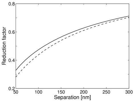
Figure 7: The reduction factor $F_{pp}(a)/F_{c}(a)$ in the local case as a function of the separation $a$ calculated with the handbook data (solid line) and with the Drude model for the dielectric function (dashed line).

First we calculate the force between parallel plates $F_{pp}^{Drude}(a)$ in the local limit with the Drude dielectric function and local impedances (26). The actual calculations were performed for the dimensionless relaxation frequency (see (20)) $\gamma=4\cdot 10^{-3}$. This value is the best fit LR of the handbook optical data for gold HB1 at low frequencies. In Fig. 7 we show the reduction factor $\eta(a)$ defined as the ratio of the calculated force to the original Casimir force (1); this is

$$\eta(a)=\frac{F_{pp}(a)}{F_{c}(a)}.$$ (41)

The force calculated using the Drude model (dashed line) is smaller than that calculated using the handbook optical data for gold (solid line). The solid line coincides with the reduction factor given in Ref. LR .

The nonlocal correction is calculated without the empirical susceptibility $\chi_{IB}\left(\omega\right)$ introduced in Eqs. (12) and (13) so we have to remember that the relative nonlocal correction will be smaller than the calculated one on the value of the order of the relative difference between the curves in Fig. 7 (8% at $a=100$ nm).

The force calculation in the nonlocal case is quite complicated because one has to make three integrations with high precision, one to calculate the impedances and two to calculate the force. It is much more easy to calculate not the force itself but integrate the difference between nonlocal and local integrands. In this case there is no need to perform high precision calculation of the integrals since we have to know the correction due to nonlocality with the precision of about of 10%. Actual calculation of the difference

$$\delta F_{pp}\left(a\right)=F_{pp}^{nonloc}\left(a\right)-F_{pp}^{loc}(a)$$ (42)

were made with the relative accuracy of 1%, while the impedances (21), (22) were calculated with the relative precision of $10^{-6}$. The integrands for $s$ and $p$ polarizations defined as

$$\delta f_{s,p}=Q\sqrt{\Omega^{2}+Q^{2}}\left[\left(r_{s,p}^{-2}\exp\left(2d\sqrt{\Omega^{2}+Q^{2}}\right)-1\right)^{-1}-(r_{s,p}\rightarrow r_{s,p}^{loc})\right]$$ (43)

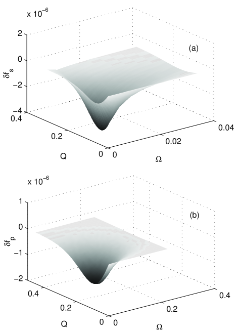
Figure 8: Integrands for $s$ polarization (a) and for $p$ polarization (b). Note different scales in $\Omega$ axes.

are presented for $a=275\;nm$ in Fig. 8(a) and Fig. 8(b), respectively. Both of them are negative as it should be, since the force decreases due to the nonlocal effects. It is interesting to notice that $\delta f_{s}$ is nonzero in a very narrow range of small $\Omega$. In contrast, the integrand for $p$ polarization $\delta f_{p}$ is nonzero in a broader range of $\Omega$ (pay attention on different scales in figures (a) and (b)). Nonlocal effects are always significant in a wider range of $Q\lesssim 1$. With the decrease of separation $a$ the integrand for $p$ polarization increases in the magnitude and becomes wider in both directions $\Omega$ and $Q$. The integrand for $s$ polarization decreases in magnitude and widens only in $Q$ direction. Thus, the contribution of $s$ polarization in the force correction is always smaller than that for the $p$ polarization.

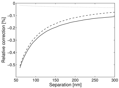
Figure 9: The relative correction to the force due to nonlocal effects for the plate-plate geometry. The solid line presents the resulting correction. The dashed line gives the contribution of the $p$ polarization and the dotted line gives the contribution of the $s$ polarization. Gold parameters were used for calculations.

The results for the relative correction $\delta F_{pp}\left(a\right)/F_{pp}^{Drude}\left(a\right)$ due to the nonlocal effects are presented in Fig. 9. The solid line gives the resulting correction, while the dashed and the dotted lines represent the contributions of $p$ and $s$ polarizations, respectively. One can see that the correction is small but not negligible. Contribution of $s$ polarization increases when $\gamma$ becomes smaller, but even for $\gamma=10^{-5}$ this contribution is still on the level of 0.2%. We can see that large deviation of the impedance for $p$ polarization from the local one that happens at low frequencies is not very significant for the force. This is because in the reflection coefficient $r_{p}$ the impedance enter as $\Omega Z_{p}$ so that $1/\Omega$ behavior of $Z_{p}$ is suppressed in the reflection coefficient.

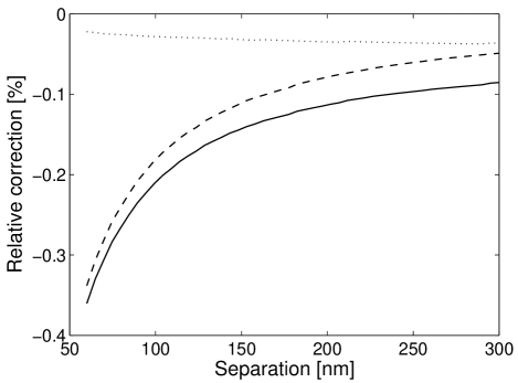
Figure 10: Same as Fig. 9 but for the sphere-plate geometry.

Similar calculations were made for the sphere-plate geometry. The relative correction $\delta F_{sp}\left(a\right)/F_{sp}^{Drude}\left(a\right)$ together with the separate contributions of $p$ and $s$ polarizations is shown in Fig. 10. The behavior of the curves is quite similar to that for the plate-plate geometry. Only the absolute magnitude of the correction is smaller.

IV Discussion

The theory described in Sec. II provides a solid ground for the impedance approach in the Casimir force calculation. Specifically it allows correctly to take into account nonlocal connection between the displacement and electric fields. In this paper we restricted ourselves by the nonlocal effects happening at frequencies smaller than $\omega_{p}$. This restriction is due to used Boltzmann approximation for the nonlocal dielectric functions (12)-(16). However the equations for the impedances (9), (10) are much more general. For specular electron reflection off the surface these equations are true for arbitrary dielectric functions $\varepsilon_{t}\left({\bf k},\omega\right)$ and $\varepsilon_{l}\left({\bf k},\omega\right)$ with the only condition that these functions exist. Therefore, all nonlocal effects can be described on the same basis. In particular, for metals the most general dielectric functions for a free-electron gas were found in the self-consistent-field (or Lindhard) approximation with the necessary modifications to include a finite relaxation time KF2 . In this approximation $\varepsilon_{t}\left(k,\omega\right)$ has the following form

$$\varepsilon_{t}\left(k,\omega\right)=1-\frac{\omega_{p}^{2}}{\omega\left(\omega+i\omega_{\tau}\right)}f_{t}\left(u,z\right),$$

where

$$f_{t}(u,z)=\frac{3}{8}\left(z^{2}+3u^{-2}+1\right)-\frac{3}{32z}\left\{\left[1-\left(z-u^{-1}\right)^{2}\right]^{2}\ln\left(\frac{z-u^{-1}+1}{z-u^{-1}-1}\right)+\right.$$

$$\left.\left[1-\left(z+u^{-1}\right)^{2}\right]^{2}\ln\left(\frac{z+u^{-1}+1}{z+u^{-1}-1}\right)\right\}.$$ (44)

Here $u$ defined as before by Eq. (16) and $z$ is $z=k/2k_{F}$. The longitudinal dielectric function has a little bit more complicated form:

$$\varepsilon_{l}\left(k,\omega\right)=1+(\varepsilon_{w}-1)\left[1+i\frac{\omega_{\tau}}{\omega}-\frac{i}{2u}\frac{\omega_{\tau}}{\omega}\ln\left(\frac{1+u}{1-u}\right)\right]^{-1},$$

$$\varepsilon_{w}=1+\frac{3\omega_{p}^{2}}{k^{2}v_{F}^{2}}f_{l}\left(u,z\right),$$

$$f_{l}\left(u,z\right)=\frac{1}{2}+\frac{1}{8z}\left\{\left[1-\left(z-u^{-1}\right)^{2}\right]\ln\left(\frac{z-u^{-1}+1}{z-u^{-1}-1}\right)+\right.$$

$$\left.\left[1-\left(z+u^{-1}\right)^{2}\right]\ln\left(\frac{z+u^{-1}+1}{z+u^{-1}-1}\right)\right\}.$$ (45)

All the other approximations for the free-electron gas can be found from (44), (45) in definite limit cases. For example, the Boltzmann approximation (12)-(16) follows from (44), (45) in the limit $z\rightarrow 0$. These expressions for the dielectric functions allow to perform detailed investigation of the high frequency region $\omega\gtrsim\omega_{p}$ which gives more significant contribution in the Casimir force due to excitation of the propagating charge density waves in the metal EVM .

We considered here only specular electron reflection off the metal surface. It is justified for the AFM experiment Moh2 where the root mean square (rms) roughness of the surface ($1\;nm$) was much smaller than the mean free path ($30\;nm$). However, in the MEMS experiments Chan ; Decca1 ; Decca2 the rms roughness was comparable with the mean free path and approximation of specular reflection fails. In this case the diffuse reflection of electrons off the surface is more suitable. For the diffuse reflection the impedances are not represented by the Eqs. (9 ), (10) anymore. Instead one has to use the impedances for the diffuse reflection KF3 . There is no problem with $Z_{s}$ which is expressed via $\varepsilon_{t}\left(k,\omega\right)$ but situation with $Z_{p}$ is much more complicated. This occurs because of the destruction of translational invariance in the direction normal to the surface KF3 . Although it is possible to calculate both of the impedances in the diffuse case, we do not think it is reasonable to do for the anomalous skin effect. This is because the nonlocal correction is smaller than the uncertainty in the Casimir force due to the roughness. The roughness correction to the force is usually evaluated using the proximity force approximation (see, for example, Decca2 ). Recently it has been pointed out GLNR that this approach is valid only for long wavelength deformations of the plates. The real surfaces of deposited gold films always roughed on very different scales OASA and the short wavelengths will bring uncertainty in the estimate of the force.

The impedances (9), (10) with the nonlocal dielectric functions (12)-(16) are well known in the optics of metals but in this paper we considered them in the near field range where the nonlocal effects were unexplored. In this sense the Casimir force is a unique problem. Significant contribution in the force comes from fluctuating fields in the near field region. Since the force has to be predicted with high precision, it is important to take into account the nonlocal effects. Though we have found here that the anomalous skin effect gave observable but minor correction to the force, the other nonlocal effects, such as plasmon excitation, can give more significant correction. This paper just provide a regular basis for the calculations of this kind.

V Conclusions

A complete calculation of the Casimir force that can be accurately compared with experiments requires a full optical characterization of the involved materials. This is complicated due to the various factors that can modify the optical properties. In this work we described a systematic way to take into account the nonlocal effects in the material. It was stressed that, in general, a metal had to be described with two different surface impedances corresponding to $s$ and $p$ polarizations and these impedances depend not only on frequency but also on the wave vector along the metal surface. As a specific problem we considered the correction to the Casimir force in the region of the anomalous skin effect ($\omega<\omega_{p}$). This region is characterized by the nonlocal dielectric functions (longitudinal and transverse) that can be obtained in the Boltzman approximation. The impedances are completely defined by these functions.

It was demonstrated that the exact impedances were differed from the approximate Leontovich impedance. The latter one caused confusion in the literature so our analysis resolved the problem and gave a proper description of the impedance approach in the Casimir force calculation. It was emphasized that the significant contribution in the force came from the evanescent fields. For these fields the impedances can be found by the analytic continuation and the procedure is well defined. The contribution of the nonlocal effects in the impedances was found to be quite different for propagating and evanescent fields. Specifically for the evanescent fields the impedance for $p$ polarization deviates significantly from the local one that is the result of the Thomas-Fermi screening. For $s$ polarization the nonlocal contribution in the impedance is more significant for the propagating fields than for the evanescent ones.

In the impedance approach the Casimir force can be found from the same Lifshitz formula in which the reflection coefficients are expressed via the impedances. We calculated the nonlocal correction to the force in the region of anomalous skin effect at zero temperature. In spite of significant deviation of $Z_{p}$ from the local impedance the nonlocal reflection coefficient $r_{p}$ deviates from the local one only slightly. For the $s$ polarization the effect is even smaller. For this reason the total contribution of the nonlocal effects in the Casimir force is on the level of $0.5\%$ at small separations. It is a minor effect within the levels of detectability of present experiments, but smaller than the corrections introduced due to sample roughness.

We did not considered in this paper the temperature correction though it is clear from the analysis of impedances that anomalous skin effect will be important for the temperature correction. A new phenomenon observed here is that the reflection coefficient $r_{p}$ for $p$ polarization is not going to 1 in the zero frequency limit $\omega\rightarrow 0$. This behavior is the result of the Thomas-Fermi screening.

The technic developed in this paper can be applied to calculate the contribution of the other nonlocal effects such as plasmon excitation at $\omega\sim\omega_{p}$. These effects are expected to give more significant correction to the Casimir force.

- (1) H. B. G. Casimir, Proc. K. Ned. Akad. Wet. 51, 793 (1948).
- (2) S. K. Lamoreaux, Phys. Rev. Lett. 78, 5 (1997); 81, 5475 (1998).
- (3) U. Mohideen and A. Roy, Phys. Rev. Lett. 81, 4549 (1998); A. Roy, C.-Y. Lin, and U. Mohideen, Phys. Rev. D 60, 111101(R) (1999).
- (4) B. W. Harris, F. Chen, and U. Mohideen, Phys. Rev. A 62, 052109 (2000).
- (5) T. Ederth, Phys. Rev. A 62, 062104 (2000).
- (6) H. B. Chan, V. A. Aksyuk, R. N. Kleiman, D. J. Bishop, and F. Capasso, Science 291, 1941 (2001); Phys. Rev. Lett. 87, 211801 (2001).
- (7) G. Bressi, G. Carugno, R. Onofrio, and G. Ruoso, Phys. Rev. Lett. 88, 041804 (2002).
- (8) R. S. Decca, D. López, E. Fischbach, and D. E. Krause, Phys. Rev. Lett. 91, 050402 (2003).
- (9) R. S. Decca, E. Fischbach, G. L. Klimchitskaya, D. E. Krause, D. López, and V. M. Mostepanenko , Phys. Rev. D 68, 116003 (2003).
- (10) The precision claimed in some experiments is overestimated due to several sensitive factors such as roughness. Small errors in roughness can give rise to large theoretical corrections as pointed out in D. Iannuzzi, I. Gelfand, M. Lisanti, and F. Capasso, arXiv:quant-ph/0312043 vi (2003).
- (11) E. M. Lifshitz, Zh. Eksp. Teor. Fiz. 29, 94 (1956) [Sov. Phys. JETP 2, 73 (1956)].
- (12) E. M. Lifshitz and L. P. Pitaevskii, Statistical Physics, Part 2 (Pergamon Press, Oxford, 1980).
- (13) Handbook of Optical Constants of Solids, edited by E.D. Palik (Academic Press, 1995).
- (14) V.M. Zolotarev, V.N. Morozov, and E.V. Smirnova, Optical constants of natural and technical media (Khimija, Leningrad, 1984) (in Russian).
- (15) S. K. Lamoreaux, Phys. Rev. A 59, R3149 (1999).
- (16) M. Boström and Bo E. Sernelius, Phys. Rev. A 61 046101 (2000).
- (17) A. Lambrecht and S. Reynaud, Eur. Phys. J. D 8, 309 (2000).
- (18) V. B. Svetovoy and M. V. Lokhanin, Mod. Phys. Lett. A 15, 1437 (2000).
- (19) G. L. Klimchitskaya, U. Mohideen, and V. M. Mostepanenko, Phys. Rev. A 61, 062107 (2000).
- (20) V. B. Svetovoy and M. V. Lokhanin, Mod. Phys. Lett. A 15, 1013 (2000).
- (21) V. Svetovoy, Proc. Quantum Field Theory Under External Conditions 2003, Ed. K. A. Milton (Rynton Press, 2003) (unpublished).
- (22) V. B. Bezerra, G. L. Klimchitskaya, and C. Romero, Phys. Rev. A 65, 012111 (2002).
- (23) V. B. Svetovoy and M. V. Lokhanin, Phys. Rev. A 67, 022113 (2003).
- (24) B. Geyer, G. L. Klimchitskaya, and V. M. Mostepanenko, Phys. Rev. A 67, 062102 (2003).
- (25) V. M. Mostepanenko and N. N. Trunov, Yad. Fiz. 42, 1297 (1985) [Sov. J. Nucl. Phys. 42, 818 (1985)].
- (26) L. D. Landau and E. M. Lifshitz, Electrodynamics of Continuous Media (Pergamon Press, Oxford, 1984).
- (27) M. Boström and Bo E. Sernelius, Phys. Rev. Lett. 84, 4757 (2000); Bo E. Sernelius, ibid. 87, 139102 (2001); Bo E. Sernelius and M. Boström, ibid. 87, 259101 (2001).
- (28) M. Bordag, B. Geyer, G. L. Klimchitskaya, and V. M. Mostepanenko, Phys. Rev. Lett. 85, 503 (2000); ibid. 87, 259102 (2001).
- (29) C. Genet, A. Lambrecht, and S. Reynaud, Phys. Rev. A 62, 012110 (2000).
- (30) S. K. Lamoreaux, Phys. Re. Lett. 87, 139101 (2001).
- (31) V. B. Svetovoy and M. V. Lokhanin, Phys. Lett. A 280, 177 (2001).
- (32) G. L. Klimchitskaya and V. M. Mostepanenko, Phys. Rev. A 63, 062108 (2001).
- (33) I. Brevik, J. B. Aarseth, and J. S. Høye, Phys. Rev. E 66, 026119 (2002).
- (34) J. S. Høye, I. Brevik, J. B. Aarseth, and K. A. Milton, Phys. Rev. E 67, 056116 (2003).
- (35) W. L. Mochán, C. Villarreal, and R. Esquivel-Sirvent, Rev. Mex. Fis. 48, 339 (2002).
- (36) E. M. Lifshitz and L. P. Pitaevskii, Physical Kinetics (Pergamon Press, Oxford, 1981).
- (37) A. A. Abrikosov, Fundamentals of the Theory of Metals (North-Holland, Amsterdam, 1988).
- (38) R. Esquivel, C. Villarreal, and W. L. Mochán, Phys. Rev. A 68, 052103 (2003).
- (39) K. L. Kliewer and R. Fuchs, Phys. Rev. 172, 607 (1968).
- (40) W. E. Jones, K. L. Kliewer, and R. Fuchs, Phys. Rev. 178, 1201 (1969); K. L. Kliewer and R. Fuchs, ibid. 181, 652 (1969); 185, 905 (1969).
- (41) K. L. Kliewer and R. Fuchs, Phys. Rev. B 2, 2923 (1970); J. M. Keller, R. Fuchs, and K. L. Kliewer, ibid. 12, 2012 (1975).
- (42) G. E. H. Reuter and E. H. Sondheimer, Proc. Roy. Soc. A 195, 336 (1948).
- (43) A. B. Pippard, Proc. Roy. Soc. A 191, 385 (1947).
- (44) Y.Y. Wang, F.C. Zhang, V.P. Dravid et al., arXiv-cond-mat: 960606v1; Phys. Rev. Lett. 75, 2546 (1995).
- (45) P. Halevi, Spatial Dispersion in Solids and Plasmas, Electromagnetic Waves Vol. 1, ed. by P. Halevi (North-Holland, Amsterdam, 1992).
- (46) D. Courjon, Near-field Microscopy and Near field Optics (Imperial College Press, 2003).
- (47) E. Wolf and D. F.V. James, Rep. Prog. Phys. 59, 771 (1996).
- (48) M. Dressel and G. Gruner, Electrodynamics of Solids, (Cambridge University Press, 2002).
- (49) P. C. Martin, Phys. Rev., 161, 143 (1967).
- (50) D.A. Kirzhnits in: The Dielectric Function of Condensed Systems, eds., L.V. Keldysh, D.A. Kirzhnits, and A.A. Maradudin, (Elsevier Publ., 1989).
- (51) B. Derjaguin and A. Abrikosova, Sov. Phys. JETP 3, 819 (1957).
- (52) C. Genet, A. Lambrecht, P. Maia Neto, and S. Reynaud, Euro. Phys. Lett. 62, 484 (2003).
- (53) A. I. Oliva, E. Anguiano, J. L. Sacedón, and M. Aguilar, Phys. Rev. B 60, 2720 (1999).