Gaussian quantum Monte Carlo methods for fermions

Abstract

We introduce a new class of quantum Monte Carlo methods, based on a Gaussian quantum operator representation of fermionic states. The methods enable first-principles dynamical or equilibrium calculations in many-body Fermi systems, and, combined with the existing Gaussian representation for bosons, provide a unified method of simulating Bose-Fermi systems. As an application, we calculate finite-temperature properties of the two dimensional Hubbard model.

Calculating the quantum many-body physics of interacting Fermi systems is one of the great challenges in modern theoretical physics. These issues appear in physical problems at all energy scales, from ultra-cold atomic physics to high-energy lattice QCD. In even the simplest cases, first-principles calculations are inhibited by the complexity of the fermionic wavefunction, manifest notoriously in the Fermi sign problem. In previous quantum Monte Carlo (QMC) techniques, the sign problem appears as trajectories with negative weights, which contribute to a large sampling errorCeperley99 . QMC methods are also complicated by the calculation of large determinants.

In this letter, we introduce a new QMC method for simulating many-body fermion systems, based on a Gaussian phase-space representation. As an application to condensed matter and AMO physics, we study the well-known Hubbard model. Although it is the simplest model of interacting fermions on a lattice, it is rich in physics and may even describe high-temperature superconductivityLinden92 . We show that for the Hubbard model the Gaussian representation leads to imaginary-time equations with no negative probabilities or weights. We demonstrate that this removes the well-known Fermi sign problemCeperley99 ; Linden92 ; Santos03 , by first principles numerical simulation without fixed-nodeAstrakharchik_etal or variational approximations.

Phase-space methodsICOLSproceedings provide a way to simulate quantum many-body systems both dynamically and at finite temperature, and have proved useful in bosonic cases. These methods sample the time evolution of a positive distribution on an overcomplete basis set, which is usually the set of coherent states. However, whereas coherent state representations are well-defined in the bosonic case, the only known coherent state techniques for fermions involve Grassmann algebraGrassmann , which has an enormous computational complexity.

Here we introduce a phase-space method that overcomes the problem of Grassmann complexity, using a Gaussian expansion for fermions. The operator basis is constructed from pairs of Fermi operators. Because these pairs obey commutation relations, a natural solution of the Grassmann problem is achieved. Furthermore, the resulting equations obviate the need to evaluate large determinants. The elimination of anti-commutators means that the technique is far more efficient than previous QMC and stochastic fermion methodsStochastic_Fermi_methods . We give examples in cases of experimental relevance involving the dynamical problem of Pauli blocking in molecular dissociation, and finite temperature correlations of fermions in an optical lattice, where the results agree with those of other exact methods. We also perform larger simulations of the 2D Hubbard model, in cases where severe sign problems were found previously.

Our starting point is a general expansion of the system density operator:

$$\widehat{\rho}(t)=\int P(\overrightarrow{\lambda},t)\widehat{\Lambda}(\overrightarrow{\lambda})d\overrightarrow{\lambda}\,\,,$$ (1)

where $P(\overrightarrow{\lambda},t)$ is a probability distribution, $\widehat{\Lambda}$ is a suitable basis for the class of density matrices being considered, and $d\overrightarrow{\lambda}$ is the integration measure for the corresponding generalized phase-space coordinate $\overrightarrow{\lambda}$. The operators $\widehat{\Lambda}$ are non-Hermitian and form a complete basis for density operator. Existing phase-space methods are defined for systems of bosons, with $\widehat{\Lambda}$ constructed of bosonic ladder operatorsGauss:Bosons .

To achieve a unified representation, we define the operator basis $\widehat{\Lambda}$ to be the product of Gaussian forms of bosonic and fermionic creation and annihilation operators: $\widehat{\Lambda}\equiv\Omega\widehat{\Lambda}_{b}\widehat{\Lambda}_{f}$, where $\widehat{\Lambda}_{b}$ and $\widehat{\Lambda}_{f}$ are Gaussian forms over $M_{b}$ bosonic modes and $M$ fermionic modes, respectively, and where the (possibly) complex number $\Omega$ is an additional weighting factor. The properties of the bosonic Gaussian representation are given in Gauss:Bosons . Here we summarise the relevant properties of the Fermionic Gaussian form; explicit proofs will be given elsewhere.

For a system that can be decomposed into $M$ single-particle modes, we define $\widehat{\bm{a}}$ as a column vector of the $M$ annihilation operators, and $\widehat{\bm{a}}^{\dagger}$ as the corresponding row vector of $M$ creation operators, whose anticommutation relations: $[\widehat{a}_{k},\widehat{a}_{j}^{\dagger}]_{+}=\delta_{kj}\,\,.$ We also introduce an extended $2M$-vector of all the operators: $\underline{\widehat{a}}=(\widehat{\bm{a}},(\widehat{\bm{a}}^{\dagger})^{T})\,\,$, with adjoint defined as $\underline{\widehat{a}}^{\dagger}=(\widehat{\bm{a}}^{\dagger},\widehat{\bm{a}}^{T})\,\,$. A general, normally ordered Gaussian operator can then be written

$$\widehat{\Lambda}_{f} = \mathrm{Pf}\left[\underline{\underline{\sigma_{A}}}\right]:\exp\left[-\underline{\widehat{a}}^{\dagger}\left(\underline{\underline{I}}-\underline{\underline{\sigma}}^{-1}/2\right)\underline{\widehat{a}}\right]:\,\,,$$ (2)

which, because it is constructed from pairs of operators, contain no Grassmann variables. The normalisation, chosen to ensure that ${\rm Tr}\,\widehat{\Lambda}_{f}=1\,$, consists of the Pfaffian of an antisymmetric form $\underline{\underline{\sigma_{A}}}$ of the covariancePfaffian .

Normal ordering, denoted by $:\cdots:$ , is defined as in the bosonic case, with all annihilation operators to the right of the creation operators, except that each pairwise reordering involved induces a sign change, e. g. $:\widehat{a}_{i}\widehat{a}_{j}^{\dagger}:\,=-\widehat{a}_{j}^{\dagger}\widehat{a}_{i}\,\,$. We define antinormal ordering similarly, and denote it via curly braces: $\{\widehat{a}_{j}^{\dagger}\widehat{a}_{i}\}=-\widehat{a}_{i}\widehat{a}_{j}^{\dagger}\,\,$. More generally, we can define nested orderings, in which the outer ordering does not reorder the inner one. For example, $\{:\widehat{\Lambda}\widehat{a}_{j}^{\dagger}:\widehat{a}_{i}\}=-\widehat{a}_{i}\widehat{a}_{j}^{\dagger}\widehat{\Lambda}\,\,$, where we assume that the kernel $\widehat{\Lambda}$ always remains normally ordered.

The generalized covariance $\underline{\underline{\sigma}}$ and constant matrix $\underline{\underline{I}}$ are $2M\times 2M$ matrices, which we can write as

$$\underline{\underline{\sigma}}=\left[\begin{array}[]{cc}\mathbf{I}-\mathbf{n}^{T}&\mathbf{-m}\\ \mathbf{-m}^{+}&\mathbf{n}-\mathbf{I}\end{array}\right] ,\, \underline{\underline{I}}=\left[\begin{array}[]{cc}\bm{I}&\bm{0}\\ \bm{0}&-\bm{I}\end{array}\right]\,\,,$$ (7)

where the number correlation $\mathbf{n}$ is a complex $M\times M$ matrix, the squeezing correlations $\mathbf{m},\,\mathbf{m}^{+}$ are two independent antisymmetric complex $M\times M$ matrices, and $\bm{I}$ is the $M$-mode identity matrix.

The phase space of the fermionic representation is $\overrightarrow{\lambda}=(\Omega,\mathbf{n},\mathbf{m},\mathbf{m}^{+})$, which has a dimension of $1+p=1+M(2M-1)\,\,$. For a combined Bose-Fermi system, there will be an additional $M_{b}(2M_{b}+3)$ bosonic dimensions.

Under the Gaussian representation, physical quantities (operator expectation values) appear as moments of the (weighted) distribution $\Omega P$, denoted as $\left\langle..\right\rangle_{P}$. For quadratic products,

$$\left\langle\widehat{a}_{i}\widehat{a}_{j}\right\rangle = \left\langle m_{ij}\right\rangle_{P}\,\,,$$

$$\left\langle\widehat{a}_{i}^{\dagger}\widehat{a}_{j}^{\dagger}\right\rangle = \left\langle m_{ij}^{+}\right\rangle_{P}\,\,,$$

$$\left\langle\widehat{a}_{i}^{\dagger}\widehat{a}_{j}\right\rangle = \left\langle n_{ij}\right\rangle_{P}\,\,.$$ (8)

For higher order products, the corresponding moments can be determined by evaluation of the appropriate (Grassmann) Gaussian integral. Note that there is no way to calculate the expectation value of single ladder operators (or any product that is of odd order); the Gaussian form cannot represent density operators that contain an odd number of operators. However, in physical Hamiltonians, Fermi operators appear only in pairs, and so such ‘odd’ states will not be generated in the course of the evolution. For other, physical states, the Gaussian basis provides an (over)complete representation.

To enable canonical or dynamical simulations, we need identities that describe the action of operators on the density operator as derivatives on elements of the Gaussian basis. With our ordering notation given above, all of the necessary operator identities can be written in a compact matrix form:

$$\widehat{\Lambda} = \Omega\frac{\partial}{\partial\Omega}\widehat{\Lambda}\,\,,$$

$$:\widehat{\underline{a}}\,\widehat{\underline{a}}^{\dagger}\widehat{\Lambda}: = -\underline{\underline{\sigma}}\widehat{\Lambda}+\underline{\underline{\sigma}}\frac{\partial\widehat{\Lambda}}{\partial\underline{\underline{\sigma}}}\underline{\underline{\sigma}}\,\,,$$

$$\left\{\widehat{\underline{a}}:\widehat{\underline{a}}^{\dagger}\widehat{\Lambda}:\right\} = \underline{\underline{\sigma}}\widehat{\Lambda}-\left(\underline{\underline{\sigma}}-\underline{\underline{I}}\right)\frac{\partial\widehat{\Lambda}}{\partial\underline{\underline{\sigma}}}\underline{\underline{\sigma}}\,\,,$$

$$\left\{\widehat{\underline{a}}\,\widehat{\underline{a}}^{\dagger}\widehat{\Lambda}\right\} = -\left(\underline{\underline{\sigma}}-\underline{\underline{I}}\right)\widehat{\Lambda}+\left(\underline{\underline{\sigma}}-\underline{\underline{I}}\right)\frac{\partial\widehat{\Lambda}}{\partial\underline{\underline{\sigma}}}\left(\underline{\underline{\sigma}}-\underline{\underline{I}}\right).$$ (9)

The matrix derivative is here defined as $(\partial/\partial\underline{\underline{\sigma}})_{\mu,\nu}=\partial/\partial\sigma_{\nu\mu}\,\,$. Notice that there are no determinants (or Pfaffians) to be calculated in these identities.

As an application of the fermionic representation, consider the well-known Hubbard model: $H(\widehat{\mathbf{n}}_{\upharpoonleft},\widehat{\mathbf{n}}_{\downharpoonleft})=$

$$-t\sum_{\left\langle i,j\right\rangle,\sigma}\widehat{n}_{i,j.\sigma}+U\sum_{j}\widehat{n}_{j,j,\upharpoonleft}\widehat{n}_{j,j,\downharpoonleft}-\mu\sum_{j,\sigma}\widehat{n}_{j,j,\sigma}\,,$$ (10)

where $\widehat{n}_{i,j,\sigma}=\widehat{a}_{i,\sigma}^{\dagger}\widehat{a}_{j,\sigma}$=$\left\{\widehat{\mathbf{n}}_{\sigma}\right\}_{ij}$, $t$ is the hopping, or tunelling, strength, $U$ is strength of on-site interactations and $\mu$ is the chemical potential, included to control the total particle number. The index $\sigma$ denotes spin ($\upharpoonleft,\downharpoonleft$) and the indices $i,j$ label lattice location, with $\left\langle i,j\right\rangle$ denoting a sum over nearest neighbours. The Hubbard model is the simplest nontrivial model for strongly interacting electrons and is thus an important system in condensed matter physics, with relevance to the theory of high-temperature superconductorsLinden92 . It also describes an ultracold fermi gas in a optical lattice potential. The physics of the model is not yet fully understood, and although there are known solutions in the 1D caseLiebWu68 , this is not so for higher dimensions.

The 2D problem in particular is an important testing ground for QMC methods. Traditional methods are prone to sign problems in the repulsive case ($U>0$) away from half filling. These are particularly severe for large systems, higher dimensions, stronger interaction and open-shell configurationsSantos03 ; FettesMorgenstern00 .

The equilibrium state at temperature $T=1/k_{B}\tau$ can be cast into an ‘imaginary time’ differential equation for the unnormalised density operator: $d\widehat{\rho}/d\tau=-\frac{1}{2}[\widehat{H}\,,\widehat{\rho}]_{+}\,\,$. We make use of the representation by expanding the density operator in terms of the Gaussian operators and applying the identities in Eq. (9). After integrating by parts, we arrive at an equation for the distribution function, which we can sample numerically, by solving stochastic phase-space equations. Although there is never any need to calculate determinants with these methods, the sampling error typically grows in (imaginary) time unless a suitable choice of ‘stochastic gauge’ is madeGauge , in which one exploits the overcomplete nature of the basis to keep the distribution compact. Stochastic gauges can also be used to eliminate boundary terms that may arise in the partial integration step.

Before applying this procedure to the Hubbard model, we first rewrite the interaction terms as

$$U:\widehat{n}_{j,j,\upharpoonleft}\widehat{n}_{j,j,\downharpoonleft}: = -|U|/2:\left(\widehat{n}_{j,j,\upharpoonleft}-s\widehat{n}_{j,j,\downharpoonleft}\right)^{2}:,$$ (11)

where $s=U/|U|$. The extra terms here vanish because of the anticommuting property of fermion operators, but they do lead to additional stochastic terms. Such terms are examples of a new type of stochastic gauge, and one that is unique to fermions: vanishing operator products can be used to modify the stochastic behaviour of the phase-space equations without affecting the averaged results. With this choice of terms, we map the imaginary-time calculation onto a set of real Stratonovich stochastic equations, which, in matrix form, are

$$\frac{d\mathbf{n}_{\sigma}}{d\tau} = \frac{1}{2}\left\{\left(\mathbf{I}-\mathbf{n}_{\sigma}\right)\bm{\Delta}_{\sigma}^{(1)}\!\mathbf{n}_{\sigma}+\mathbf{n}_{\sigma}\bm{\Delta}_{\sigma}^{(2)}\!\left(\mathbf{I}-\mathbf{n}_{\sigma}\right)\right\}.$$ (12)

Here we have introduced the matrix: $\Delta_{i,j,\sigma}^{(r)}=$

$$t\delta_{\left\langle i,j\right\rangle}-\delta_{i,j}\left\{|U|(sn_{j,j,-\sigma}-n_{j,j,\sigma}+\frac{1}{2})-\mu+f\xi_{j}^{(r)}\right\},$$

where $\delta_{\left\langle i,j\right\rangle}=1$ if the $i,j$ correspond to nearest neighbour sites and is otherwise $0$, and where $f=-s$ for $\sigma=\downharpoonleft$ and 1 otherwise. The real Gaussian noise $\xi_{j}^{(r)}(\tau)$ is defined by the correlations $\left\langle\xi_{j}^{(r)}(\tau)\,\xi_{j^{\prime}}^{(r^{\prime})}(\tau^{\prime})\right\rangle=2|U|\delta(\tau-\tau^{\prime})\delta_{j,j^{\prime}}\delta_{r,r^{\prime}}\,\,$. The weights for each trajectory evolve as physically expected for energy-weighted averages, with $d\Omega/d\tau=-\Omega H(\mathbf{n}_{\upharpoonleft},\mathbf{n}_{\downharpoonleft})$. Because the equations for the phase-space variables $n_{i,j,\sigma}$ are all real, the weights will all remain positive, thereby avoiding the traditional manifestation of the sign problem.

Consider first the case where $t=0$, which describes, for example, an ultracold Fermi gas in a deep optical lattice potential. In Fig. 1, we plot the the correlation function $g^{(2)}\equiv\left\langle:\widehat{n}_{1}\widehat{n}_{2}:\right\rangle/\left\langle\widehat{n}_{1}\right\rangle\left\langle\widehat{n}_{2}\right\rangle$ for $U>0$, revealing a strong antibunching effect at low temperatures. The sampling error here is very small, because of the restricted phase-space explored by the simulation.

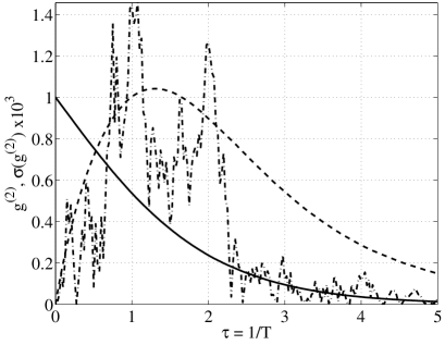
Figure 1: Second-order correlation function $g^{(2)}$ versus inverse temperature $\tau$ for $t=0$, $U=2$ and $\mu=1$, for which $\left\langle n_{j}\right\rangle=0.5$. The solid curve gives the simulation result, and the dashed and dot-dashed line show the estimated sampling error and deviation from the analytic result, respectively (on a $\times 1000$ scale). Calculated from 100,000 trajectories

Whether the method can overcome the fundamental cause of the sign problem, which is the complexity of fermionic states, must be demonstrated by calculating physical quantities in cases where the sign problem is known to occur in other methods. Thus we calculate the total energy for $t=1$, $U=4$ in two dimensions as a function of temperature, for different fillings. The results for a 16x16 lattice are shown in Fig. 2, in which to obtain good sampling with the spreading weights, we use a branching techniqueTrivediCeperley90 . For a 4x4 lattice at an inverse temperature of $\tau=7$, we calculate $E=-13.1\pm 1.2$ at $n=0.5$ and $E=-19.62\pm 0.87$ at $n=.313\pm 0.005$, which can be compared to zero-temperature, exact-diagonalisation results, namely $E=-13.62$ for $n=0.5$ (half filling) and $E=-19.57$ for $n=0.3125$ (10 atoms)Exact . At a filling of $n=0.412\pm 0.01$, for which the sign deteriorates for a projector QMC calculationFettesMorgenstern00 , we calculate $E=-16.5\pm 1.5$. We emphasise that, unlike projector QMC Linden92 , the Gaussian method can calculate any physical correlation function, at any temperature.

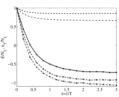
Figure 2: Total energy $E$ per site versus inverse temperature $\tau$ for a $16\times 16$ 2D lattice for chemical potentials $\mu=2$ (solid), $\mu=1$ (dashed) and $\mu=0$ (dot-dashed). Curves without crosses give the number of particles per site for $\mu=1$ (dashed) and $\mu=0$ (dot-dashed). $U=4$, $t=1$, and 50 paths initially. Dotted curves give an estimate of sampling error.

As an application of the method to a dynamical calculation, in particular to a composite Bose/Fermi system, we consider the process of the dissociation of a molecular Bose condensate into its constituent atoms, which may be fermions or bosons. For simplicity, we consider two atomic modes, representing, for example, states of different spin or momenta, coupled to a single molecular mode, via the effective interaction $\hat{H}=\hat{a}^{\dagger}\hat{b}_{1}\hat{b}_{2}+\mathrm{h.c.}$, where $\hat{b}_{j}^{\dagger}$, $\hat{b}_{j}$ are the atomic creation and annihilation operators and $\hat{a}^{\dagger}$, $\hat{a}$ are the bosonic molecular operators. Realistic models of the atomic-molecular Feshbach resonances contain such terms to describe the coupling, and it is important to illustrate how this method can represent them. Because the normal spin-spin correlations $<\hat{b}_{1}^{\dagger}\hat{b}_{2}>$ will remain zero in this system (if initially zero), the phase space of the system reduces to $\overrightarrow{\lambda}=(\alpha,\alpha^{+},n_{1,}n_{2},m,m^{+})\,\,,$ i. e. four complex atomic variables and two complex molecular amplitudes. Applying the identities in Eq. (9) and in Gauss:Bosons , we derive the following phase-space equations for the time evolution, (where $+\rightarrow\mathrm{bosonic}$, $-\rightarrow\mathrm{fermionic})$:

$$\dot{n_{j}} = i(\alpha^{+}m-\alpha m^{+})\pm\sqrt{i}n_{j}\left(m\zeta_{1}^{\ast}+m^{+}\zeta_{2}^{\ast}\right)\,\,,$$

$$\dot{m} = -i\alpha(1\pm n_{1}\pm n_{2})+\sqrt{i}\left(\pm m^{2}\zeta_{1}^{\ast}+n_{1}n_{2}\zeta_{2}^{\ast}\right)\,\,,$$

$$\dot{m^{+}} = i\alpha^{+}(1\pm n_{1}\pm n_{2})+\sqrt{i}\left(n_{1}n_{2}\zeta_{1}^{\ast}\pm m^{+2}\zeta_{2}^{\ast}\right)\,\,,$$

$$\dot{\alpha} = -im-\sqrt{i}\zeta_{1}\,\,,\,\,\dot{\alpha^{+}}=im^{+}+\sqrt{i}\zeta_{2}\,\,,$$ (13)

where $j=1,2$ and where the $\zeta_{k}(t)$ are two complex Gaussian noises, defined by the correlations $\left\langle\zeta_{k}(t)\zeta_{k^{\prime}}(t^{\prime})\right\rangle=0\,,\,\,\left\langle\zeta_{k}(t)\zeta_{k^{\prime}}^{\ast}(t^{\prime})\right\rangle=\delta_{k,k^{\prime}}\delta(t-t^{\prime})\,\,$. Simulations of Eqs. (13) are compared with truncated number-state-based calculations in Fig. 3. Although the initial rates of conversion are the same in each case, a Pauli blocking effect soon slows the fermionic conversion, in contrast to an enhanced bosonic conversion. We note that in these real-time calculations, a growing sampling error appears to be a generic property, although a prudent gauge choice may control the growth rate for a certain time.

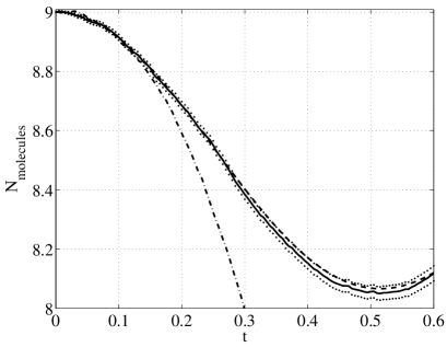
Figure 3: Molecular dissociation into pairs of fermionic (solid line) or bosonic (dot-dashed line) atoms. For the fermionic case, the dashed curve gives the truncated number-state calculation, and the dotted lines the estimated sampling error. In the bosonic case, the estimated sampling error is too small to be distinctly plotted on this graph. The initial state is a molecular coherent state ( $N_{{\rm molecules}}(0)=9$). Calculated from 10,000 trajectories.

In summary, we have introduced here an operator representation that is able to represent arbitrary physical states of fermions. Together with the corresponding bosonic representation, it is the largest class of representations that can be constructed using an operator basis that is Gaussian in the ladder operators. We have presented identities for first-principles calculations of the time evolution of quantum systems, both dynamical (real time) and canonical (imaginary time). A quadratic master equation maps to deterministic equations, whereas interacting systems with quartic terms in the Hamiltonian generate stochastic equations, provided a suitable stochastic gauge is chosen that eliminates all boundary terms. No computationally intensive determinant calculations are involved.

The simple examples given here show how the one, unified method can solve both fermionic and bosonic problems, making it well suited to simulating Bose-Fermi mixtures, and to studying from first-principles, for example, the BEC/BCS crossover. Importantly, a new type of Fermi stochastic freedom can be used to map canonical calculations of the Hubbard type onto a real subspace. We have thereby been able to numerically simulate the Hubbard model without sign error, even without employing any of the sophisticated sampling techniques that have been developed over time to optimise more conventional QMC methods. The application of such techniques to the Gaussian approach is yet to be explored.

We gratefully acknowledge support from the Australian Research Council.

References

- (1) D. M. Ceperley, Rev. Mod. Phys. 71, 438 (1999).
- (2) W. von der Linden, Phys. Rep. 220, 53 (1992).
- (3) R. R. dos Santos, Brazilian Journal of Physics 33, 36 (2003).
- (4) G. E Astrakharchik et al, cond-mat/0406113.
- (5) P. D. Drummond, P. Deuar, J. F. Corney and K. Kheruntsyan, in Proceedings of the 16th International Conference on Laser Spectroscopy, ed. P. Hannaford, A. Sidorov, H. Bachor and K. Baldwin (World Scientific, 2004), p 161.
- (6) K. E. Cahill and R. J. Glauber, Phys. Rev. A 59, 1538 (1999); L. I. Plimak, M. J. Collett and M. K. Olsen, Phys. Rev. A 64, 063409 (2001).
- (7) O. Juillet, F. Gulminelli and Ph. Chomaz, Phys. Rev. Lett. 92, 160401 (2004).
- (8) J. F. Corney and P. D. Drummond, Phys. Rev. A 68, 063822 (2003).
- (9) The square of the Pfaffian equals the determinant.
- (10) E. H. Lieb and F. Y. Wu, Phys. Rev. Lett. 20, 1445 (1968).
- (11) W. Fettes and I. Morgenstern, Computer Physics Communications 124, 148 (2000).
- (12) P. Deuar and P. D. Drummond, Comp. Phys. Comm. 142, 442 (2001); P. Deuar and P. D. Drummond, Phys. Rev. A 66, 033812 (2002); P.D. Drummond and P. Deuar, J. Opt. B 5, 281 (2003).
- (13) N. Trivedi and D. M. Ceperley, Phys. Rev. B 41, 4552 (1990).
- (14) S. Sorella, A. Parola, M. Parrinello and E. Tosatti, Europhys. Lett. 12, 721 (1990).