Abstract

General relativity may seem very different from quantum theory, but work on quantum gravity has revealed a deep analogy between the two. General relativity makes heavy use of the category $n{\rm Cob}$, whose objects are $(n-1)$-dimensional manifolds representing ‘space’ and whose morphisms are $n$-dimensional cobordisms representing ‘spacetime’. Quantum theory makes heavy use of the category ${\rm Hilb}$, whose objects are Hilbert spaces used to describe ‘states’, and whose morphisms are bounded linear operators used to describe ‘processes’. Moreover, the categories $n{\rm Cob}$ and ${\rm Hilb}$ resemble each other far more than either resembles ${\rm Set}$, the category whose objects are sets and whose morphisms are functions. In particular, both ${\rm Hilb}$ and $n{\rm Cob}$ but not ${\rm Set}$ are $\ast$-categories with a noncartesian monoidal structure. We show how this accounts for many of the famously puzzling features of quantum theory: the failure of local realism, the impossibility of duplicating quantum information, and so on. We argue that these features only seem puzzling when we try to treat ${\rm Hilb}$ as analogous to ${\rm Set}$ rather than $n{\rm Cob}$, so that quantum theory will make more sense when regarded as part of a theory of spacetime.

1 Introduction

Faced with the great challenge of reconciling general relativity and quantum theory, it is difficult to know just how deeply we need to rethink basic concepts. By now it is almost a truism that the project of quantizing gravity may force us to modify our ideas about spacetime. Could it also force us to modify our ideas about the quantum? So far this thought has appealed mainly to those who feel uneasy about quantum theory and hope to replace it by something that makes more sense. The problem is that the success and elegance of quantum theory make it hard to imagine promising replacements. Here I would like to propose another possibility, namely that quantum theory will make more sense when regarded as part of a theory of spacetime. Furthermore, I claim that we can only see this from a category-theoretic perspective — in particular, one that de-emphasizes the primary role of the category of sets and functions.

Part of the difficulty of combining general relativity and quantum theory is that they use different sorts of mathematics: one is based on objects such as manifolds, the other on objects such as Hilbert spaces. As ‘sets equipped with extra structure’, these look like very different things, so combining them in a single theory has always seemed a bit like trying to mix oil and water. However, work on topological quantum field theory theory has uncovered a deep analogy between the two. Moreover, this analogy operates at the level of categories.

We shall focus on two categories in this paper. One is the category ${\rm Hilb}$ whose objects are Hilbert spaces and whose morphisms are linear operators between these. This plays an important role in quantum theory. The other is the category $n{\rm Cob}$ whose objects are $(n-1)$-dimensional manifolds and whose morphisms are $n$-dimensional manifolds going between these. This plays an important role in relativistic theories where spacetime is assumed to be $n$-dimensional: in these theories the objects of $n{\rm Cob}$ represent possible choices of ‘space’, while the morphisms — called ‘cobordisms’ — represent possible choices of ‘spacetime’.

While an individual manifold is not very much like a Hilbert space, the category $n{\rm Cob}$ turns out to have many structural similarities to the category ${\rm Hilb}$. The goal of this paper is to explain these similarities and show that the most puzzling features of quantum theory all arise from ways in which ${\rm Hilb}$ resembles $n{\rm Cob}$ more than the category ${\rm Set}$, whose objects are sets and whose morphisms are functions.

Since sets and functions capture many basic intuitions about macroscopic objects, and the rules governing them have been incorporated into the foundations of mathematics, we naturally tend to focus on the fact that any quantum system has a set of states. From a Hilbert space we can indeed extract a set of states, namely the set of unit vectors modulo phase. However, this is often more misleading than productive, because this process does not define a well-behaved map — or more precisely, a functor — from ${\rm Hilb}$ to ${\rm Set}$. In some sense the gap between ${\rm Hilb}$ and ${\rm Set}$ is too great to be usefully bridged by this trick. However, many of the ways in which ${\rm Hilb}$ differs from ${\rm Set}$ are ways in which it resembles $n{\rm Cob}$! This suggests that the interpretation of quantum theory will become easier, not harder, when we finally succeed in merging it with general relativity.

In particular, it is easy to draw pictures of the objects and morphisms of $n{\rm Cob}$, at least for low $n$. Doing so lets us visualize many features of quantum theory. This is not really a new discovery: it is implicit in the theory of Feynman diagrams. Whenever one uses Feynman diagrams in quantum field theory, one is secretly working in some category where the morphisms are graphs with labelled edges and vertices, as shown in Figure 1.

Figure 1: A Feynman diagram

The precise details of the category depend on the quantum field theory in question: the labels for edges correspond to the various particles of the theory, while the labels for vertices correspond to the interactions of the theory. Regardless of the details, categories of this sort share many of the structural features of both $n{\rm Cob}$ and ${\rm Hilb}$. Their resemblance to $n{\rm Cob}$, namely their topological nature, makes them a powerful tool for visualization. On the other hand, their relation to ${\rm Hilb}$ makes them useful in calculations.

Though Feynman diagrams are far from new, the fact that they are morphisms in a category only became appreciated in work on quantum gravity, especially string theory and loop quantum gravity. Both these approaches stretch the Feynman diagram concept in interesting new directions. In string theory, Feynman diagrams are replaced by ‘string worldsheets’: 2-dimensional cobordisms mapped into an ambient spacetime, as shown in Figure 2. Since these cobordisms no longer have definite edges and vertices, there are no labels anymore. This is one sense in which the various particles and interactions are all unified in string theory. The realization that processes in string theory could be described as morphisms in a category was crystallized by Segal’s definition of ‘conformal field theory’ [31].

Figure 2: A string worldsheet

Loop quantum gravity is moving towards a similar picture, though with some important differences. In this approach processes are described by ‘spin foams’. These are a 2-dimensional generalization of Feynman diagrams built from vertices, edges and faces, as shown in Figure 3. They are not mapped into an ambient spacetime: in this approach spacetime is nothing but the spin foam itself — or more precisely, a linear combination of spin foams. Particles and interactions are not ‘unified’ in these models, so there are labels on the vertices, edges and faces, which depend on the details of the model in question. The category-theoretic underpinnings of spin foam models were explicit from the very beginning [4], since they were developed after Segal’s work on conformal field theory, and also after Atiyah’s work on topological quantum field theory [2], which exhibits the analogy between $n{\rm Cob}$ and ${\rm Hilb}$ in its simplest form.

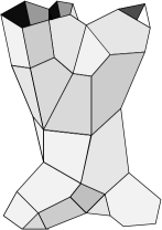
Figure 3: A spin foam

There is not one whit of experimental evidence for either string theory or loop quantum gravity, and both theories have some serious problems, so it might seem premature for philosophers to consider their implications. It indeed makes little sense for philosophers to spend time chasing every short-lived fad in these fast-moving subjects. Instead, what is worthy of reflection is that these two approaches to quantum gravity, while disagreeing heatedly on so many issues [32, 33], have so much in common. It suggests that in our attempts to reconcile the quantum-theoretic notions of state and process with the relativistic notions of space and spacetime, we have a limited supply of promising ideas. It is an open question whether these ideas will be up to the task of describing nature. But this actually makes it more urgent, not less, for philosophers to clarify and question these ideas and the implicit assumptions upon which they rest.

Before plunging ahead, let us briefly sketch the contents of this paper. In Section 2 we explain the analogy between $n{\rm Cob}$ and ${\rm Hilb}$ by recalling Atiyah’s definition of ‘topological quantum field theory’, or ‘TQFT’ for short. In Section 3, we begin by noting that unlike many familiar categories, neither ${\rm Hilb}$ nor $n{\rm Cob}$ is best regarded as a category whose objects are sets equipped with extra structures and properties, and whose morphisms are functions preserving these extra structures. In particular, operators between Hilbert spaces are not required to preserve the inner product. This raises the question of precisely what role the inner product plays in the category ${\rm Hilb}$. Of course the inner product is crucial in quantum theory, since we use it to compute transition amplitudes between states — but how does it manifest itself mathematically in the structure of ${\rm Hilb}$? One answer is that it gives a way to ‘reverse’ an operator $T\colon H\rightarrow H^{\prime}$, obtaining an operator $T^{\ast}\colon H^{\prime}\rightarrow H$ called the ‘adjoint’ of $T$ such that

$$\langle T^{\ast}\phi,\psi\rangle=\langle\phi,T\psi\rangle$$

for all $\psi\in H$ and $\phi\in H^{\prime}$. This makes ${\rm Hilb}$ into something called a ‘$\ast$-category’: a category where there is a built-in way to reverse any process. As we shall see, it is easy to compute transition amplitudes using the $\ast$-category structure of ${\rm Hilb}$. The category $n{\rm Cob}$ is also a $\ast$-category, where the adjoint of a spacetime is obtained simply by switching the roles of future and past. On the other hand, ${\rm Set}$ cannot be made into a $\ast$-category. All this suggests that both quantum theory and general relativity will be best understood in terms of categories quite different from the category of sets and functions.

In Section 4 we tackle some of the most puzzling features of quantum theory, namely those concerning joint systems: physical systems composed of two parts. It is in the study of joint systems that one sees the ‘failure of local realism’ that worried Einstein so terribly [14], and was brought into clearer focus by Bell [8]. Here is also where one discovers that one ‘cannot clone a quantum state’ — a result due to Wooters and Zurek [34] which serves as the basis of quantum cryptography. As explained in Section 4, both these phenomena follow from the failure of the tensor product to be ‘cartesian’ in a certain sense made precise by category theory. In ${\rm Set}$, the usual product of sets is cartesian, and this encapsulates many of our usual intuitions about ordered pairs, like our ability to pick out the components $a$ and $b$ of any pair $(a,b)$, and our ability to ‘duplicate’ any element $a$ to obtain a pair $(a,a)$. The fact that we cannot do these things in ${\rm Hilb}$ is responsible for the failure of local realism and the impossibility of duplicating a quantum state. Here again the category ${\rm Hilb}$ resembles $n{\rm Cob}$ more than ${\rm Set}$. Like ${\rm Hilb}$, the category $n{\rm Cob}$ has a noncartesian tensor product, given by the disjoint union of manifolds. Some of the mystery surrounding joint systems in quantum theory dissipates when one focuses on the analogy to $n{\rm Cob}$ and stops trying to analogize the tensor product of Hilbert spaces to the Cartesian product of sets.

This paper is best read as a followup to my paper ‘Higher-Dimensional Algebra and Planck-Scale Physics’ [5], since it expands on some of the ideas already on touched upon there.

2 Lessons from Topological Quantum Field Theory

Thanks to the influence of general relativity, there is a large body of theoretical physics that does not presume a fixed topology for space or spacetime. The idea is that after having assumed that spacetime is $n$-dimensional, we are in principle free to choose any $(n-1)$-dimensional manifold to represent space at a given time. Moreover, given two such manifolds, say $S$ and $S^{\prime}$, we are free to choose any $n$-dimensional manifold-with-boundary, say $M$, to represent the portion of spacetime between them, so long as the boundary of $M$ is the union of $S$ and $S^{\prime}$. In this situation we write $M\colon S\rightarrow S^{\prime}$, even though $M$ is not a function from $S$ to $S^{\prime}$, because we may think of $M$ as the process of time passing from the moment $S$ to the moment $S^{\prime}$. Mathematicians call $M$ a cobordism from $S$ to $S^{\prime}$. For example, in Figure 4 we depict a 2-dimensional manifold $M$ going from a 1-dimensional manifold $S$ (a pair of circles) to a 1-dimensional manifold $S^{\prime}$ (a single circle). Physically, this cobordism represents a process in which two separate spaces collide to form a single one! This is an example of ‘topology change’.

Figure 4: A cobordism

All this has a close analogue in quantum theory. First, just as we can use any $(n-1)$-manifold to represent space, we can use any Hilbert space to describe the states of some quantum system. Second, just as we can use any cobordism to represent a spacetime going from one space to another, we can use any operator to describe a process taking states of one system to states of another. More precisely, given systems whose states are described using the Hilbert spaces $H$ and $H^{\prime}$, respectively, any bounded linear operator $T\colon H\rightarrow H^{\prime}$ describes a process that carries states of the first system to states of the second. We are most comfortable with this idea when the operator $T$ is unitary, or at least an isometry. After all, given a state described as a unit vector $\psi\in H$, we can only be sure $T\psi$ is a unit vector in $H^{\prime}$ if $T$ is an isometry. So, only in this case does $T$ define a function from the set of states of the first system to the set of states of the second. However, the interpretation of linear operators as processes makes sense more generally. One way to make this interpretation precise is as follows: given a unit vector $\psi\in H$ and an orthonormal basis $\phi_{i}$ of $H^{\prime}$, we declare that the relative probability for a system prepared in the state $\psi$ to be observed in the state $\phi_{i}$ after undergoing the process $T$ is $|\langle\phi_{i},T\psi\rangle|^{2}$. By this, we mean that the probability of observing the system in the $i$th state divided by the probability of observing it in the $j$th state is

$$\frac{|\langle\phi_{i},T\psi\rangle|^{2}}{|\langle\phi_{j},T\psi\rangle|^{2}}.$$

The use of nonunitary operators to describe quantum processes is not new. For example, projection operators have long been used to describe processes like sending a photon through a polarizing filter. However, these examples traditionally arise when we treat part of the system (e.g. the measuring apparatus) classically. It is often assumed that at a fundamental level, the laws of nature in quantum theory describe time evolution using unitary operators. But as we shall see in Section 3, this assumption should be dropped in theories where the topology of space can change. In such theories we should let all the morphisms in ${\rm Hilb}$ qualify as ‘processes’, just as we let all morphisms in $n{\rm Cob}$ qualify as spacetimes.

Having clarified this delicate point, we are now in a position to clearly see a structural analogy between general relativity and quantum theory, in which $(n-1)$-dimensional manifolds representing space are analogous to Hilbert spaces, while cobordisms describing spacetime are analogous to operators. Indulging in some lofty rhetoric, we might say that space and state are aspects of being, while spacetime and process are aspects of becoming. We summarize this analogy in Table 1.

GENERAL RELATIVITY	QUANTUM THEORY
$(n-1)$-dimensional manifold	Hilbert space
(space)	(states)
cobordism between $(n-1)$-dimensional manifolds	operator between Hilbert spaces
(spacetime)	(process)
composition of cobordisms	composition of operators
identity cobordism	identity operator

Table 1: Analogy between general relativity and quantum theory

This analogy becomes more than mere rhetoric when applied to topological quantum field theory [5]. In quantum field theory on curved spacetime, space and spacetime are not just manifolds: they come with fixed ‘background metrics’ that allow us to measure distances and times. In this context, $S$ and $S^{\prime}$ are Riemannian manifolds, and $M\colon S\rightarrow S^{\prime}$ is a Lorentzian cobordism from $S$ to $S^{\prime}$: that is, a Lorentzian manifold with boundary whose metric restricts at the boundary to the metrics on $S$ and $S^{\prime}$. However, topological quantum field theories are an attempt to do background-free physics, so in this context we drop the background metrics: we merely assume that space is an $(n-1)$-dimensional manifold and spacetime is a cobordism between such manifolds. A topological quantum field theory then consists of a map $Z$ assigning a Hilbert space of states $Z(S)$ to any $(n-1)$-manifold $S$ and a linear operator $Z(M)\colon Z(S)\rightarrow Z(S^{\prime})$ to any cobordism between such manifolds. This map cannot be arbitrary, though: for starters, it must be a functor from the category of $n$-dimensional cobordisms to the category of Hilbert spaces. This is a great example of how every sufficiently good analogy is yearning to become a functor.

However, we are getting a bit ahead of ourselves. Before we can talk about functors, we must talk about categories. What is the category of $n$-dimensional cobordisms, and what is the category of Hilbert spaces? The answers to these questions will allow us to make the analogy in Table 1 much more precise.

First, recall that a category consists of a collection of objects, a collection of morphisms $f\colon A\rightarrow B$ from any object $A$ to any object $B$, a rule for composing morphisms $f\colon A\rightarrow B$ and $g\colon B\rightarrow C$ to obtain a morphism $gf\colon A\rightarrow C$, and for each object $A$ an identity morphism $1_{A}\colon A\rightarrow A$. These must satisfy the associative law $f(gh)=(fg)h$ and the left and right unit laws $1_{A}f=f$ and $f1_{A}=f$ whenever these composites are defined. In many cases, the objects of a category are best thought of as sets equipped with extra structure, while the morphisms are functions preserving the extra structure. However, this is true neither for the category of Hilbert spaces nor for the category of cobordisms.

In the category ${\rm Hilb}$ we take the objects to be Hilbert spaces and the morphisms to be bounded linear operators. Composition and identity operators are defined as usual. Hilbert spaces are indeed sets equipped with extra structure, but bounded linear operators do not preserve all this extra structure: in particular, they need not preserve the inner product. This may seem like a fine point, but it is important, and we shall explore its significance in detail in Section 3.

In the category $n{\rm Cob}$ we take the objects to be $(n-1)$-dimensional manifolds and the morphisms to be cobordisms between these. (For technical reasons mathematicians usually assume both to be compact and oriented.) Here the morphisms are not functions at all! Nonetheless we can ‘compose’ two cobordisms $M\colon S\rightarrow S^{\prime}$ and $M^{\prime}\colon S^{\prime}\rightarrow S^{\prime\prime}$, obtaining a cobordism $M^{\prime}M\colon S\rightarrow S^{\prime\prime}$, as in Figure 5. The idea here is that the passage of time corresponding to $M$ followed by the passage of time corresponding to $M^{\prime}$ equals the passage of time corresponding to $M^{\prime}M$. This is analogous to the familiar idea that waiting $t$ seconds followed by waiting $t^{\prime}$ seconds is the same as waiting $t^{\prime}+t$ seconds. The big difference is that in topological quantum field theory we cannot measure time in seconds, because there is no background metric available to let us count the passage of time. We can only keep track of topology change. Just as ordinary addition is associative, composition of cobordisms satisfies the associative law:

$$(M^{\prime\prime}M^{\prime})M=M^{\prime\prime}(M^{\prime}M).$$

Figure 5: Composition of cobordisms

Furthermore, for any $(n-1)$-dimensional manifold $S$ representing space, there is a cobordism $1_{S}\colon S\rightarrow S$ called the ‘identity’ cobordism, which represents a passage of time during which the topology of space stays constant. For example, when $S$ is a circle, the identity cobordism $1_{S}$ is a cylinder, as shown in Figure 6. In general, the identity cobordism $1_{S}$ has the property that

$$1_{S}M=M$$

and

$$M1_{S}=M$$

whenever these composites are defined. These properties say that an identity cobordism is analogous to waiting 0 seconds: if you wait 0 seconds and then wait $t$ more seconds, or wait $t$ seconds and then wait 0 more seconds, this is the same as waiting $t$ seconds.

Figure 6: An identity cobordism

A functor between categories is a map sending objects to objects and morphisms to morphisms, preserving composition and identities. Thus, in saying that a topological quantum field theory is a functor

$$Z\colon n{\rm Cob}\rightarrow{\rm Hilb},$$

we merely mean that it assigns a Hilbert space of states $Z(S)$ to any $(n-1)$-dimensional manifold $S$ and a linear operator $Z(M)\colon Z(S)\rightarrow Z(S^{\prime})$ to any $n$-dimensional cobordism $M\colon S\rightarrow S^{\prime}$ in such a way that:

• For any $n$-dimensional cobordisms $M\colon S\rightarrow S^{\prime}$ and $M^{\prime}\colon S^{\prime}\rightarrow S^{\prime\prime}$,

  $$Z(M^{\prime}M)=Z(M^{\prime})Z(M).$$

• For any $(n-1)$-dimensional manifold $S$,

  $$Z(1_{S})=1_{Z(S)}.$$

Both these axioms make sense if one ponders them a bit. The first says that the passage of time corresponding to the cobordism $M$ followed by the passage of time corresponding to $M^{\prime}$ has the same effect on a state as the combined passage of time corresponding to $M^{\prime}M$. The second says that a passage of time in which no topology change occurs has no effect at all on the state of the universe. This seems paradoxical at first, since it seems we regularly observe things happening even in the absence of topology change. However, this paradox is easily resolved: a topological quantum field theory describes a world without local degrees of freedom. In such a world, nothing local happens, so the state of the universe can only change when the topology of space itself changes.

Unless elementary particles are wormhole ends or some other sort of topological phenomenon, it seems our own world is quite unlike this. Thus, we hasten to reassure the reader that this peculiarity of topological quantum field theory is not crucial to our overall point, which is the analogy between categories describing space and spacetime and those describing quantum states and processes. If we were doing quantum field theory on curved spacetime, we would replace $n{\rm Cob}$ with a category where the objects are $n$-dimensional Riemannian manifolds and most of the morphisms are Lorentzian cobordisms between these. In this case a cobordism $M\colon S\rightarrow S^{\prime}$ has not just a topology but also a geometry, so we can use cylinder-shaped cobordisms of different ‘lengths’ to describe time evolution for different amounts of time. The identity morphism is then described by a cylinder of ‘length zero’. This degenerate cylinder is not really a Lorentzian cobordism, which leads to some technical complications. However, Segal showed how to get around these in his axioms for a conformal field theory [31]. There are some further technical complications arising from the fact that except in low dimensions, we need to use the C*-algebraic approach to quantum theory, instead of the Hilbert space approach [13]. Here the category ${\rm Hilb}$ should be replaced by one where the objects are C^∗-algebras and the morphisms are completely positive maps between their duals [15].

Setting aside these nuances, our main point is that treating a TQFT as a functor from $n{\rm Cob}$ to ${\rm Hilb}$ is a way of making very precise some of the analogies between general relativity and quantum theory. However, we can go further! A TQFT is more than just a functor. It must also be compatible with the ‘monoidal category’ structure of $n{\rm Cob}$ and ${\rm Hilb}$, and to be physically well-behaved it must also be compatible with their ‘$\ast$-category’ structure. We examine these extra structures in the next two sections.

3 The $\ast$-Category of Hilbert Spaces

What is the category of Hilbert spaces? While we have already given an answer, this is actually a tricky question, one that makes many category theorists acutely uncomfortable.

To understand this, we must start by recalling that one use of categories is to organize discourse about various sorts of ‘mathematical objects’: groups, rings, vector spaces, topological spaces, manifolds and so on. Quite commonly these mathematical objects are sets equipped with extra structure and properties, so let us restrict attention to this case. Here by structure we mean operations and relations defined on the set in question, while by properties we mean axioms that these operations and relations are required to satisfy. The division into structure and properties is evident from the standard form of mathematical definitions such as “a widget is a set equipped with … such that ….” Here the structures are listed in the first blank, while the properties are listed in the second.

To build a category of this sort of mathematical object, we must also define morphisms between these objects. When the objects are sets equipped with extra structure and properties, the morphisms are typically taken to be functions that preserve the extra structure. At the expense of a long digression we could make this completely precise — and also more general, since we can also build categories by equipping not sets but objects of other categories with extra structure and properties. However, we prefer to illustrate the idea with an example. We take an example closely related to but subtly different from the category of Hilbert spaces: the category of complex vector spaces.

A complex vector space is a set $V$ equipped with extra structure consisting of operations called addition

$$+\colon V\times V\rightarrow V$$

and scalar multiplication

$$\cdot\colon{\mathbb{C}}\times V\rightarrow V,$$

which in turn must have certain extra properties: commutativity and associativity together with the existence of an identity and inverses for addition, associativity and the unit law for scalar multiplication, and distributivity of scalar multiplication over adddition. Given vector spaces $V$ and $V^{\prime}$, a linear operator $T\colon V\rightarrow V^{\prime}$ can be defined as a function preserving all the extra structure. This means that we require

$$T(\psi+\phi)=T(\psi)+T(\phi)$$

and

$$T(c\psi)=cT(\psi)$$

for all $\psi,\phi\in V$ and $c\in{\mathbb{C}}$. Note that the properties do not enter here. Mathematicians define the category ${\rm Vect}$ to have complex vector spaces as its objects and linear operators between them as its morphisms.

Now compare the case of Hilbert spaces. A Hilbert space $H$ is a set equipped with all the structure of a complex vector space but also some more, namely an inner product

$$\langle\cdot,\cdot\rangle\colon H\times H\rightarrow{\mathbb{C}}.$$

Similarly, it has all the properties of a complex vector spaces but also some more: for all $\phi,\psi,\psi^{\prime}\in H$ and $c\in{\mathbb{C}}$ we have the equations

$$\langle\phi,\psi+\psi^{\prime}\rangle=\langle\phi,\psi\rangle+\langle\phi,\psi^{\prime}\rangle,$$

$$\langle\phi,c\psi\rangle=c\langle\phi,\psi\rangle,$$

$$\langle\phi,\psi\rangle=\overline{\langle\psi,\phi\rangle},$$

together with the inequality

$$\langle\psi,\psi\rangle\geq 0$$

where equality holds only if $\psi=0$; furthermore, the norm defined by the inner product must be complete. Given Hilbert spaces $H$ and $H^{\prime}$, a function $T\colon H\rightarrow H^{\prime}$ that preserves all the structure is thus a linear operator that preserves the inner product:

$$\langle T\phi,T\psi\rangle=\langle\phi,\psi\rangle$$

for all $\phi,\psi\in H$. Such an operator is called an isometry.

If we followed the pattern that works for vector spaces and many other mathematical objects, we would thus define the category ${\rm Hilb}$ to have Hilbert spaces as objects and isometries as morphisms. However, this category seems too constricted to suit what physicists actually do with Hilbert spaces: they frequently need operators that aren’t isometries! Unitary operators are always isometries, but self-adjoint operators, for example, are not.

The alternative we adopt in this paper is to work with the category ${\rm Hilb}$ whose objects are Hilbert spaces and the morphisms are bounded linear operators. However, this leads to a curious puzzle. In a precise technical sense, the category of finite-dimensional Hilbert spaces and linear operators between these is equivalent to the category of finite-dimensional complex vector spaces and linear operators. So, in defining this category, we might as well ignore the inner product entirely! The puzzle is thus what role, if any, the inner product plays in this category.

The case of general, possibly infinite-dimensional Hilbert spaces is subtler, but the puzzle persists. The category of all Hilbert spaces and bounded linear operators between them is not equivalent to the category of all complex vector spaces and linear operators. However, it is equivalent to the category of ‘Hilbertizable’ vector spaces — that is, vector spaces equipped with a topology coming from some Hilbert space structure — and continuous linear operators between these. So, in defining this category, what matters is not the inner product but merely the topology it gives rise to. The point is that bounded linear operators don’t preserve the inner product, just the topology, and a structure that is not preserved might as well be ignored, as far as the category is concerned.

My resolution of this puzzle is simple but a bit upsetting to most category theorists. I admit that the inner product is inessential in defining the category of Hilbert spaces and bounded linear operators. However, I insist that it plays a crucial role in making this category into a $\ast$-category!

What is a $\ast$-category? It is a category $C$ equipped with a map sending each morphism $f\colon X\rightarrow Y$ to a morphism $f^{\ast}\colon Y\rightarrow X$, satisfying

$$1_{X}^{\ast}=1_{X},$$

$$(fg)^{\ast}=g^{\ast}f^{\ast},$$

and

$$f^{\ast\ast}=f.$$

To make ${\rm Hilb}$ into a $\ast$-category we define $T^{\ast}$ for any bounded linear operator $T\colon H\rightarrow H^{\prime}$ to be the adjoint operator $T^{\ast}H^{\prime}\rightarrow H$, given by

$$\langle T^{\ast}\psi,\phi\rangle=\langle\psi,T\phi\rangle.$$

We see by this formula that the inner product on both $H$ and $H^{\prime}$ are required to define the adjoint of $T$.

In fact, we can completely recover the inner product on every Hilbert space from the $\ast$-category structure of ${\rm Hilb}$. Given a Hilbert space $H$ and a vector $\psi\in H$, there is a unique operator $T_{\psi}\colon{\mathbb{C}}\rightarrow H$ with $T_{\psi}(1)=\psi$. Conversely, any operator from ${\mathbb{C}}$ to $H$ determines a unique vector in $H$ this way. So, we can think of elements of a Hilbert space as morphisms from ${\mathbb{C}}$ to this Hilbert space. Using this trick, an easy calculation shows that

$$\langle\phi,\psi\rangle={T_{\phi}}^{\!\!\ast}\,T_{\psi}.$$

The right-hand side is really a linear operator from ${\mathbb{C}}$ to ${\mathbb{C}}$, but there is a canonical way to identify such a thing with a complex number. So, everything about inner products is encoded in the $\ast$-category structure of ${\rm Hilb}$. Moreover, this way of thinking about the inner product formalizes an old idea of Dirac. The operator $T_{\psi}$ is really just Dirac’s ‘ket’ $|\psi\rangle$, while ${T_{\phi}}^{\!\!\ast}$ is the ‘bra’ $\langle\phi|$. Composing a ket with a bra, we get the inner product.

This shows how adjoints are closely tied to the inner product structure on Hilbert space. But what is the physical significance of the adjoint of an operator, or more generally the $\ast$ operation in any $\ast$-category? Most fundamentally, the $\ast$ operation gives us a way to ‘reverse’ a morphism even when it is not invertible. If we think of inner products as giving transition amplitudes between states in quantum theory, the equation $\langle T^{\ast}\phi,\psi\rangle=\langle\phi,T\psi\rangle$ says that $T^{\ast}$ is the unique operation we can perform on any state $\phi$ so that the transition amplitude from $T\psi$ to $\phi$ is the same as that from $\psi$ to $T^{\ast}\phi$. So, in a suggestive but loose way, we can say that the process described by $T^{\ast}$ is some sort of ‘time-reversed’ version of the process described by $T$. If $T$ is unitary, $T^{\ast}$ is just the inverse of $T$. But, $T^{\ast}$ makes sense even when $T$ has no inverse!

This suggestive but loose relation between $\ast$ operations and time reversal becomes more precise in the case of $n{\rm Cob}$. Here the $\ast$ operation really is time reversal. More precisely, given an $n$-dimensional cobordism $M\colon S\rightarrow S^{\prime}$, we let the adjoint cobordism $M^{\ast}\colon S^{\prime}\rightarrow S$ to be the same manifold, but with the ‘past’ and ‘future’ parts of its boundary switched, as in Figure 7. It is easy to check that this makes $n{\rm Cob}$ into a $\ast$-category.

            

Figure 7: A cobordism and its adjoint

In a so-called unitary topological quantum field theory (the terminology is a bit unfortunate), we demand that the functor $Z\colon n{\rm Cob}\rightarrow{\rm Hilb}$ preserve the $\ast$-category structure in the following sense:

$$Z(M^{\ast})=Z(M)^{\ast}.$$

All the TQFTs of interest in physics have this property, and a similar property holds for conformal field theories and other quantum field theories on curved spacetime. This means that in the analogy between general relativity and quantum theory, the analogue of time reversal is taking the adjoint of an operator between Hilbert spaces. To ‘reverse’ a spacetime $M\colon S\rightarrow S^{\prime}$ we formally switch the notions of future and past, while to ‘reverse’ a process $T\colon H\rightarrow H^{\prime}$ we take its adjoint.

Taking this analogy seriously leads us in some interesting directions. First, since the $\ast$ operation in $n{\rm Cob}$ is given by time reversal, while $\ast$ operation in ${\rm Hilb}$ is defined using the inner product, there should be some relation between time reversal and the inner product in quantum theory! The details remain obscure, at least to me, but we can make a little progress by pondering the following equation, which we originally introduced as a ‘trick’ for expressing inner products in terms of adjoint operators:

$$\langle\phi,\psi\rangle={T_{\phi}}^{\!\!\ast}\,T_{\psi}.$$

An equation this important should not be a mere trick! To try to interpret it, suppose that in some sense the operator $T_{\psi}$ describes ‘the process of preparing the system to be in the state $\psi$’, while ${T_{\phi}}^{\!\!\ast}$ describes the process of ‘observing the system to be in the state $\phi$’. Given this, ${T_{\phi}}^{\!\!\ast}\,T_{\psi}$ should describe the process of first preparing the system to be in the state $\psi$ and then observing it to be in the state $\phi$. The above equation then relates this composite process to the transition amplitude $\langle\phi,\psi\rangle$. Moreover, we see that ‘observation’ is like a time-reversed version of ‘preparation’. All this makes a rough intuitive kind of sense. However, these ideas could use a great deal of elaboration and clarification. I mention them here mainly to open an avenue for further thought.

Second, and less speculatively, the equation $Z(M^{\ast})=Z(M)^{\ast}$ sheds some light on the relation between topology change and the failure of unitarity, mentioned already in Section 2. In any $\ast$-category, we may define a morphism $f\colon x\rightarrow y$ to be unitary if $f^{\ast}f=1_{x}$ and $ff^{\ast}=1_{y}$. For a morphism in ${\rm Hilb}$ this reduces to the usual definition of unitarity for a linear operator. One can show that a morphism $M$ in $n{\rm Cob}$ is unitary if $M$ involves no topology change, or more precisely, if $M$ is diffeomorphic to the Cartesian product of an interval and some $(n-1)$-dimensional manifold. (The converse is true in dimensions $n\leq 3$, but it fails in higher dimensions.) A TQFT satisfying $Z(M^{\ast})=Z(M)^{\ast}$ maps unitary morphisms in $n{\rm Cob}$ to unitary morphisms in ${\rm Hilb}$, so for TQFTs of this sort, absence of topology change implies unitary time evolution. This fact reinforces a point already well-known from quantum field theory on curved spacetime, namely that unitary time evolution is not a built-in feature of quantum theory but rather the consequence of specific assumptions about the nature of spacetime [13].

To conclude, it is interesting to contrast $n{\rm Cob}$ and ${\rm Hilb}$ with the more familiar category ${\rm Set}$, whose objects are sets and whose morphisms are functions. There is no way to make ${\rm Set}$ into a $\ast$-category, since there is no way to ‘reverse’ the map from the empty set to the one-element set. So, our intuitions about sets and functions help us very little in understanding $\ast$-categories. The problem is that the concept of function is based on an intuitive notion of process that is asymmetrical with respect to past and future: a function $f\colon S\rightarrow S^{\prime}$ is a relation such that each element of $S$ is related to exactly one element of $S^{\prime}$, but not necessarily vice versa. For better or worse, this built-in ‘arrow of time’ has no place in the basic concepts of quantum theory.

Pondering this, it soon becomes apparent that if we want an easy example of a $\ast$-category other than ${\rm Hilb}$ to help build our intuitions about $\ast$-categories, we should use not ${\rm Set}$ but ${\rm Rel}$, the category of sets and relations. In fact, quantum theory can be seen as a modified version of the theory of relations in which Boolean algebra has been replaced by the algebra of complex numbers! To see this, note that a linear operator between two Hilbert spaces can be described using a matrix of complex numbers as soon as we pick an orthonormal basis for each. Similarly, a relation $R$ between sets $S$ and $S^{\prime}$ can be described by a matrix of truth values, namely the truth values of the propositions $yRx$ where $x\in S$ and $y\in S^{\prime}$. Composition of relations can be defined as matrix multiplication with ‘or’ and ‘and’ playing the roles of ‘plus’ and ‘times’. It easy to check that this is associative and has an identity morphism for each set, so we obtain a category ${\rm Rel}$ with sets as objects and relations as morphisms. Furthermore, ${\rm Rel}$ becomes a $\ast$-category if we define the relation $R^{\ast}$ by saying that $xR^{\ast}y$ if and only if $yRx$. Just as the matrix for the linear operator $T^{\ast}$ is the conjugate transpose of the matrix for $T$, the matrix for the relation $R^{\ast}$ is the transpose of the matrix for $R$.

So, the category of Hilbert spaces closely resembles the category of relations. The main difference is that binary truth values describing whether or not a transition is possible are replaced by complex numbers describing the amplitude with which a transition occurs. Comparisons between ${\rm Hilb}$ and ${\rm Rel}$ are fruitful source of intuitions not only about $\ast$-categories in general but also about the meaning of ‘matrix mechanics’. For some further explorations along these lines, see the work of Abramsky and Coecke [1].

4 The Monoidal Category of Hilbert Spaces

An important goal of the enterprise of physics is to describe, not just one physical system at a time, but also how a large complicated system can be built out of smaller simpler ones. The simplest case is a so-called ‘joint system’: a system built out of two separate parts. Our experience with the everyday world leads us to believe that to specify the state of a joint system, it is necessary and sufficient to specify states of its two parts. (Here and in what follows, by ‘states’ we always mean what physicists call ‘pure states’.) In other words, a state of the joint system is just an ordered pair of states of its parts. So, if the first part has $S$ as its set of states, and the second part has $T$ as its set of states, the joint system has the cartesian product $S\times T$ as its set of states.

One of the more shocking discoveries of the twentieth century is that this is wrong. In both classical and quantum physics, given states of each part we get a state of the joint system. But only in classical physics is every state of the joint system of this form! In quantum physics are also ‘entangled’ states, which can only be described as superpositions of states of this form. The reason is that in quantum theory, the states of a system are no longer described by a set, but by a Hilbert space. Moreover — and this is really an extra assumption — the states of a joint system are described not by the cartesian product of Hilbert spaces, but by their tensor product.

Quite generally, we can imagine using objects in any category to describe physical systems, and morphisms between these to describe processes. In order to handle joint systems, this category will need to have some sort of ‘tensor product’ that gives an object $A\otimes B$ for any pair of objects $A$ and $B$. As we shall explain, categories of this sort are called ‘monoidal’. The category ${\rm Set}$ is a example where the tensor product is just the usual cartesian product of sets. Similarly, the category ${\rm Hilb}$ is a monoidal category where the tensor product is the usual tensor product of Hilbert spaces. However, these two examples are very different, because the product in ${\rm Set}$ is ‘cartesian’ in a certain technical sense, while the product in ${\rm Hilb}$ is not. This turns out to explain a lot about why joint systems behave so counterintuively in quantum physics. Moreover, it is yet another way in which ${\rm Hilb}$ resembles $n{\rm Cob}$ more than ${\rm Set}$.

To see this in detail, it pays to go back to the beginning and think about cartesian products. Given two sets $S$ and $T$, we define $S\times T$ to be the set of all ordered pairs $(s,t)$ with $s\in S$ and $t\in T$. But what is an ordered pair? This depends on our approach to set theory. We can use axioms in which ordered pairs are a primitive construction, or we can define them in terms of other concepts. For example, in 1914, Wiener defined the ordered pair $(s,t)$ to be the set $\{\{\{s\},\emptyset\},\{\{t\}\}$. In 1922, Kuratowski gave the simpler definition $(s,t)=\{\{s\},\{s,t\}\}$. We can use the still simpler definition $(s,t)=\{s,\{s,t\}\}$ if our axioms exclude the possibility of sets that contain themselves. Various other definitions have also been tried [17]. In traditional set theory we arbitrarily choose one approach to ordered pairs and then stick with it. Apart from issues of convenience or elegance, it does not matter which we choose, so long as it ‘gets the job done’. In other words, all these approaches are all just technical tricks for implementing our goal, which is to make sure that $(s,t)=(s^{\prime},t^{\prime})$ if and only if $s=s^{\prime}$ and $t=t^{\prime}$.

It is a bit annoying that the definition of ordered pair cannot get straight to the point and capture the concept without recourse to an arbitrary trick. It is natural to seek an approach that focuses more on the structural role of ordered pairs in mathematics and less on their implementation. This is what category theory provides.

The reason traditional set theory arbitarily chooses a specific implementation of the ordered pair concept is that it seems difficult to speak precisely about “some thing $(s,t)$ — I don’t care what it is — with the property that $(s,t)=(s^{\prime},t^{\prime})$ iff $s=s^{\prime}$ and $t=t^{\prime}$”. So, the first move in category theory is to stop focussing on ordered pairs and instead focus on cartesian products of sets. What properties should the cartesian product $S\times T$ have? To make our answer applicable not just to sets but to objects of other categories, it should not refer to elements of $S\times T$. So, the second move in category theory is to describe the cartesian product $S\times T$ in terms of functions to and from this set.

The cartesian product $S\times T$ has functions called ‘projections’ to the sets $S$ and $T$:

$$p_{1}\colon S\times T\rightarrow S,\qquad p_{2}\colon S\times T\rightarrow T.$$

Secretly we know that these pick out the first or second component of any ordered pair in $S\times T$:

$$p_{1}(s,t)=s,\qquad p_{2}(s,t)=t.$$

But, our goal is to characterize the product by means of these projections without explicit reference to ordered pairs. For this, the key property of the projections is that given any element $s\in S$ and any element $t\in T$, there exists a unique element $x\in S\times T$ such that $p_{1}(x)=s$ and $p_{2}(x)=T$. Furthermore, as a substitute for elements of the sets $S$ and $T$, we can use functions from an arbitrary set to these sets.

Thus, given two sets $S$ and $T$, we define their cartesian product to be any set $S\times T$ equipped with functions $p_{1}\colon S\times T\rightarrow S$, $p_{2}\colon S\times T\rightarrow T$ such that for any set $X$ and functions $f_{1}\colon X\rightarrow S$, $f_{2}\colon X\rightarrow T$, there exists a unique function $f\colon X\rightarrow S\times T$ with

$$f_{1}=p_{1}f,\qquad f_{2}=p_{2}f.$$

Note that with this definition, the cartesian product is not unique! Wiener’s definition of ordered pairs gives a cartesian product of the sets $S$ and $T$, but so does Kuratowski’s, and so does any other definition that ‘gets the job done’. However, this does not lead to any confusion, since one can easily show that any two choices of cartesian product are isomorphic in a canonical way. For a proof of this and other facts about cartesian products, see for example the textbook by McLarty [29].

All this generalizes painlessly to an arbitrary category. Given two objects $A$ and $B$ in some category, we define their cartesian product (or simply product) to be any object $A\times B$ equipped with morphisms

$$p_{1}\colon A\times B\rightarrow A,\qquad p_{2}\colon A\times B\rightarrow B,$$

called projections, such that for any object $X$ and morphisms $f_{1}\colon X\rightarrow A$, $f_{2}\colon X\rightarrow B$, there is a unique morphism $f\colon X\rightarrow A\times B$ with $f_{1}=p_{1}f$ and $f_{2}=p_{2}f$. The product may not exist, and it may not be unique, but it is unique up to a canonical isomorphism. Category theorists therefore feel free to speak of ‘the’ product when it exists.

We say a category has binary products if every pair of objects has a a product. One can also talk about $n$-ary products for other values of $n$, but a category with binary products has $n$-ary products for all $n\geq 1$, since we can construct these as iterated binary products. The case $n=1$ is trivial, since the product of one object is just that object itself (up to canonical isomorphism). The only remaining case is $n=0$. This is surprisingly important. A $0$-ary product is usually called a terminal object and denoted $1$: it is an object such that that for any object $X$ there exists a unique morphism from $X$ to $1$. Terminal objects are unique up to canonical isomorphism, so we feel free to speak of ‘the’ terminal object in a category when one exists. The reason we denote the terminal object by $1$ is that in ${\rm Set}$, any set with one element is a terminal object. If a category has a terminal object and binary products, it has $n$-ary products for all $n$, so we say it has finite products.

It turns out that these concepts capture much of our intuition about joint systems in classical physics. In the most stripped-down version of classical physics, the states of a system are described as elements of a mere set. In more elaborate versions, the states of a system form an object in some fancier category, such as the category of topological spaces or manifolds. But, just like ${\rm Set}$, these fancier categories have finite products — and we use this fact when describing the states of a joint system.

To sketch how this works in general, suppose we have any category with finite products. To do physics with this, we think of any of the objects of this category as describing some physical system. It sounds a bit vague to say that a physical system is ‘described by’ some object $A$, but we can make this more precise by saying that states of this system are morphisms $f\colon 1\rightarrow A$. When our category is ${\rm Set}$, a morphism of this sort simply picks out an element of the set $A$. In the category of topological spaces, a morphism of this sort picks out a point in the topological space $A$ — and similarly for the category of manifolds, and so on. For this reason, category theorists call a morphism $f\colon 1\rightarrow A$ an element of the object $A$.

Next, we think of any morphism $g\colon A\rightarrow B$ as a ‘process’ carrying states of the system described by $A$ to states of the system described by $B$. This works as follows: given a state of the first system, say $f\colon 1\rightarrow A$, we can compose it with $g$ to get a state of the second system, $gf\colon 1\rightarrow B$.

Then, given two systems that are described by the objects $A$ and $B$, respectively, we decree that the joint system built from these is described by the object $A\times B$. The projection $p_{1}\colon A\times B\rightarrow A$ can be thought of as a process that takes a state of the joint system and discards all information about the second part, retaining only the state of the first part. Similarly, the projection $p_{2}$ retains only information about the second part.

Calling these projections ‘processes’ may strike the reader as strange, since ‘discarding information’ sounds like a subjective change of our description of the system, rather than an objective physical process like time evolution. However, it is worth noting that in special relativity, time evolution corresponds to a change of coordinates $t\mapsto t+c$, which can also be thought of as change of our description of the system. The novelty in thinking of a projection as a physical process really comes, not from the fact that it is ‘subjective’, but from the fact that it is not invertible.

With this groundwork laid, we can use the definition of ‘product’ to show that a state of a joint system is just an ordered pair of states of each part. First suppose we have states of each part, say $f_{1}\colon 1\rightarrow A$ and $f_{2}\colon 1\rightarrow B$. Then there is a unique state of the joint system, say $f\colon 1\rightarrow A\times B$, which reduces to the given state of each part when we discard information about the other part: $p_{1}f=f_{1}$ and $p_{2}f=f_{2}$. Conversely, every state of the joint system arises this way, since given $f\colon 1\rightarrow A\times B$ we can recover $f_{1}$ and $f_{2}$ using these equations.

However, the situation changes drastically when we switch to quantum theory! The states of a quantum system can still be thought of as forming a set. However, we do not take the product of these sets to be the set of states for a joint quantum system. Instead, we describe states of a system as unit vectors in a Hilbert space, modulo phase. We define the Hilbert space for a joint system to be the tensor product of the Hilbert spaces for its parts.

The tensor product of Hilbert spaces is not a cartesian product in the sense defined above, since given Hilbert spaces $H$ and $K$ there are no linear operators $p_{1}\colon H\otimes K\rightarrow H$ and $p_{2}\colon H\otimes K\rightarrow K$ with the required properties. This means that from a (pure) state of a joint quantum system we cannot extract (pure) states of its parts. This is the key to Bell’s ‘failure of local realism’. Indeed, under quite general conditions one can derive Bell’s inequality from the assumption that pure states of a joint system determine pure states of its parts [3, 8], so violations of Bell’s inequality should be seen as an indication that this assumption fails.

The Wooters–Zurek argument that ‘one cannot clone a quantum state’ [34] is also based on the fact that the tensor product of Hilbert spaces is not cartesian. To get some sense of this, note that whenever $A$ is an object in some category for which the product $A\times A$ exists, there is a unique morphism

$$\Delta\colon A\rightarrow A\times A$$

such that $p_{1}\Delta=1_{A}$ and $p_{2}\Delta=1_{A}$. This morphism is called the diagonal of $A$, since in the category of sets it is the map given by $\Delta(a)=(a,a)$ for all $a\in A$, whose graph is a diagonal line when $A$ is the set of real numbers. Conceptually, the role of a diagonal morphism is to duplicate information, just as the projections discard information. In applications to physics, the equations $p_{1}\Delta=1_{A}$ and $p_{2}\Delta=1_{A}$ says that if we duplicate a state in $A$ and then discard one of the two resulting copies, we are left with a copy identical to the original.

In ${\rm Hilb}$, however, since the tensor product is not a product in the category-theoretic sense, it makes no sense to speak of a diagonal morphism $\Delta\colon H\rightarrow H\otimes H$. In fact, a stronger statement is true: there is no natural (i.e. basis-independent) way to choose a linear operator from $H$ to $H\otimes H$ other than the zero operator. So, there is no way to duplicate information in quantum theory.

Since the tensor product is not a cartesian product in the sense explained above, what exactly is it? To answer this, we need the definition of a ‘monoidal category’. Monoidal categories were introduced by Mac Lane [25] in early 1960s, precisely in order to capture those features common to all categories equipped with a well-behaved but not necessarily cartesian product. Since the definition is a bit long, let us first present it and then discuss it:

Definition. A monoidal category consists of:

(i)

a category ${\cal M}$,

(ii)

a functor $\otimes\colon{\cal M}\times{\cal M}\rightarrow{\cal M}$,

(iii)

a unit object $I\in{\cal M}$,

(iv)

natural isomorphisms called the associator:

$$a_{A,B,C}\colon(A\otimes B)\otimes C\rightarrow A\otimes(B\otimes C),$$

the left unit law:

$$\ell_{A}\colon I\otimes A\rightarrow A,$$

and the right unit law:

$$r_{A}\colon A\otimes I\rightarrow A,$$

such that the following diagrams commute for all objects $A,B,C,D\in{\cal M}$:

(v)

(vi)

This obviously requires some explanation! First, it makes use of some notions we have not explained yet, ruining our otherwise admirably self-contained treatment of category theory. For example, what is ${\cal M}\times{\cal M}$ in clause (ii) of the definition? This is just the category whose objects are pairs of objects in ${\cal M}$, and whose morphisms are pairs of morphisms in ${\cal M}$, with composition of morphisms done componentwise. So, when we say that the tensor product is a functor $\otimes\colon{\cal M}\times{\cal M}\rightarrow{\cal M}$, this implies that for any pair of objects $x,y\in{\cal M}$ there is an object $x\otimes y\in{\cal M}$, while for any pair of morphisms $f\colon x\rightarrow x^{\prime},g\colon y\rightarrow y^{\prime}$ in ${\cal M}$ there is a morphism $f\otimes g\colon x\otimes y\rightarrow x^{\prime}\otimes y^{\prime}$ in ${\cal M}$. Morphisms are just as important as objects! For example, in ${\rm Hilb}$, not only can we take the tensor product of Hilbert spaces, but also we can take the tensor product of bounded linear operators $S\colon H\rightarrow H^{\prime}$ and $T\colon K\rightarrow K^{\prime}$, obtaining a bounded linear operator

$$S\otimes T\colon H\otimes K\rightarrow H^{\prime}\otimes K^{\prime}.$$

In physics, we think of $S\otimes T$ as a joint process built from the processes $S$ and $T$ ‘running in parallel’. For example, if we have a joint quantum system whose two parts evolve in time without interacting, any time evolution operator for the whole system is given by the tensor product of time evolution operators for the two parts.

                  

Figure 8: Two cobordisms and their tensor product

Similarly, in $n{\rm Cob}$ the tensor product is given by disjoint union, both for objects and for morphisms. In Figure 8 we show two spacetimes $M$ and $M^{\prime}$ and their tensor product $M\otimes M^{\prime}$. This as a way of letting two spacetimes ‘run in parallel’, like independently evolving separate universes. The resemblance to the tensor product of morphisms in ${\rm Hilb}$ should be clear. Just as in ${\rm Hilb}$, the tensor product in $n{\rm Cob}$ is not a cartesian product: there are no projections with the required properties. There is also no natural choice of a cobordism from $S$ to $S\otimes S$. This means that the very nature of topology prevents us from finding spacetimes that ‘discard’ part of space, or ‘duplicate’ space. Seen in this light, the fact that we cannot discard or duplicate information in quantum theory is not a flaw or peculiarity of this theory. It is a further reflection of the deep structural analogy between quantum theory and the conception of spacetime embodied in general relativity.

Turning to clause (iii) in the definition, we see that a monoidal category needs to have a ‘unit object’ $I$. This serves as the multiplicative identity for the tensor product, at least up to isomorphism: as we shall see in the next clause, $I\otimes A\cong A$ and $A\otimes I\cong A$ for every object $A\in{\cal M}$. In ${\rm Hilb}$ the unit object is ${\mathbb{C}}$ regarded as a Hilbert space, while in $n{\rm Cob}$ it is the empty set regarded as an $(n-1)$-dimensional manifold. Any category with finite products gives a monoidal category in which the unit object is the terminal object $1$.

This raises an interesting point of comparison. In classical physics we describe systems using objects in a category with finite products, and a state of the system corresponding to the object $A$ is just a morphism $f\colon 1\rightarrow A$. In quantum physics we describe systems using Hilbert spaces. Is a state of the system corresponding to the Hilbert space $H$ the same as a bounded linear operator $T\colon{\mathbb{C}}\rightarrow H$? Almost, but not quite! As we saw in Section 3, such operators are in one-to-one correspondence with vectors in $H$: any vector $\psi\in H$ corresponds to an operator $T_{\psi}\colon{\mathbb{C}}\rightarrow H$ with $T_{\psi}(1)=\psi$. States, on the other hand, are the same as unit vectors modulo phase. Any nonzero vector in $H$ gives a state after we normalize it, but different vectors can give the same state, and the zero vector does not give a state at all. So, quantum physics is really different from classical physics in this way: we cannot define states as morphisms from the unit object. Nonetheless, we have seen that the morphisms $T\colon{\mathbb{C}}\rightarrow H$ play a fundamental role in quantum theory: they are just Dirac’s ‘kets’.

Next, let us ponder clause (iv) of the definition of monoidal category. Here we see that the tensor product is associative, but only up to a specified isomorphism, called the ‘associator’. For example, in ${\rm Hilb}$ we do not have $(H\otimes K)\otimes L=H\otimes(K\otimes L)$, but there is an obvious isomorphism

$$a_{H,K,L}\colon(H\otimes K)\otimes L\rightarrow H\otimes(K\otimes L)$$

given by

$$a_{H,K,L}((\psi\otimes\phi)\otimes\eta)=\psi\otimes(\phi\otimes\eta).$$

Similarly, we do not have ${\mathbb{C}}\otimes H=H$ and $H\otimes{\mathbb{C}}=H$, but there are obvious isomorphisms

$$\ell_{H}\colon{\mathbb{C}}\otimes H\rightarrow H,\qquad r_{H}\colon H\otimes{\mathbb{C}}\rightarrow H.$$

Moreover, all these isomorphisms are ‘natural’ in a precise sense. For example, when we say the associator is natural, we mean that for any bounded linear operators $S\colon H\rightarrow H^{\prime}$, $T\colon K\rightarrow K^{\prime}$, $U\colon L\rightarrow L^{\prime}$ the following square diagram commutes:

In other words, composing the top morphism with the right-hand one gives the same result as composing the left-hand one with the bottom one. This compatibility condition expresses the fact that no arbitrary choices are required to define the associator: in particular, it is defined in a basis-independent manner. Similar but simpler ‘naturality squares’ must commute for the left and right unit laws.

Finally, what about clauses (v) and (vi) in the definition of monoidal category? These are so-called ‘coherence laws’, which let us manipulate isomorphisms with the same ease as if they were equations. Repeated use of the associator lets us construct an isomorphism from any parenthesization of a tensor product of objects to any other parenthesization — for example, from $((A\otimes B)\otimes C)\otimes D$ to $A\otimes(B\otimes(C\otimes D))$. However, we can actually construct many such isomorphisms — and in this example, the pentagonal diagram in clause (v) shows two. We would like to be sure that all such isomorphisms from one parenthesization to another are equal. In his fundamental paper on monoidal categories, Mac Lane [25] showed that the commuting pentagon in clause (v) guarantees this, not just for a tensor product of four objects, but for arbitrarily many. He also showed that clause (vi) gives a similar guarantee for isomorphisms constructed using the left and right unit laws.

5 Conclusions

Our basic intuitions about mathematics are to some extent abstracted from our dealings with the everyday physical world [19]. The concept of a set, for example, formalizes some of our intuitions about piles of pebbles, herds of sheep and the like. These things are all pretty well described by classical physics, at least in their gross features. For this reason, it may seem amazing that mathematics based on set theory can successfully describe the microworld, where quantum physics reigns supreme. However, beyond the overall ‘surprising effectiveness of mathematics’, this should not really come as a shock. After all, set theory is sufficiently flexible that any sort of effective algorithm for making predictions can be encoded in the language of set theory: even Peano arithmetic would suffice.

But, we should not be lulled into accepting the primacy of the category of sets and functions just because of its flexibility. The mere fact that we can use set theory as a framework for studying quantum phenomena does not imply that this is the most enlightening approach. Indeed, the famously counter-intuitive behavior of the microworld suggests that not only set theory but even classical logic is not optimized for understanding quantum systems. While there are no real paradoxes, and one can compute everything to one’s heart’s content, one often feels that one is grasping these systems ‘indirectly’, like a nuclear power plant operator handling radioactive material behind a plate glass window with robot arms. This sense of distance is reflected in the endless literature on ‘interpretations of quantum mechanics’, and also in the constant invocation of the split between ‘observer’ and ‘system’. It is as if classical logic continued to apply to us, while the mysterious rules of quantum theory apply only to the physical systems we are studying. But of course this is not true: we are part of the world being studied.

To the category theorist, this raises the possibility that quantum theory might make more sense when viewed, not from the category of sets and functions, but within some other category: for example ${\rm Hilb}$, the category of Hilbert spaces and bounded linear operators. Of course it is most convenient to define this category and study it with the help of set theory. However, as we have seen, the fact that Hilbert spaces are sets equipped with extra structure and properties is almost a distraction when trying to understand ${\rm Hilb}$, because its morphisms are not functions that preserve this extra structure. So, we can gain a new understanding of quantum theory by trying to accept ${\rm Hilb}$ on its own terms, unfettered by preconceptions taken from the category ${\rm Set}$. As Corfield [10] writes: “Category theory allows you to work on structures without the need first to pulverise them into set theoretic dust. To give an example from the field of architecture, when studying Notre Dame cathedral in Paris, you try to understand how the building relates to other cathedrals of the day, and then to earlier and later cathedrals, and other kinds of ecclesiastical building. What you don’t do is begin by imagining it reduced to a pile of mineral fragments.”

In this paper, we have tried to say quite precisely how some intuitions taken from ${\rm Set}$ fail in ${\rm Hilb}$. Namely: unlike ${\rm Set}$, ${\rm Hilb}$ is a $\ast$-category, and a monoidal category where the tensor product is noncartesian. But, what makes this really interesting is that these ways in which ${\rm Hilb}$ differs from ${\rm Set}$ are precisely the ways it resembles $n{\rm Cob}$, the category of $(n-1)$-dimensional manifolds and $n$-dimensional cobordisms going between these manifolds. In general relativity these cobordisms represent ‘spacetimes’. Thus, from the category-theoretic perspective, a bounded linear operator between Hilbert spaces acts more like a spacetime than a function. This not only sheds a new light on some classic quantum quandaries, it also bodes well for the main task of quantum gravity, namely to reconcile quantum theory with general relativity.

At best, we have only succeeded in sketching a few aspects of the analogy between ${\rm Hilb}$ and $n{\rm Cob}$. In a more detailed treatment we would explain how both ${\rm Hilb}$ and $n{\rm Cob}$ are ‘symmetric monoidal categories with duals’ — a notion which subsumes being a monoidal category and a $\ast$-category. Moreover, we would explain how unitary topological quantum field theories exploit this fact to this hilt. However, a discussion of this can be found elsewhere [6], and it necessarily leads us into deeper mathematical waters which are not of such immediate philosophical interest. So, instead, I would like to conclude by saying a bit about the progress people have made in learning to think within categories other than ${\rm Set}$.

It has been known for quite some time in category theory that each category has its own ‘internal logic’, and that while we can reason externally about a category using classical logic, we can also reason within it using its internal logic — which gives a very different perspective. For example, our best understanding of intuitionistic logic has long come from the study of categories called ‘topoi’, for which the internal logic differs from classical logic mainly in its renunciation of the principle of excluded middle [9, 11, 30]. Other classes of categories have their own forms of internal logic. For example, ever since the work of Lambek [18], the typed lambda-calculus, so beloved by theoretical computer scientists, has been understood to arise as the internal logic of ‘cartesian closed’ categories. More generally, Lawvere’s algebraic semantics allows us to see any ‘algebraic theory’ as the internal logic of a category with finite products [21].

By now there are many textbook treatments of these ideas and their ramifications, ranging from introductions that do not assume prior knowledge of category theory [12, 29], to more advanced texts that do [7, 16, 20, 26]. Lawvere has also described how to do classical physics in a topos [22, 23]. All this suggests that the time is ripe to try thinking about quantum physics using the internal logic of ${\rm Hilb}$, or $n{\rm Cob}$, or related categories. However, the textbook treatments and even most of the research literature on category-theoretic logic focus on categories where the monoidal structure is cartesian. The study of logic within more general monoidal categories is just beginning. More precisely, while generalizations of ‘algebraic theories’ to categories of this sort have been studied for many years in topology and physics [24, 27], it is hard to find work that explicitly recognizes the relation of such theories to the traditional concerns of logic, or even of quantum logic. For some heartening counterexamples, see the work of Abramsky and Coecke [1], and also of Mauri [28]. So, we can only hope that in the future, more interaction between mathematics, physics, logic and philosophy will lead to new ways of thinking about quantum theory — and quantum gravity — that take advantage of the internal logic of categories like ${\rm Hilb}$ and $n{\rm Cob}$.

Acknowledgements

I thank Aaron Lauda for preparing most of the figures in this paper, and thank Bob Coecke, David Corfield, Daniel Ruberman, Issar Stubbe and especially James Dolan for helpful conversations. I would also like to thank the Physics Department of U. C. Santa Barbara for inviting me to speak on this subject, and Fernando Souza for inviting me to speak on this subject at the American Mathematical Society meeting at San Francisco State University, both in October 2000.

References

- [1] S. Abramsky and B. Coecke, A categorical semantics of quantum protocols, available at http://www.arXiv.org/abs/quant-ph/0402130.
- [2] M. F. Atiyah, Topological quantum field theories, Publ. Math. IHES Paris 68 (1989), 175–186. M. F. Atiyah, The Geometry and Physics of Knots, Cambridge U. Press, Cambridge, 1990.
- [3] J. Baez, Bell’s inequality for C*-algebras, Lett. Math. Phys. 13 (1987), 135–136.
- [4] J. Baez, Spin foam models, Class. Quantum Grav. 15 (1998), 1827–1858. Also available at http://www.arXiv.org/abs/gr-qc/9709052. J. Baez, An introduction to spin foam models of quantum gravity and theory, in Geometry and Quantum Physics, eds. H. Gausterer and H. Grosse, Springer, Berlin, 2000, pp. 25–93. Also available at http://www.arXiv.org/abs/gr-qc/9905087.
- [5] J. Baez, Higher-dimensional algebra and Planck-scale physics, in Physics Meets Philosophy at the Planck Length, eds. Craig Callender and Nick Huggett, Cambridge U. Press, Cambridge, 2001, pp. 177–195. Also available at http://www.arXiv.org/abs/gr-qc/9902017.
- [6] J. Baez and J. Dolan, Higher-dimensional algebra and topological quantum field theory, Jour. Math. Phys. 36 (1995), 6073–6105. Also available at http://www.arXiv.org/q-alg/9503002.
- [7] M. Barr and C. Wells, Toposes, Triples and Theories, Springer Verlag, Berlin, 1983. Revised and corrected version available at http://www.cwru.edu/artsci/math/wells/pub/ttt.html.
- [8] J. S. Bell, On the Einstein-Podolsky-Rosen paradox, Physics 1 (1964), 195–200.
- [9] A. Boileau, A. Joyal, La logique des topos, J. Symb. Logic 46 (1981), 6–16.
- [10] D. Corfield, Towards a Philosophy of Real Mathematics, Cambridge U. Press, Cambridge, 2003.
- [11] M. Coste, Langage interne d’un topos, Seminaire Bénabou, Université Paris-Nord 1972.
- [12] R. L. Crole, Categories for Types, Cambridge U. Press, Cambridge, 1993.
- [13] A. Arageorgis, J. Earman, and L. Ruetsche, Weyling the time away: the non-unitary implementability of quantum field dynamics on curved spacetime, Studies in the History and Philosophy of Modern Physics, 33 (2002), 151–184.
- [14] A. Einstein, B. Podolsky, and N. Rosen, Can quantum-mechanical description of physical reality be considered complete?, Phys. Rev. 47 (1935) 77.
- [15] E. Hawkins, F. Markopoulou and H. Sahlmann, Evolution in quantum causal histories, Class. Quant. Grav. 20 (2003), 3839–3854. Also available at http://www.arXiv.org/abs/hep-th/0302111.
- [16] P. Johnstone, Toposes as theories, in Sketches of an Elephant: A Topos Theory Compendium, vol. 2, Oxford U. Press, Oxford, 2002, pp. 805–1088.
- [17] A. Kanamori, The empty set, the singleton, and the ordered pair, Bull. Symb. Logic 9 (2003), 273–298. Also available as http://www.math.ucla.edu/asl/bsl/0903/0903-001.ps.
- [18] J. Lambek, From -calculus to cartesian closed categories, in To H. B. Curry: Essays on Combinatory Logic, Lambda Calculus and Formalism, eds. J. P. Seldin and J. R. Hindley, Academic Press, New York, 1980, pp. 375–402.
- [19] G. Lakoff and R. Núñez, Where Mathematics Comes From: How the Embodied Mind Brings Mathematics into Being, Basic Books, 2000.
- [20] J. Lambek and P. J. Scott, Introduction to Higher-Order Categorical Logic, Cambridge U. Press, Cambridge, 1986.
- [21] F. W. Lawvere, Functorial Semantics of Algebraic Theories, Ph.D. Dissertation, Columbia University, 1963.
- [22] F. W. Lawvere, Categorical dynamics, in Proceedings of Aarhus May 1978 Open House on Topos Theoretic Methods in Geometry, Aarhus, Denmark, 1979. F. W. Lawvere, Toward the description in a smooth topos of the dynamically possible motions and deformations of a continuous body, Cahiers de Top. et Geom. Diff. Cat. 21 (1980), 337–392.
- [23] F. W. Lawvere and S. Schanuel, eds., Categories in Continuum Physics, Springer Verlag, Berlin, 1986.
- [24] J.-L. Loday, J. Stasheff and A. Voronov, eds., Operads: Proceedings of Renaissance Conferences, American Mathematical Society, Providence, Rhode Island, 1997.
- [25] S. Mac Lane, Natural associativity and commutativity, Rice Univ. Stud. 49 (1963) 28–46.
- [26] S. Mac Lane and I. Moerdijk, Sheaves in Geometry and Logic: a First Introduction to Topos Theory, Springer Verlag, Berlin, 1992.
- [27] M. Markl, S. Shnider and J. Stasheff, Operads in Algebra, Topology and Physics, American Mathematical Society, Providence, Rhode Island, 2002.
- [28] L. Mauri, Algebraic theories in monoidal categories, available at http://www.math.rutgers.edu/mauri.
- [29] C. McLarty, Elementary Categories, Elementary Toposes, Clarendon Press, Oxford, 1995.
- [30] W. Mitchell, Boolean topoi and the theory of sets, J. Pure Appl. Alg. 2 (1972), 261-274.
- [31] G. Segal, The definition of a conformal field theory, in Topology, Geometry and Quantum Field Theory: Proceedings of the 2002 Oxford Symposium in Honour of the 60th Birthday of Graeme Segal, ed. U. L. Tillmann, Cambridge U. Press, 2004.
- [32] L. Smolin, Three Roads to Quantum Gravity, Basic Books, New York, 2001. L. Smolin, How far are we from the theory of quantum gravity?, available at http://www.arXiv.org/abs/hep-th/0303185.
- [33] R. Vaas, The duel: strings versus loops, trans. M. Bojowald and A. Sen, available at http://www.arXiv.org/abs/physics/0403112.
- [34] W. K. Wootters and W. H. Zurek, A single quantum cannot be cloned, Nature 299 (1982), 802–803.