Advances in decoherence control

Abstract

I address the current status of dynamical decoupling techniques in terms of required control resources and feasibility. Based on recent advances in both improving the theoretical design and assessing the control performance for specific noise models, I argue that significant progress may still be possible on the road of implementing decoupling under realistic constraints.

1 Introduction

Achieving decoherence control has become a critical goal for a variety of applications in contemporary physics and engineering. Broadly speaking, the challenge is to preserve quantum coherence during both the storage and the manipulation of quantum states in systems which are unavoidably exposed to the influence of their surrounding environment – therefore are subject to irreversible, open-system dynamics [1, 2]. A number of practical and conceptual motivations have contributed to make this challenge increasingly timely and important in recent years. On one hand, ensuring a sufficiently high degree of control over both environmental and operational errors is a chief requirement for physical realizations of quantum information, shared to a lesser or greater extent by the large variety of device technologies which are nowadays being considered [3, 4]. In a broader context, maintaining coherent quantum behavior in the presence of realistic noise sources is essential for guaranteeing proper performance by any nanoscale process or device intended to operate in a quantum-limited regime [5]. On the other hand, from a more conceptual standpoint, the development and characterization of control-theoretic notions and tools for generic open-system evolutions is a fascinating area per se, which remains only partially explored to date [6, 7].

As a result, the field of decoherence control has rapidly grown recently, and several quantum stabilization strategies have been developed, both specifically tailored for quantum information protection and processing, and beyond. These include passive stabilization schemes inspired to quantum reservoir engineering [8], decoherence-free-subspace [9] and noiseless-subsystem coding [10] (including topological approaches [11, 12]), as well as active stabilization techniques based on quantum feedback control [13], quantum error-correcting codes [14, 15], and dynamical decoupling methods [16, 17]. While a discussion of the principles underlying these different approaches is beyond the present purposes, I will focus here on critically reconsidering the control resources involved in the standard dynamical decoupling setting, and argue that substantial progress might be possible by both further improving the control design and by better incorporating available knowledge about the relevant environmental interaction.

2 Dynamical decoupling framework

Dynamical decoupling methods for open quantum systems derive their basic physical intuition from coherent averaging techniques in high-resolution nuclear magnetic resonance (NMR) spectroscopy [18, 19], decoupling being thereby understood as the selective removal of unwanted contributions to the nuclear spin Hamiltonian via the application of suitable pulse sequences. In the current control-theoretic terminology, decoupling is usually interpreted in a broader sense than the original one, see [16, 17, 20, 21, 22, 23, 24, 25, 26] for recent representative literature. A definition which I will adopt within the present discussion is to generally understand a decoupling scheme as an open-loop dynamical control protocol which relies on the repeated application of pulsed or switched controls drawn from a finite set in order to attain a desired control objective. In what follows, I will focus on the prototypical application of decoupling, in which case the objective is the averaging of the environmental couplings responsible for decoherence. In general, however, alternative control scenarios may be envisaged, notably the synthesis of controlled evolutions according to predetermined symmetry criteria [17, 21], and Hamiltonian quantum simulations [27].

The relevant decoupling setting may be pictorially schematized as in figure 1. The joint evolution of the target system $S$ in interaction with the environment $E$ is described by a total drift Hamiltonian of the form

$$H_{0}=H_{S}\otimes{\mathbb{I}}_{E}+{\mathbb{I}}_{S}\otimes H_{E}+H_{SE}\>,\hskip 8.53581ptH_{SE}=\sum_{a}S_{a}\otimes E_{a}\>,$$ (1)

where $H_{S}$ and $H_{E}$ account for the isolated dynamics of the system and the environment, respectively, and the interaction term $H_{SE}$ is responsible for introducing unwanted decoherence and dissipation effects in the reduced dynamics of $S$ alone. The basic idea is to adjoin a judiciously designed controller, described by a classical time-dependent field $H_{c}(t)$ acting only on the system, in such a way that the resulting controlled dynamics is described by an effective Hamiltonian $H_{eff}$ which no longer contains mixing terms between $S$ and $E$ that is,

$$H_{0}\mapsto H_{0}+H_{c}(t)\;\text{\ such that \ }H_{eff}=\tilde{H}_{S}\otimes{\mathbb{I}}_{E}+{\mathbb{I}}_{S}\otimes H_{E}\>,$$ (2)

for an appropriate, possibly modified, system Hamiltonian $\tilde{H}_{S}$.

Figure 1: Block-diagram of an open-loop controlled quantum system, $S$, in interaction with an environment, $E$. No direct control action on the latter is assumed.

Decoupling protocols are most conveniently constructed by directly looking at the control propagator associated to $H_{c}(t)$ as the basic object for control design,

$$U_{c}(t)=\text{T}\exp\left\{-i\int_{0}^{t}dx\,H_{c}(x)\right\}\>,$$ (3)

where T denotes time ordering and units such that $\hbar=1$ have been chosen. The analysis and complexity of the control problem are influenced by various factors. Beside the available knowledge about the target system and the relevant noise generators $S_{a}$, a critical role is played by the assumptions on the accessible control resources – in particular, bounded vs unbounded control strengths and rates, and/or faulty control operations as opposed to perfect ones.

3 Bang-bang dynamical decoupling

3.1 The simplest setting

One can gain a concrete feeling on how the above strategy works by revisiting the simplest decoherence control scenario, namely a single spin-1/2 system (a qubit) diagonally coupled to an harmonic reservoir,

$$H_{0}=\omega_{0}\sigma_{z}\otimes{\mathbb{I}}_{E}+{\mathbb{I}}_{S}\otimes\sum_{k}\omega_{k}b^{\dagger}_{k}b_{k}+\sigma_{z}\otimes\sum_{k}g_{k}(b^{\dagger}_{k}+b_{k})\>,$$ (4)

where $\omega_{0},\omega_{k},g_{k}$ are real parameters, $\sigma_{z}=\text{diag}[+1,-1]$ is the $\hat{z}$-Pauli matrix, and $b^{\dagger}_{k},b_{k}$ are bosonic creation and annihilation operators. Since the interaction term $H_{SE}$ has opposite sign depending on whether the spin is up ($|0\rangle$) or down ($|1\rangle$), one may intuitively expect that it should be possible to average such contributions to zero by flipping the qubit faster than the typical time it takes to the environment oscillators to appreciably evolve.

Formalizing such intuition has led to the first example of a bang-bang (BB) decoupling protocol [16]. In this case, the appropriate control action is implemented by a train of resonant, infinitely short and strong (BB) $\pi$-pulses about the $\hat{x}$ (or $\hat{y}$) axis, separated by a time interval $\Delta t$. In terms of the relevant control propagator $U_{c}(t)$, notice that this corresponds to a cyclic action with a period $T_{c}=2\Delta t$, that is, $U_{c}(T_{c})=(\hat{\pi})^{2}={\mathbb{I}}_{S}$, with $\hat{\pi}=i\exp(-i\pi\sigma_{x}/2)$. The controlled evolution of the qubit coherence element, $\rho_{01}(t)$, may be evaluated explicitly in this case. In the limit of arbitrarily fast control, this leads to the exact result

$$\lim_{T_{c}\rightarrow 0,N\rightarrow\infty}\rho_{01}(t=NT_{c})=\rho_{01}(t=0)\>,$$ (5)

implying, in principle, the possibility to stroboscopically preserve quantum coherence indefinitely in time. In practice, the essential physical requirement making decoherence suppression possible is the ability to access control timescales $T_{c}$ over which the system-environment coupling can be coherently manipulated. Accordingly, if $\tau_{c}$ denotes the shortest correlation time associated with the reservoir dynamics, the condition $T_{c}\ll\tau_{c}$ is always necessary and sufficient in order to approach the ideal limit of Eq. (5) where decoherence is completely inhibited. For the linear spin-boson model of Eq. (4), $\tau_{c}$ is essentially determined by the inverse of the highest frequency component present in the oscillator bath.

By analogy with the well-know Carr-Purcell (CP) $\pi$-pulse sequence which is routinely used in NMR to remove unwanted phase evolutions [28], I will refer to this simple single-qubit decoupling protocol as CP-decoupling (see also [29] for an explicit comparison between standard and time-symmetric CP-schemes in this model and [30] for the extension to nonlinear spin-boson couplings). Interestingly, a proof-of-principle demonstration of CP-decoupling to suppress single-photon decoherence in an unbalanced Michelson polarization interferometer has been reported in [31]. Variants of this basic scheme (including $2\pi$-pulse protocols that are related to $\sigma_{z}$-decoupling) have found application in problems as different as suppression of collisional decoherence [32], inhibition of spontaneous emission [33], and error control in quantum search algorithms via atomic arrays [34].

3.2 The general case

The above example can be generalized to BB decoupling of a generic (finite-dimensional) open quantum system $S$ coupled to its environment $E$ as in Eq. (1) [17, 20]. Under the assumption that, as stipulated so far, $H_{0}$ is time-independent and the applied control action is cyclic with a period $T_{c}$, the stroboscopic controlled evolution of the combined system may be described by a propagator

$$U(t=NT_{c})=\exp(-iH_{eff}t)\>,\hskip 8.53581ptN\in{\mathbb{N}}\>,$$ (6)

for a time-independent effective Hamiltonian $H_{eff}$. If, in addition, $T_{c}$ is sufficiently short, $H_{eff}$ is accurately represented by the following lowest-order average Hamiltonian:

$$H_{eff}\rightarrow\overline{H}^{(0)}=\frac{1}{T_{c}}\int_{0}^{T_{c}}dx\,U^{\dagger}_{c}(x)H_{0}U_{c}(x)+\text{O}(T_{c})\>.$$ (7)

The term O$(T_{c})$ accounts for higher-order corrections which can be systematically evaluated through the appropriate Magnus expansion [28], and converge to zero as the fast control limit $T_{c}\rightarrow 0$ is approached.

The basic idea of a BB protocol is to appropriately map the time average contained in Eq. (7) into a group-theoretic average, by assigning the values of the control propagator $U_{c}(t)$ according to a discrete decoupling group ${\mathcal{G}}$, faithfully and unitarily represented on the state space ${\mathcal{H}}_{S}$ of $S$. ${\mathcal{G}}$ is determined by the set of attainable BB control operations. If ${\mathcal{G}}=\{g_{0},g_{1},\ldots,g_{L}\}$, with $L=|{\mathcal{G}}|-1$, then $T_{c}$ is divided in $L-1$ equal subintervals of length $\Delta t$, and BB decoupling according to ${\mathcal{G}}$ is implemented by sequentially sampling the control propagator $U_{c}(t)$ from ${\mathcal{G}}$,

$$U_{c}\Big{(}t=(\ell-1)\Delta t+s\Big{)}=g_{\ell-1}\>,\hskip 8.53581pt\ell=1,\ldots,L\,,\;s\in[0,\Delta t)\>.$$ (8)

Thus, the control propagator is instantaneously changed from $g_{\ell-1}$ to $g_{\ell}$ through the application of a BB pulse $p_{\ell}=g_{\ell}g_{\ell-1}^{\dagger}$ at the end of each control subinterval, $t_{\ell}=\ell\Delta t$. In this setting, CP decoupling corresponds to decoupling according to the simplest nontrivial group ${\mathbb{Z}}_{2}$, realized as ${\mathcal{G}}_{CP}=\{{\mathbb{I}},\sigma_{x}\}$ on ${\mathcal{H}}_{S}={\mathbb{C}}^{2}$, with BB control pulses $p_{1}=p_{2}=\sigma_{x}=\hat{\pi}$.

The advantage of the group-theoretic framework is that it allows to straightforwardly construct controlled evolutions with well-defined symmetry properties with respect to ${\mathcal{G}}$, which can in turn be exploited to filter out the unwanted decohering terms. In particular, it was shown in [17, 21] that the effective Hamiltonian of Eq. (7) takes the form

$$\overline{H}^{(0)}=\frac{1}{|{\mathcal{G}}|}\sum_{g_{\ell}\in{\mathcal{G}}}\,g_{\ell}^{\dagger}H_{0}g_{\ell}\>.$$ (9)

Because the above Hamiltonian is invariant under ${\mathcal{G}}$, $[g_{\ell},\overline{H}^{(0)}]=0$ for all $\ell$, this implies a controlled dynamics which is effectively symmetrized according to ${\mathcal{G}}$ over any timescale longer than the averaging period $T_{c}$. The exploitation of the symmetry structure enforced in this way by the controller is central to all aspects of the BB decoupling program, from the design of averaging schemes for relevant classes of environmental couplings [17], to the characterization of universal procedures for decoupled control [20], and the identification of dynamically generated noise-protected subsystems [35].

While being conceptually attractive thanks to the simplicity of the control design, BB decoupling schemes suffer from severe shortcomings in terms of their practical viability. In particular, the required control resources appear very unrealistic for two primary reasons:

• Timescale requirements. Reaching control timescales $T_{c}$ as short as the minimum correlation time of the dynamics to be removed may imply prohibitively fast timescales for realistic open quantum systems.

• Amplitude requirements. Even in the case where the control period $T_{c}$ is allowed to be reasonably long, instantaneous decoupling pulses imply unbounded control strengths which are never affordable in practice.

Thus, the relevant question is: Can we decouple under more realistic assumptions?

4 Relaxing amplitude requirements: Eulerian control design

It turns out that the amplitude constraint can always be relaxed, at the expenses of making the control design slightly more sophisticated. The basic idea, introduced in [26], is to replace the piecewise constant BB propagator given in Eq. (8) with a continuous control propagator able to ensure the same averaging, possibly with a reasonable overhead in the required cycle time. This is accomplished by constructing the new control propagator $U_{c}(t)$ according to so-called Eulerian cycles on the Cayley graph $G$ of ${\mathcal{G}}$ that is, closed paths on $G$ which possess the special property of using each edge of the graph once and once only [36].

The working principles of Eulerian control are best appreciated by comparing Eulerian and BB implementations in the simplest case of decoherence suppression in a single qubit already considered in Section 3.1. In this case, ${\mathcal{G}}={\mathcal{G}}_{CP}=\{{\mathbb{I}},\sigma_{x}\}$, and the general BB prescription of Eq. (8) takes the explicit form

$$\overline{\sigma_{z}}^{\,(BB)} = \frac{1}{2\Delta t}\Big{(}\int_{0}^{\Delta t}ds\,{\mathbb{I}}\sigma_{z}{\mathbb{I}}+\int_{0}^{\Delta t}ds\,{\sigma_{x}}\sigma_{z}{\sigma_{x}}\Big{)}$$ (10)

$$= \frac{1}{2}\left(\sigma_{z}+\sigma_{x}\sigma_{z}\sigma_{x}\right)=\frac{1}{2}\left(\sigma_{z}-\sigma_{z}\right)=0\>.$$

Physically, the first $\pi$-pulse may be thought of as instantaneously reversing the sign of the underlying $\sigma_{z}$ Hamiltonian, causing the evolution during the second control subinterval to effectively retrace itself and lead to a zero average over $T_{c}$. For Eulerian implementation, control actions are no longer instantaneous, but rather distributed along the whole duration of each control subinterval $\Delta t$. The relevant Cayley graph for ${\mathcal{G}}\simeq{\mathbb{Z}}_{2}$ is depicted in figure 2. Because there is only one generator, $\gamma=\sigma_{x}$, the Eulerian prescription turns out to involve no time overhead with respect to the BB case, thus $T_{c}=2\Delta t$ as before. Let $h_{x}(t)=f(t)\sigma_{x}$ be any Hamiltonian realizing the generator $\gamma$ over $\Delta t$ that is,

$$u_{x}(t)=\text{T}\exp\left\{-i\int_{0}^{t}ds\,h_{x}(s)\right\}\,,\;\text{ such that }\;u_{x}(\Delta t)=\gamma=\sigma_{x}\>.$$ (11)

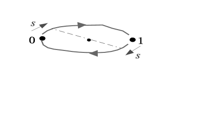
Figure 2: Cayley graph of the group ${\mathbb{Z}}_{2}=\{0,1\}$, represented as ${\mathcal{G}}=\{{\mathbb{I}},\sigma_{x}\}$ on ${\mathbb{C}}^{2}$. Points along the path which are specularly located relative to the center of the graph are correlated from the point of view of the averaging process. The parameter $s\in[0,\Delta t)$ measures the elapsed time within each subinterval.

On the graph pictured in figure 2, an Eulerian cycle ${\mathcal{P}_{E}}$ is described by the sequence of edges ${\mathcal{P}_{E}}=(\gamma,\gamma)$. Because the path determines the sequence of control Hamiltonians to be turned on along the cycle, in this case one simply obtains a control propagator given by

$$U_{c}(t)=\left\{\begin{array}[]{ll}u_{x}(t)&t\in[0,\Delta t)\\ u_{x}(s)\sigma_{x}&t\in[\Delta t,\Delta t+s)\>,\>s\in[0,\Delta t)\>.\end{array}\right.$$ (12)

By inserting the above expression in Eq. (7), the net phase evolution over a cycle becomes

$$\overline{\sigma_{z}}^{\,(E)} = \frac{1}{2\Delta t}\Big{(}\int_{0}^{\Delta t}ds\,u_{x}^{\dagger}(s)\sigma_{z}u_{x}(s)+\int_{0}^{\Delta t}ds\,{\sigma_{x}}u_{x}^{\dagger}(s)\sigma_{z}u_{x}(s){\sigma_{x}}\Big{)}$$ (13)

$$= \frac{1}{2\Delta t}\Big{(}\int_{0}^{\Delta t}ds\,u_{x}^{\dagger}(s)\sigma_{z}u_{x}(s)+\int_{0}^{\Delta t}ds\,u_{x}^{\dagger}(s)(\sigma_{x}\sigma_{z}\sigma_{x})u_{x}(s)\Big{)}$$

$$= \frac{1}{2\Delta t}\int_{0}^{\Delta t}ds\Big{(}u_{x}^{\dagger}(s)\sigma_{z}u_{x}(s)-u_{x}^{\dagger}(s)\sigma_{z}u_{x}(s)\Big{)}=0\>.$$

By comparing Eq. (13) with Eq. (10), one sees that the Eulerian protocol still achieves averaging by inducing an effective time reversal in the second control subinterval; however, such a reversal is now local in time, the evolution in the second interval continuously undoing the one in the first owing to the cancellations from opposite points in the graph (see figure 2).

The generalization of the above procedure to generic decoupling protocols is described in [26]. Under mild assumptions on the relevent control Hamiltonians, one can always ensure that the same ${\mathcal{G}}$-symmetri- zation of the BB limit is retained. However, Eulerian design turns out to be superior in two important respects: not only can any desired decoupling protocol be fully implemented using bounded-strength Hamiltonians, but the resulting schemes are also intrinsically stable against a large class of systematic control errors, thereby leading to enhanced robustness.

5 Relaxing timescale requirements: Decoupling of low-frequency noise

Going back to reconsidering decoupling timescale requirements, it turns out that they can be substantially weakened for a wide class of environments generating low-frequency noise. I will focus here on the most notable representative instance, provided by noise processes exhibiting a 1/$f$ spectrum. Noise phenomena consistent with a 1/$f$ behavior have been identified to play a role in an astonishing variety of dynamical systems, ranging from physics to biology, economics, and more. At the quantum level, 1/$f$ noise due to a variety of material-specific fluctuation mechanisms is ubiquitous in solid-state devices, with a severe impact on the performance of both nanoelectronic circuits [37] and qubit realizations. In particular, 1/$f$ noise due to fluctuating background charges is currently regarded as one of the primary decoherence sources for superconducting charge qubits [38].

An appropriate schematization of 1/$f$ noise effects requires going beyond the notion of a continuum of weakly coupled environmental modes at equilibrium which is embodied by standard harmonic-oscillator reservoirs. A quantum-mechanical model capturing the distinctive features of a realistic discrete environments generating 1/$f$ noise was recently investigated in [39]. Within a semiclassical approach that will suffice to the present discussion, a simple picture of 1/$f$ noise may be obtained by considering an incoherent superposition of relaxation processes from an ensemble of $M$ independent bistable fluctuators. Let $\xi_{k}(t)$ denote a random telegraph noise (RTN) signal describing the switching of an individual fluctuator between two values $\pm v_{k}/2$ with a total switching rate $\gamma_{k}$, and a corresponding Lorentzian power spectrum $S_{k}(\omega)=\gamma_{k}/(\gamma_{k}^{2}+\omega^{2})$, $\omega\in{\mathbb{R}}$. Provided that the switching rates in the ensemble are assumed to be distributed in a range $[\gamma_{min},\gamma_{max}]$ with probability

$${\mathbb{P}}(\gamma)=\frac{\text{const}}{\gamma}\,,\hskip 8.53581pt\text{const}=[\ln(\gamma_{max}/\gamma_{min})]^{-1}\>,$$ (14)

the total fluctuation $\Xi(t)=\sum_{k}\xi_{k}(t)$ exhibits a power spectrum $S(\omega)=\sum_{k}S_{k}(\omega)=A/|\omega|$, $A>0$, in a frequency interval $\gamma_{min}\ll\omega\ll\gamma_{max}$. For distributions of coupling strengths $\{v_{k}\}$ sufficiently peaked around their mean value $\langle v\rangle$, the parameter $A$ is directly related to the product $N_{d}\langle v\rangle^{2}$, $n_{d}=M/\log(\gamma_{max}/\gamma_{min})$ being the number of fluctuators per noise decade.

The simplest scenario for decoupling of 1/$f$ noise is obtained by considering a single qubit in the presence of the semiclassical RTN disturbance. Thus, the target system is described by a time-dependent effective Hamiltonian of the form

$$H_{0}(t)=H_{Q}+H_{RTN}(t)=[\Omega\sigma_{z}+\Delta\sigma_{x}]+\Xi(t)\sigma_{z}\>,$$ (15)

for real parameters $\Omega,\Delta$. While an appropriate extension of the basic average Hamiltonian formalism is needed in general to handle time-dependent target dynamics, the required control action can be implemented in this case through the same CP-protocol discussed for the spin-boson example of Section 3.1, either in the BB limit or in the Eulerian form illustrated in the previous section. A more detailed analysis of this problem is available in [40] (see also [41, 42, 43, 44] for related work). In what follows I only focus on some illustrative results in the pure dephasing limit, $\Delta=0$. In this regime, the stroboscopic evolution of the qubit coherence element may be exactly evaluated,

$$|\rho_{01}(t=NT_{c})|=\exp(-\Gamma_{c}(t))\,|\rho_{01}(t=0)|\>,$$ (16)

the analytic expression of the controlled decoherence functional being given in [40]. A formal result similar to Eq. (5) can be explicitly established in the continuous limit where $T_{c}\rightarrow 0,N\rightarrow\infty$. Thus, complete compensation of 1/$f$ effects requires access to control timescales $\Delta t\leq 1/\gamma_{max}$, so as to average out the influence of the fastest fluctuator present in the ensemble – as expected on general control-theoretic grounds. However, substantially slower decoupling rates might turn out to suffice in this case provided that the requirement of perfect suppression is lifted.

\psfrag{x}{$$ {\small time $(1/\Omega)$}}\psfrag{y}{${\text{e}^{-\Gamma_{c}(t)}}$}\includegraphics[width=209.58255pt,height=238.49121pt]{PQE-04-2figure3.eps}

Figure 3: Suppression of 1/$f$ pure dephasing, $\Omega=1,\Delta=0$, starting from the initial qubit state $|\psi\rangle=(|0\rangle+|1\rangle)/\sqrt{2}$. Solid lines: free evolution. For controlled evolutions, stroboscopic data (circles and diamonds) are connected by eye-guiding lines. In all cases, $\gamma_{max}=100$. From top to bottom, the other spectral parameters are as follows: (a) $\gamma_{min}=10^{-4}$, $\langle v\rangle=10^{-4}$; (b) $\gamma_{min}=10^{-6}$, $\langle v\rangle=10^{-4}$; (c) $\gamma_{min}=10^{-4}$, $\langle v\rangle=10^{-2}$. Control parameters are: (a) and (b) $\Delta t=1000$ (dot dashed), $\Delta t=100$ (dashed), $\Delta t=10$ (dotted); (c) $\Delta t=10$ (dot dashed), $\Delta t=1$ (dashed), $\Delta t=0.1$ (dotted).

The situation is pictorially summarized in figure 3. The three spectra differ due to the more or less pronounced Gaussian character of the underlying fluctuations, purely Gaussian dephasing (top plot) being closest to a formal representation in terms of a standard oscillator bath. As evidenced from the data, a $60\%$ coherence recovery is always achieved by $\Delta t$ values which are at least three orders of magnitude longer than expected from the inverse upper cutoff, the latter figure improving to five orders of magnitude for slower dephasing processes as in the top and middle panels. While such a favorable scaling in terms of decoupling resources might seem in a sense to naturally follow from the predominance of low-frequency modes in the noise profile, it is worth stressing that similar conclusions are not immediately applicable to the full class of possible 1/$f$ dynamics, the actual decoupling performance being in practice fairly sensitive to both the presence of strongly non-Gaussian noise sources and the operating point of the qubit [40]. Yet, this example convincingly shows the existence of realistic decoherence scenarios where decoupling might be achievable under affordable control resources.

6 Conclusions

Dynamical decoupling techniques offer a well-defined conceptual framework for addressing a variety of open-loop coherent-control problems for quantum systems. While their use as a tool for decoherence control is particularly relevant, the applicability of decoupling methods and concepts extends to a broader setting, encompassing schemes for quantum-dynamical engineering on both physical and encoded degrees of freedom [23].

From a practical standpoint, the implementation of decoupling schemes poses stringent requirements on the needed control operations. Although these are still beyond the reach of current experimental capabilities for many systems, progress in ultrafast coherent control is steady [45], hopefully making decoupling implementations less demanding for such systems in a near future. On the theoretical front, both the notion of Eulerian control and the decoupling of 1/$f$ noise indicate how conclusions based on the simplest decoupling protocols or on general control-theoretic bounds may be overly pessimistic, and that significant improvement may still be possible in relevant situations. It is my expectation that the convergence of better theoretical modeling and analysis, together with practical advances in quantum technologies, will improve the prospects that dynamical decoupling eventually becomes a method of choice for decoherence control.

References

- [1] Breuer, H.-P., and Petruccione, F., 2002, The Theory of Open Quantum Systems (New York: Oxford University Press).
- [2] Irreversible Quantum Dynamics, 2003, Benatti, F., and Floreanini, R., Eds. (Heidelberg: Springer-Verlag).
- [3] Nielsen, M. A., and Chuang, I. L., 2000, Quantum Computation and Quantum Information (Cambridge: Cambridge University Press).
- [4] See, for instance, Special Focus Issue on Experimental Proposals for Quantum Computation, 2000, Fortschr. Phys., 48, Number 9-11.
- [5] See Brumer, P. W., and Shapiro, M., 2003, Principles of the Quantum Control of Molecular Processes (New York: Wiley & Sons) for a general account. An experiment closely approaching quantum-limited sensitivity in a nanomechanical resonator was recently reported in LaHaye, M. D., Buu, O., Camarota, B., and Schwab, K. C., 2004, Science, 304, 74.
- [6] Lloyd, S., and Viola, L., 2002, Phys. Rev. A, 65, 010101, and references therein.
- [7] Altafini, C., 2003, J. Math. Phys., 44, 2357.
- [8] Poyatos, J. F., Cirac, J. I., and Zoller, P., 1996, Phys. Rev. Lett., 77, 4728.
- [9] Zanardi, P., and Rasetti, M., 1997, Phys. Rev. Lett., 79, 3306; Lidar, D. A., Chuang, I. L., and Whaley, K. B., 1998, ibid., 81, 2594.
- [10] Knill, E., Laflamme, R., and Viola, L., 2000, Phys. Rev. Lett., 84, 2525.
- [11] Kitaev, A., 2003, Ann. Phys., 303, 2; Bravy, S., and Kitaev, A., 1998, quant-ph/9811052.
- [12] Zanardi, P., and Lloyd, S., 2003, Phys. Rev. Lett., 90, 067902.
- [13] Wiseman, H. M., 1994, Phys. Rev. A, 49, 2133; ibid., 50, 4428. See also Ahn, C., Wiseman, H. M., and Milburn, G. J., 2003, Phys. Rev. A, 67, 052310.
- [14] Shor, P. W., 1995, Phys. Rev. A, 52, 2493.
- [15] Steane, A. M., 1996, Phys. Rev. Lett., 77, 793.
- [16] Viola, L., and Lloyd, S., 1998, Phys. Rev. A, 58, 2733.
- [17] Viola, L., Knill, E., and Lloyd, S., 1999, Phys. Rev. Lett., 82, 2417.
- [18] Hahn, E. L., 1950, Phys. Rev., 80, 580.
- [19] Haeberlen, U., and Waugh, J. S., 1968, Phys. Rev., 175, 453.
- [20] Viola, L., Lloyd, S., and Knill, E., 1999, Phys. Rev. Lett., 83, 4888.
- [21] Zanardi, P., 1999, Phys. Lett. A, 258, 77.
- [22] Vitali, D., and Tombesi, P., 1999, Phys. Rev. A, 59, 4178.
- [23] Viola, L., 2002, Phys. Rev. A, 66, 012307, and references therein.
- [24] Lidar, D. A., and Wu, W.-A., 2002, Phys. Rev. Lett., 88, 017905; Wu, W.-A., and Lidar, D. A., 2002, ibid., 207902.
- [25] Byrd, M. S., and Lidar, D. A., 2002, Quantum Inf. Proc., 1, 19.
- [26] Viola, L., and Knill, E., 2003, Phys. Rev. Lett., 90, 037901.
- [27] See, for instance, Wocjan, P., Rötteler, M., Janzing, D., and Beth, Th., 2002, Quantum Inf. Comput., 2, 133; Bennett, C. H., et al., 2002, Phys. Rev. A, 66, 012305.
- [28] Ernst, R. R., Bodenhausen, G., and Wokaun, A., 1994, Principles of Nuclear Magnetic Resonance in One and Two Dimensions (Oxford: Oxford University Press).
- [29] Gheorghiu-Svirchevski, S., 2002, Phys. Rev. A, 66, 032101.
- [30] Uchiyama, C., and Aihara, M., 2002, Phys. Rev. A, 66, 032313.
- [31] Berglund, A. J., 2000, quant-ph/0010001.
- [32] Search, C., and Berman, P. R., 2000, Phys. Rev. Lett., 85, 2272.
- [33] Agarwal, G. S., Scully, M. O., and Walther, W., 2001, Phys. Rev. Lett., 86, 4271.
- [34] Scully, M. O., and Zubairy, M. S., 2001, Phys. Rev. A, 64, 022304.
- [35] Viola, L., Knill, E., and Lloyd, S., 2000, Phys. Rev. Lett., 85, 3520.
- [36] Bollobás, B., 1998, Modern Graph Theory (New York: Sprin- ger-Verlag).
- [37] Peters, M. G., Dijkhuis, J. I., and Molenkamp, L. W., 1999, J. Appl. Phys., 86, 1523; Collins, P. G., Fuhrer, M. S., and Zettl, A., 2000, ibid., 76, 894; Covington, M., Keller, M. W., Kautza, R. L., and Martinis, J., 2000, Phys. Rev. Lett., 84, 5192.
- [38] Nakamura, Y., Pashkin, Yu. A., Yamamoto, T., and Tsai, J. S., 2002, Phys. Rev. Lett., 88, 047901; 2002, Phys. Scripta, 102, 155.
- [39] Paladino, E., Faoro, L., Falci, G., and Fazio, R., 2002, Phys. Rev. Lett., 88, 228304.
- [40] Faoro, L., and Viola, L., 2004, Phys. Rev. Lett., 92, 117905.
- [41] Shiokawa, K., and Lidar, D. A., 2004, Phys. Rev. A, 69, 030302.
- [42] Gutmann, H., Wilhelm, F. K., Kaminsky, W. M., and Lloyd, S., 2003, cond-mat/0308107.
- [43] Falci, G., D’Arrigo, A., Mastellone, A., and Paladino, E., 2003, cond-mat/0312442.
- [44] Galperin, Y. M., Altshuler, B. L., and Shantsev, D. V., 2003, cond-mat/0312490.
- [45] See, for instance, Bucksbaum, P. H., 2003, Nature, 421, 593 for a recent highlight.