Intrinsic Entanglement Degradation by Multi-Mode Detection

Abstract

Relations between photon scattering, entanglement and multi-mode detection are investigated. We first establish a general framework in which one- and two-photon elastic scattering processes can be discussed, then we focus on the study of the intrinsic entanglement degradation caused by a multi-mode detection. We show that any multi-mode scattered state cannot maximally violate the Bell-CHSH inequality because of the momentum spread. The results presented here have general validity and can be applied to both deterministic and random scattering processes.

I Introduction

During the last fifteen years, the concept of entanglement has passed from the inhospitable realm of the “problems in the foundation of quantum mechanics” Ballentine (1986), to the fashionable fields of quantum information and computation Nielsen and Chuang (2002). Experimental availability Zeilinger (1999) of reliable sources of entangled quantum bits (qubits) in the optical domain has been one of the major boosts for this rapid transition. Polarization-entangled photon pairs produced in a spontaneous parametric down conversion (SPDC) process Yariv (1989) have thus become an essential tool in experimental quantum information science Gisin et al. (2002).

Robustness of photon polarization-entanglement is important when propagation over long distances of entangled states is required. However, during propagation in a medium photons may be depolarized by scattering processes due to imperfections. Further, the recently observed transfer of quantum entanglement from photons to a linear medium and back to photons Altewischer et al. (2002), has also been described as an elastic scattering process Sca . In general, polarization-dependent scattering may affect more or less the entanglement of a photon pair depending on the properties of the scattering medium Vel ; Woe .

In this paper we show that independently from the details of the scattering process, the polarization entanglement of a photon pair is unavoidably degraded by a multi-mode measurement Woe . Moreover, we show that, contrary to common belief, it is not always possible to build a $2\times 2$ reduced density matrix (or $4\times 4$ in the case of entangled pairs) to describe the scattered state. This fact was recently recognized by Peres and coworkers Per for the case of a single polarization qubit, as opposed to the case of two-photon entangled qubits considered here. They circumvented this difficulty by introducing, at a certain stage of their calculations, the unphysical concept of longitudinal photons. In this way they were able to build a $3\times 3$ effective reduced density matrix whose physical content can be obtained from a family of positive operator-valued measures (POVMs Peres (1998)).

In this paper we follow a somewhat different approach. We show that the difficulties one encounters in trying to define a reduced density matrix, are also due to the troubling determination of the effective dimension of the Hilbert space in which the two-photon entangled state can be represented. In fact, due to the transverse nature of the free electromagnetic field, in a multi-mode scattering process the momentum and the polarization degrees of freedom become entangled. Therefore, after the scattering, the two-photon polarization-entangled state is no longer confined to a $4$-dimensional Hilbert space, but spans an higher-dimensionality space. We show that under certain circumstances this dimension may remain bigger than $4$ even after tracing out the momentum degrees of freedom. In this case a traditional Bell-violation measurement setup may fail to reveal a maximal violation of the Bell-CHSH inequality. However, the detailed investigation of the entanglement properties of this kind of high-dimensional scattered photon-pair Collins et al. (2002); Law et al. (2000); Law and Eberly (2004), is left to a forthcoming paper Aie .

This paper is structured as follows. In Sec. II we define the general framework for the discussion of one- and two-photon scattering processes. In Sec. III, starting from an experimentalist point of view, we adopt an operational way to define the photon polarization states in terms of the physically detected states. Furthermore, we calculate the classical Jones matrix Kliger et al. (1990) corresponding to an arbitrarily oriented polarizer and use it to introduce a suitable field creation operator to build explicitly the physical photon states. In this way we can introduce a $2\times 2$ effective density matrix by a projection operation on the one-photon physical states. The concept of effective density matrix is extended to polarization-entangled photon-pair states, in the first part of Sec. IV. Then, in the second part of Sec. IV we quantify the entanglement degradation by calculating the effect of a polarization detection mismatch on the mean value $\langle\mathcal{B}_{\mathrm{CHSH}}\rangle$ of the Bell-CHSH operator Braunstein et al. (1992) for the set of the Schmidt states Aravind (1995). Finally, we summarize our main conclusions in Sec. V.

II One-Photon Scattering

II.1 One-photon states and their representation

To understand the effects that a scattering process may have on a single photon wave packet, we start by introducing a proper notation. Let ${\mathbf{A}}(\mathbf{r},t)$ denote the transverse part of the electromagnetic potential. In the Coulomb gauge the quantization procedure can be carried out straightforwardly Lee (1988) to obtain the corresponding field operators $\hat{\mathcal{A}}(\mathbf{r},t)$. At any given time $t$, $\hat{\mathcal{A}}(\mathbf{r},t)$ may be expanded in terms of the Fourier series

$$\hat{\mathcal{A}}(\mathbf{r},t)=\sum_{\mathbf{k}}\frac{1}{\sqrt{2\omega\Omega}}\left[\hat{\mathbf{a}}_{\mathbf{k}}(t)e^{i\mathbf{k}\cdot\mathbf{r}}+\mathrm{h.c.}\right],$$ (1)

where $\omega=|\mathbf{k}|$, $\hat{\mathbf{a}}_{\mathbf{k}}(t)\cdot\mathbf{k}=0$, and natural units $(c=\hbar=1)$ have been used. With $\Omega$ we denote the quantization volume. For any given $\mathbf{k}$ we may define a set of three real orthogonal unit vectors $\hat{\mathbf{k}}\equiv\mathbf{k}/|\mathbf{k}|$, $\hat{\mathbf{e}}_{\mathbf{k}}^{(1)}$, $\hat{\mathbf{e}}_{\mathbf{k}}^{(2)}$ such that

$$\hat{\mathbf{e}}_{\mathbf{k}}^{(1)}\cdot\hat{\mathbf{e}}_{\mathbf{k}}^{(2)}=0,\qquad\hat{\mathbf{e}}_{\mathbf{k}}^{(1)}\times\hat{\mathbf{e}}_{\mathbf{k}}^{(2)}=\hat{\mathbf{k}}.$$ (2)

It is convenient to introduce the creation operators $\hat{a}^{\dagger}_{\mathbf{k}s}$ of a photon with momentum $\mathbf{k}$ and helicity $s=\pm 1$ as

$$\hat{a}^{\dagger}_{\mathbf{k}s}=\hat{\mathbf{a}}^{\dagger}_{\mathbf{k}}\cdot\hat{\mathbf{f}}_{\mathbf{k}}^{(s)},$$ (3)

where the complex vectors $\hat{\mathbf{f}}_{\mathbf{k}}^{(s)}$ are defined as

$$\hat{\mathbf{f}}_{\mathbf{k}}^{(s)}=\frac{1}{\sqrt{2}}\left(\hat{\mathbf{e}}_{\mathbf{k}}^{(1)}+is\,\hat{\mathbf{e}}_{\mathbf{k}}^{(2)}\right),\qquad(s=\pm 1).$$ (4)

They satisfy the canonical commutation rules

$$\left[\hat{a}_{\mathbf{k}s}(t),\hat{a}^{\dagger}_{\mathbf{k}^{\prime}s^{\prime}}(t)\right]=\delta_{\mathbf{k}\mathbf{k}^{\prime}}\delta_{ss^{\prime}}.$$ (5)

Then, an one-photon helicity basis state can be written as

$$|\mathbf{k},s(\mathbf{k})\rangle\equiv\hat{a}^{\dagger}_{\mathbf{k}s}|0\rangle,$$ (6)

where $|0\rangle$ denotes the vacuum state of the free electromagnetic field. This state represents a photon with momentum $\mathbf{k}$ and helicity $s(\mathbf{k})=\pm 1$, that is $|\mathbf{k},s(\mathbf{k})\rangle$ is an eigenstate of the momentum operator $\hat{\mathbf{K}}\equiv\sum_{\mathbf{k}^{\prime},s^{\prime}}\mathbf{k}^{\prime}\hat{a}^{\dagger}_{\mathbf{k}^{\prime}s^{\prime}}\hat{a}_{\mathbf{k}^{\prime}s^{\prime}}$ with eigenvalue $\mathbf{k}$:

$$\hat{\mathbf{K}}|\mathbf{k},s(\mathbf{k})\rangle=\mathbf{k}|\mathbf{k},s(\mathbf{k})\rangle.$$ (7)

Because of Eq. (7), the one-photon-space basis states $|\mathbf{k},s(\mathbf{k})\rangle$ are often said to be the direct products of momentum and polarization states and this is usually stated by writing

$$|\mathbf{k},s(\mathbf{k})\rangle\equiv|\mathbf{k}\rangle\otimes|s(\mathbf{k})\rangle.$$ (8)

However, one should realize that the left side of this equation is a genuine QED state, while the right side is just one of its possible representations. To be more specifics in QED there is no such a thing like a momentum creation operator that creates from the vacuum a momentum state $|\mathbf{k}\rangle$, nor is there a polarization creation operator which create a polarization state $|s(\mathbf{k})\rangle$. Nevertheless the “momentum $\otimes$ polarization” representation for the one-photon states has several advantages. For this reason we now present formally a few elementary facts about this representation.

II.1.1 Some elementary facts

Let us consider two one-photon states $|\psi_{\mathbf{k}}\rangle$ and $|\phi_{\mathbf{q}}\rangle$ which are eigenstates of the momentum operator with eigenvalues $\mathbf{k}$ and $\mathbf{q}$ respectively:

$$\begin{array}[]{rcl}|\psi_{\mathbf{k}}\rangle&=&\psi_{+}(\mathbf{k})|\mathbf{k},1\rangle+\psi_{-}(\mathbf{k})|\mathbf{k},-1\rangle,\\ \\ |\phi_{\mathbf{q}}\rangle&=&\phi_{+}(\mathbf{q})|\mathbf{q},1\rangle+\phi_{-}(\mathbf{q})|\mathbf{q},-1\rangle.\end{array}$$ (9)

They can be represented as

$$|\psi_{\mathbf{k}}\rangle\doteq\left(\begin{array}[]{c}\psi_{+}\\ \psi_{-}\end{array}\right)_{\mathbf{k}},\qquad|\phi_{\mathbf{q}}\rangle\doteq\left(\begin{array}[]{c}\phi_{+}\\ \phi_{-}\end{array}\right)_{\mathbf{q}},$$ (10)

where the symbol “$\doteq$” stands for “is represented by”, and we have used the subscripts $\mathbf{k}$ and $\mathbf{q}$ for the representations of $|\psi_{\mathbf{k}}\rangle$ and $|\phi_{\mathbf{q}}\rangle$ respectively, to stress the fact that they belong to different vector spaces. Since

$$\left(\begin{array}[]{c}\psi_{+}\\ \psi_{-}\end{array}\right)_{\mathbf{k}}=\psi_{+}\left(\begin{array}[]{c}1\\ 0\end{array}\right)_{\mathbf{k}}+\psi_{-}\left(\begin{array}[]{c}0\\ 1\end{array}\right)_{\mathbf{k}},$$ (11)

we can write

$$|\psi_{\mathbf{k}}\rangle\doteq\psi_{+}|+)_{\mathbf{k}}+\psi_{-}|-)_{\mathbf{k}},$$ (12)

where we have defined

$$|+)_{\mathbf{k}}\doteq\left(\begin{array}[]{c}1\\ 0\end{array}\right)_{\mathbf{k}},\qquad|-)_{\mathbf{k}}\doteq\left(\begin{array}[]{c}0\\ 1\end{array}\right)_{\mathbf{k}}.$$ (13)

In the equations above we have used the parenthesis symbols $|\pm)_{\mathbf{k}}$ for the basis vectors instead of the usual bracket $|\cdot\rangle$ ones to underline the fact that they are not genuine QED states, that is they are not created from the vacuum by any bosonic creation operator. Then, from now on, we shall reserve the bracket symbols $|\cdot\rangle$ only for the truly QED states.

The two vectors displayed in Eq. (13) form a basis $\mathcal{B}_{\mathbf{k}}$ for a two-dimensional “polarization” space $\mathcal{H}_{\mathbf{k}}$. Exactly in the same way we can introduce a basis $\mathcal{B}_{\mathbf{q}}=\{|+)_{\mathbf{q}},|-)_{\mathbf{q}}\}$ for the space $\mathcal{H}_{\mathbf{q}}$ relative to the (arbitrary) momentum $\mathbf{q}$. More generally, let $K$ be a $N$-dimensional set of momenta: $K=\{\mathbf{k}_{1},\ldots,\mathbf{k}_{N}\}$. Then we can build a $2N$-dimensional space $\mathcal{H}$ spanned by the basis $\mathcal{B}=\mathcal{B}_{\mathbf{k}_{1}}\cup\dots\cup\mathcal{B}_{\mathbf{k}_{N}}$ as

$$\mathcal{H}=\mathcal{H}_{\mathbf{k}_{1}}\oplus\dots\oplus\mathcal{H}_{\mathbf{k}_{N}}.$$ (14)

It is clearly possible to introduce other bases in $\mathcal{H}$. For example let $\{|\mathbf{k}_{i})\}$, ($i=1,\ldots,N$) and $\{|+),|-)\}$ be a $N$-dimensional and a $2$-dimensional sets of basis vectors respectively, represented by

$$|\mathbf{k}_{i})\doteq\left(\begin{array}[]{c}0\\ \vdots\\ 1\\ \vdots\\ 0\end{array}\right),\quad|+)\doteq\left(\begin{array}[]{c}1\\ 0\end{array}\right),\quad|-)\doteq\left(\begin{array}[]{c}0\\ 1\end{array}\right).$$ (15)

where all elements of $|\mathbf{k}_{i})$ are zero with the exception of element $i$ which is equal to $1$. Then the set given by the vectors

$$|\mathbf{k}_{i})\otimes|s)\equiv|\mathbf{k}_{i},s),\qquad\left(\begin{array}[]{c}i=1,\ldots,N,\\ s=\pm 1,\end{array}\right)$$ (16)

is an orthonormal and complete basis of $\mathcal{H}$. Now, the factorization “momentum $\otimes$ polarization” in Eq. (16) is absolutely legitimate without introducing any “ad hoc” creation operator. We would like to stress once again the fact that the genuine QED states $|\mathbf{k},s(\mathbf{k})\rangle$ are not factored, just their representation $|\mathbf{k},s)$. Moreover, the helicity label $s$ in Eq. (16) does not depend on the momentum $\mathbf{k}$, so it is not longer a secondary variable Per . Note that we have chosen to work with the helicity eigenstates $|\mathbf{k},s(\mathbf{k})\rangle$ but we could have worked equally well with the linear polarization basis vectors $|\mathbf{k},\alpha(\mathbf{k})\rangle$, where $\alpha=x,y$.

II.1.2 Tracing over the momenta

The reason for which we have introduced the factorizable basis vectors $|\mathbf{k},s)$ in the previous subsection, is that we want to be able to separate the momentum degrees of freedom from the polarization ones. This separation becomes important when the photons are subjected to polarization tests only, and the momenta become irrelevant degrees of freedom. Then, it is a standard practice Peres (1998) to introduce a reduced density matrix obtained from the complete one, by tracing over some subset of the whole set of the field momenta.

Let $\hat{\rho}$ be the density matrix describing the state of a single photon. We can represent $\hat{\rho}$ in $\mathcal{H}$ by defining the $N^{2}$ matrices $R(n,m)$ ($2\times 2$) whose elements are calculated with the usual QED rules:

$${R}_{ss^{\prime}}(n,m)\equiv Z_{1}\langle\mathbf{k}_{n},s(\mathbf{k}_{n})|\hat{\rho}|\mathbf{k}_{m},s^{\prime}(\mathbf{k}_{m})\rangle,$$ (17)

where $Z_{1}$ is an arbitrary normalization constant and $(s,s^{\prime}=\pm 1)$. These matrices are the building blocks of the total representation of $\hat{\rho}$:

$$\hat{\rho}\doteq\left(\begin{array}[]{ccc}\left[\begin{array}[]{cc}R_{++}(1,1)&R_{+-}(1,1)\\ R_{-+}(1,1)&R_{--}(1,1)\end{array}\right]&\dots&R(1,N)\\ \vdots&\ddots&\vdots\\ R(N,1)&\dots&R(N,N)\end{array}\right).$$ (18)

From now on, we choose $Z_{1}$ such that $\mathrm{Tr}\hat{\rho}=1$. Now, if we want to calculate the reduced density matrix $\hat{\rho}^{\mathrm{R}}_{1}$, obtained by tracing out the momentum degrees of freedom, what we have to do is simply to take all the diagonal blocks $R(n,n)$ and sum them together:

$$\hat{\rho}^{\mathrm{R}}_{1}\doteq\sum_{n=1}^{N}R(n,n)\equiv\rho^{\mathrm{R}}_{1}.$$ (19)

The matrix $\rho^{\mathrm{R}}_{1}$ is a well defined $2\times 2$ matrix and there is no ambiguity in its determination. We have used the subscript $1$ in writing $\rho^{\mathrm{R}}_{1}$ to distinguish it from the generalized reduced density matrix $\rho^{\mathrm{R}}$ we shall introduce in the next subsection. However, it was recently shown that a reduced density matrix introduced as above, has no meaning because it does not have definite transformation properties Lin . Besides this fact, there are more practical reasons for which $\rho^{\mathrm{R}}_{1}$ (at least a single one) cannot be introduced, as we shall see in the next subsection. For the moment let us see very shortly how the traditional approach works and why it may fail. If one deals with operators that are factorizable in the basis $\{|\mathbf{k}_{i},s)\}$, that is if they can be represented as

$$\hat{X}\doteq|X)(X|\otimes\sum_{n=1}^{N}|\mathbf{k}_{n})(\mathbf{k}_{n}|,$$ (20)

where the right side of this equation is, in fact, the direct product of a $2\times 2$ matrix (polarization part, momentum independent), times a $N\times N$ matrix (momentum part, polarization independent). Then the average value $\langle\hat{X}\rangle=\mathrm{Tr}(\hat{\rho}\hat{X})$ can be certainly written as

$$\bigl{\langle}\hat{X}\bigr{\rangle}=\mathrm{Tr}\bigl{(}\hat{\rho}^{\mathrm{R}}_{1}|X)(X|\bigr{)},$$ (21)

and, apparently, there are no problems in using $\hat{\rho}^{\mathrm{R}}_{1}$. The key point here, is that the operator representation with respect to the factorizable basis $\{|\mathbf{k}_{n},s)\}$ may have no meaning at all because the polarization state $|X)$ in Eq. (20) does not depend on $\mathbf{k}$ while the polarization state of a photon is always referred to a given momentum, as shown in Eq. (3). Then, in a multi-mode process where many values of the photon momentum are involved, it becomes impossible to define a unique $2\times 2$ reduced density matrix ($|X)(X|$ in Eq. (20)), instead one must deal with a different matrix for each different momentum. This will be explicitly shown in the next subsection.

II.2 One-Photon Scattering

Let us consider now a one-photon state approximatively represented by the monochromatic plane wave $|\mathbf{k}_{0},s_{0}(\mathbf{k}_{0})\rangle_{\mathrm{in}}$, and suppose that it is elastically scattered by a certain medium. The final state $|\psi_{f}\rangle$ of the photon after the scattering process can be written in terms of the output states $|\mathbf{k},s(\mathbf{k})\rangle$ as

$$|\psi_{f}\rangle=\sum_{\mathbf{k}\in K}\sum_{s=\pm 1}\psi_{s}(\mathbf{k})|\mathbf{k},s(\mathbf{k})\rangle,$$ (22)

where $\psi_{s}(\mathbf{k})\equiv\langle\mathbf{k},s(\mathbf{k})|\mathbf{k}_{0},s_{0}(\mathbf{k}_{0})\rangle_{\mathrm{in}}$ represent the probability amplitude that the photon is scattered in a state with momentum $\mathbf{k}$ and helicity $s(\mathbf{k})$, where $|\mathbf{k}|\cong\omega_{0}$. With $K$ we have denoted the set of all scattered modes. By inspecting Eq. (22) one immediately realizes that in the scattered state $|\psi_{f}\rangle$ the polarization and momentum degrees of freedom are entangled because the helicity states $|s(\mathbf{k})\rangle$ depend explicitly from $\mathbf{k}$ and the two sums are not independent. In other words, in general, $|\psi_{f}\rangle$ is not an eigenstate of the linear momentum operator $\hat{\mathbf{K}}$.

Now suppose that we measure some polarization property of the scattered photon, regardless of its momentum. To be more specific let us assume that a polarization analyzer (a dichroic sheet polarizer or a crystal prism polarizer) is present in a plane perpendicular to the wave-vector $\mathbf{k}_{0}$ of the impinging photon and that we collect, with a photo-detector, all the light coming from the scattering target within a certain angular aperture $\Theta_{D}$. With this experimental configuration we test only the photon polarization, irrespective of the plane-wave mode $\mathbf{k}$ where the photon is to be found within $\Theta_{D}$. We call this kind of experimental arrangement, a multi-mode detection scheme.

The act of measurement can be quantified by calculating, for example, the mean value of the operator $\hat{P}$ defined as:

$$\hat{P}=\sum_{\mathbf{k}\in K_{D}}\sum_{s,s^{\prime}}P_{ss^{\prime}}(\mathbf{k})|\mathbf{k},s(\mathbf{k})\rangle\langle\mathbf{k},s^{\prime}(\mathbf{k})|,$$ (23)

where

$$P(\mathbf{k})=\left(\begin{array}[]{cc}P_{++}(\mathbf{k})&P_{+-}(\mathbf{k})\\ P_{-+}(\mathbf{k})&P_{--}(\mathbf{k})\end{array}\right),$$ (24)

is a $2\times 2$ Hermitian matrix such that $P^{2}=P$ and $K_{D}$ is the set of the detected modes:

$$\{\mathbf{k}\in K_{D}|\,\left|\mathbf{k}\cdot\mathbf{k}_{0}\right|/\omega_{0}^{2}\lesssim|\cos\Theta_{D}|\}.$$

Moreover we assume, for definiteness, $\dim K_{D}=N$ and $K_{D}\subset K$. It is easy to see that $\hat{P}$ is a projector ($\hat{P}^{2}=\hat{P}$), and that it commutes with the momentum operator $\hat{\mathbf{K}}$:

$$\bigl{[}\hat{P},\hat{\mathbf{K}}\bigr{]}=\mathbf{0}.$$ (25)

It is also easy to understand that the equation above is the equivalent, in the QED context, of the factorizability condition expressed in Eq. (20). The matrix elements of $\hat{P}$ are

$$\begin{array}[]{rcl}P_{ss^{\prime}}(n,m)&\equiv&\langle\mathbf{k}_{n},s(\mathbf{k}_{n})|\hat{P}|\mathbf{k}_{m},s^{\prime}(\mathbf{k}_{m})\rangle\\ \\ &\equiv&P_{ss^{\prime}}(n)\delta_{nm}.\end{array}$$ (26)

From Eq. (26) is clear that $\hat{P}$ has a block-diagonal shape:

$$\hat{P}\doteq\left(\begin{array}[]{ccc}\left[\begin{array}[]{cc}P_{++}(1)&P_{+-}(1)\\ P_{-+}(1)&P_{--}(1)\end{array}\right]&&\\ &\ddots&\\ &&P(N)\end{array}\right),$$ (27)

so that only the corresponding diagonal blocks of $\hat{\rho}$ will enter in the calculation of $\langle\hat{P}\rangle$. Explicitly

$$\langle\hat{P}\rangle=\sum_{n=1}^{N}\mathrm{Tr}\bigl{(}R(n)P(n)\bigr{)},$$ (28)

where Eq. (18) has been used and $R(n)\equiv R(n,n)$ for short. Then, the form of the operator $\hat{P}$ in Eq. (27) naturally leads to the introduction of a generalized reduced density matrix ${\rho}^{\mathrm{R}}$ ($2N\times 2N$) defined as:

$${\rho}^{\mathrm{R}}=\mathrm{diag}\{R(1),\ldots,R(N)\}=\left(\begin{array}[]{ccc}R(1)&&\\ &\ddots&\\ &&R(N)\end{array}\right),$$ (29)

Thus, differently from Eq. (19) were we have found a unique $2\times 2$ matrix, we have now to deal with a set of $N$ different $2\times 2$ matrices $\{R(1),\ldots,R(N)\}$: one matrix $R(n)$ per each mode $\mathbf{k}_{n}$ of the field. This is due to the form of the operator $\hat{P}$. Only in the hypothetical case in which the matrix elements $P_{ss^{\prime}}(\mathbf{k})$ of $\hat{P}$ were independent from $\mathbf{k}$, we would obtain again a unique $2\times 2$ density matrix defined as $\rho^{\mathrm{R}}_{1}=\sum_{n=1}^{N}R(n)$.

What does all this mean? We can get some insights into the above equations, by rewriting them in the basis $\mathcal{B}=\mathcal{B}_{\mathbf{k}_{1}}\cup\dots\cup\mathcal{B}_{\mathbf{k}_{N}}$ introduced previously. Let us start by defining the normalized state $|\phi)_{\mathbf{k}}$ in the basis $\mathcal{B}_{\mathbf{k}}$ as

$$|\phi)_{\mathbf{k}}=\frac{1}{\sqrt{\zeta(\mathbf{k})}}\sum_{s=\pm 1}\psi_{s}(\mathbf{k})|s)_{\mathbf{k}},$$ (30)

where the complex amplitudes $\psi_{s}(\mathbf{k})$ are defined in Eq. (22) and

$$\zeta(\mathbf{k})\equiv|\psi_{+}(\mathbf{k})|^{2}+|\psi_{-}(\mathbf{k})|^{2}.$$ (31)

Then we can represent the one-photon state $|\psi_{f}\rangle$ in Eq. (22), restricted to $K_{D}$, as

$$|\psi_{f}\rangle\doteq\bigcup_{\mathbf{k}\in K_{D}}|\phi)_{\mathbf{k}}.$$ (32)

Then, by combining Eq. (17) with Eq. (22) we find

$$R_{ss^{\prime}}(n,m)=Z_{1}\psi_{s}(\mathbf{k}_{n})\psi_{s^{\prime}}^{*}(\mathbf{k}_{m}).$$ (33)

From the equation above and the normalization condition $\mathrm{Tr}R=1$, it follows that

$$Z_{1}=1/\sum_{\mathbf{k}\in K_{D}}\zeta(\mathbf{k}).$$ (34)

It should be clear now that if we define the pure-state density matrix $\hat{\rho}_{\phi}(\mathbf{k})$ as

$$\hat{\rho}_{\phi}(\mathbf{k})\equiv|\phi)_{\mathbf{k}}\,\/{}_{\mathbf{k}}\!(\phi|,$$ (35)

then we can write the generalized reduced density matrix $\hat{\rho}^{\mathrm{R}}$ as the direct sum, as opposed to the ordinary sum in Eq. (19), of all the sub-matrices $\hat{\rho}_{\phi}(\mathbf{k})$:

$$\begin{array}[]{rcl}\hat{\rho}^{\mathrm{R}}&=&\displaystyle{{\bigoplus_{\mathbf{k}\in K_{D}}}w(\mathbf{k})\hat{\rho}_{\phi}(\mathbf{k})}\\ \\ &=&\displaystyle{{\bigoplus_{\mathbf{k}\in K_{D}}}|\phi)_{\mathbf{k}}\,w(\mathbf{k})\,\/_{\mathbf{k}}\!(\phi|},\end{array}$$ (36)

were the statistical weight function $w(\mathbf{k})$ is equal to

$$w(\mathbf{k})=Z_{1}\zeta(\mathbf{k})=\frac{\zeta(\mathbf{k})}{\displaystyle{\sum_{\mathbf{k}^{\prime}\in K_{D}}\zeta(\mathbf{k}^{\prime})}},$$ (37)

and $\displaystyle{\sum_{\mathbf{k}\in K_{D}}}w(\mathbf{k})=1$. So we find that the price to pay for introducing a polarization basis $\mathcal{B}$, is that we have to deal with a generalized reduced density matrix which is expressed as a direct sum instead of an ordinary sum. Of course, this fact is entirely due to the incomplete nature of the polarization representation; there are no problems in writing $\hat{\rho}^{\mathrm{R}}$ as an ordinary sum in the QED formalism. In such a context we have to use the complete momentum eigenstate basis $\{|\mathbf{k},s(\mathbf{k})\rangle\}$ in order to write

$$\hat{\rho}^{\mathrm{R}}=\sum_{\mathbf{k}\in K_{D}}w(\mathbf{k})|\mathbf{k},\phi(\mathbf{k})\rangle\langle\mathbf{k},\phi(\mathbf{k})|,$$ (38)

where we have defined the momentum eigenstates $|\mathbf{k},\phi(\mathbf{k})\rangle$ as

$$|\mathbf{k},\phi(\mathbf{k})\rangle\equiv\frac{1}{\sqrt{\zeta(\mathbf{k})}}\sum_{s=\pm 1}\psi_{s}(\mathbf{k})|\mathbf{k},s(\mathbf{k})\rangle.$$ (39)

Not surprisingly, $\hat{\rho}^{\mathrm{R}}$ has the same “momentum-diagonal” structure as $\hat{P}$ in Eq. (23). It clearly represents a mixed state because $(\hat{\rho}^{\mathrm{R}})^{2}\neq\hat{\rho}^{\mathrm{R}}$. Eq. (38) can be interpreted by saying that from the observer point of view (who supposedly cannot measure the photon momentum), things go as if the scatterer were a thermal source emitting photons in the states $|\mathbf{k},s(\mathbf{k})\rangle$ with probabilities $w(\mathbf{k})$.

Thus, we have shown that it is impossible to extract from $\hat{\rho}^{\mathrm{R}}$ in a straightforward way a unique $2\times 2$ reduced density matrix; rather we have obtained a $N$-dimensional set $\{R(1),\dots,R(N)\}$ of $2\times 2$ matrices, each of them well defined in its proper Hilbert space specified by the momentum $\mathbf{k}$. This is a direct consequence of the fact that helicity of a photon can be defined only with respect to a given momentum Per . It is worth to note that this result is not in contrast with existence of a $4\times 4$ density matrix for two polarization-entangled photons emitted in a SPDC process. In fact, in that case, each photon is emitted in one mode of the electromagnetic field and the two-photon state is still an eigenstate of the total linear momentum. However, in Sec. III we shall introduce an effective reduced density matrix $\rho_{\mathrm{eff}}$ both for the one-photon and two-photon states.

In order to perform an actual calculation, we have to give a rule how to obtain the matrix elements $P_{ss^{\prime}}(\mathbf{k})$ in Eq. (23). From a physical point of view they can be expressed as suitable linear combinations of the probability amplitude that a photon with definite momentum $\mathbf{k}$ and linear polarization $\alpha(\mathbf{k})$, is transmitted across a linear polarizer with a given orientation $\hat{\mathbf{p}}$. The next Section will be devoted to the search of an explicit expression for $P_{ss^{\prime}}(\mathbf{k})$.

III Physical Polarization States

In this section we study how a single-photon state changes when the photon crosses an arbitrarily oriented polarizer. Then we use this information to build an effective reduced density matrix.

III.1 Classical Polarization States

A lossless linear polarizer Born and Wolf (1984) is a planar device which can be characterized by two orthogonal vectors: the axis $\hat{\mathbf{n}}$ and the orientation $\hat{\mathbf{p}}$. The first vector is orthogonal to the plane of the polarizer, while the second one lies in that plane: $\hat{\mathbf{p}}\cdot\hat{\mathbf{n}}=0$. From now on, with the sentence “a polarizer $(\hat{\mathbf{p}},\hat{\mathbf{n}})$” we shall indicate a linear polarizer with orientation $\hat{\mathbf{p}}$ and axis $\hat{\mathbf{n}}$.

For the moment we consider only classical fields, later we shall introduce the corresponding quantum operators. Following Mandel and Wolf Mandel and Wolf (1995), we consider a polarizer $(\hat{\mathbf{p}},\hat{\mathbf{z}})$ where $\hat{\mathbf{p}}=\hat{\mathbf{x}}\cos\beta+\hat{\mathbf{y}}\sin\beta$ and $\hat{\mathbf{x}},\hat{\mathbf{y}},\hat{\mathbf{z}}$ form a cartesian frame. Let $\mathbf{E}^{I}$ and $\mathbf{E}^{T}$ denote the incident and the transmitted electric field, respectively. We assume that $\mathbf{E}^{I}$ and $\mathbf{E}^{T}$ are plane waves propagating in the direction $\hat{\mathbf{z}}^{\prime}$. Then we can write explicitly:

$$\mathbf{E}^{I} = E_{x^{\prime}}^{I}\hat{\mathbf{x}}^{\prime}+E_{y^{\prime}}^{I}\hat{\mathbf{y}}^{\prime},$$ (40)

$$\mathbf{E}^{T} = E_{x^{\prime}}^{T}\hat{\mathbf{x}}^{\prime}+E_{y^{\prime}}^{T}\hat{\mathbf{y}}^{\prime},$$ (41)

where $\hat{\mathbf{x}}^{\prime},\hat{\mathbf{y}}^{\prime},\hat{\mathbf{z}}^{\prime}$ are three orthogonal unit vector. If $\theta$ and $\phi$ are the spherical coordinate of $\hat{\mathbf{z}}^{\prime}$ with respect to $\hat{\mathbf{x}},\hat{\mathbf{y}},\hat{\mathbf{z}}$ (where $\hat{\mathbf{z}}$ is the axis of the polarizer), then

$$\hat{\mathbf{x}}^{\prime} = \hat{\mathbf{x}}\cos\theta\cos\phi+\hat{\mathbf{y}}\cos\theta\sin\phi-\hat{\mathbf{z}}\sin\theta,$$ (42)

$$\hat{\mathbf{y}}^{\prime} = -\hat{\mathbf{x}}\sin\phi+\hat{\mathbf{y}}\cos\phi,$$ (43)

$$\hat{\mathbf{z}}^{\prime} = \hat{\mathbf{x}}\sin\theta\cos\phi+\hat{\mathbf{y}}\sin\theta\sin\phi+\hat{\mathbf{z}}\cos\theta,$$ (44)

and $\theta<\pi/2$. The action of the polarizer can be found by requiring that the polarization $\hat{\mathbf{e}}^{(p)}$ of the transmitted field, lies in the plane defined by the polarizer orientation $\hat{\mathbf{p}}$ and the propagation vector $\hat{\mathbf{z}}^{\prime}$ of the impinging field Fainman and Shamir (1984). In other words, $\hat{\mathbf{e}}^{(p)}$ can be written as a linear combination of $\hat{\mathbf{p}}$ and $\hat{\mathbf{z}}^{\prime}$: $\hat{\mathbf{e}}^{(p)}=c_{1}\hat{\mathbf{p}}+c_{2}\hat{\mathbf{z}}^{\prime}$. The two real coefficients $c_{1}$ and $c_{2}$ can be found by imposing normalization: $|\hat{\mathbf{e}}^{(p)}|=1$, and orthogonality: $\hat{\mathbf{e}}^{(p)}\cdot\hat{\mathbf{z}}^{\prime}=0$. The final result is

$$D(\beta)\hat{\mathbf{e}}^{(p)}=\hat{\mathbf{p}}-\hat{\mathbf{z}}^{\prime}(\hat{\mathbf{z}}^{\prime}\cdot\hat{\mathbf{p}}),$$ (45)

where $D(\beta)\equiv[1-(\hat{\mathbf{z}}^{\prime}\cdot\hat{\mathbf{p}})^{2}]^{1/2}$. For later purposes, it is useful to write explicitly $\hat{\mathbf{e}}^{(p)}$ in terms of its components:

$$\hat{\mathbf{e}}^{(p)}=\hat{\mathbf{x}}^{\prime}\left(\frac{\hat{\mathbf{p}}\cdot\hat{\mathbf{x}}^{\prime}}{D(\beta)}\right)+\hat{\mathbf{y}}^{\prime}\left(\frac{\hat{\mathbf{p}}\cdot\hat{\mathbf{y}}^{\prime}}{D(\beta)}\right).$$ (46)

Finally, we require that the transmitted field equals the projection along $\hat{\mathbf{e}}^{(p)}$ of the impinging one:

$$\mathbf{E}^{T}=(\mathbf{E}^{I}\cdot\hat{\mathbf{e}}^{(p)})\hat{\mathbf{e}}^{(p)}.$$ (47)

Eq. (47) defines completely the action of the polarizer on the field. Now substituting Eq. (41) and Eq. (46) in the left and right side of Eq. (47) respectively, and by using Eq. (40), we obtain

$$\mathbf{E}^{T}=\mathbf{E}^{I}T,$$ (48)

where we have represented the impinging and transmitted fields as the row vectors $\mathbf{E}^{I}$ and $\mathbf{E}^{T}$ respectively, and the transmission Jones Kliger et al. (1990) matrix $T$ of the polarizer is

$$\begin{array}[]{lcl}T&=&\displaystyle{\left(\begin{array}[]{cc}\frac{(\hat{\mathbf{x}}^{\prime}\cdot\hat{\mathbf{p}})^{2}}{D^{2}}&\frac{(\hat{\mathbf{x}}^{\prime}\cdot\hat{\mathbf{p}})(\hat{\mathbf{y}}^{\prime}\cdot\hat{\mathbf{p}})}{D^{2}}\\ \\ \frac{(\hat{\mathbf{x}}^{\prime}\cdot\hat{\mathbf{p}})(\hat{\mathbf{y}}^{\prime}\cdot\hat{\mathbf{p}})}{D^{2}}&\frac{(\hat{\mathbf{y}}^{\prime}\cdot\hat{\mathbf{p}})^{2}}{D^{2}}\\ \end{array}\right),}\\ \\ &=&\displaystyle{\left(\begin{array}[]{cc}\frac{\cos^{2}\theta\cos^{2}\bar{\beta}}{1-\sin^{2}\theta\cos^{2}\bar{\beta}}&\frac{\cos\theta\sin\bar{\beta}\cos\bar{\beta}}{1-\sin^{2}\theta\cos^{2}\bar{\beta}}\\ \\ \frac{\cos\theta\sin\bar{\beta}\cos\bar{\beta}}{1-\sin^{2}\theta\cos^{2}\bar{\beta}}&\frac{\sin^{2}\bar{\beta}}{1-\sin^{2}\theta\cos^{2}\bar{\beta}}\\ \end{array}\right),}\end{array}$$ (49)

where $\bar{\beta}\equiv\beta-\phi$. It is easy to check that $T$ is a real symmetric projection operator, and therefore $TT=T$. Moreover for $\theta=0=\phi$, Eq. (49) reduces to the standard literature result for an ”orthogonal” polarizer $(\hat{\mathbf{p}},\hat{\mathbf{z}}^{\prime})$ (see, e.g., ref. Mandel and Wolf (1995), Eq. (6.4-20)).

III.2 Quantum Polarization States

Now we translate this in quantum language. Since we have introduced the generalized Jones matrix $T$ for a linear polarizer, it is convenient to define the creation operators $\hat{a}^{\dagger}_{\mathbf{k}\alpha}$ of a photon with momentum $\mathbf{k}$ and linear polarization $\alpha=1,2$ as

$$\hat{a}^{\dagger}_{\mathbf{k}\alpha}=\hat{\mathbf{a}}^{\dagger}_{\mathbf{k}}\cdot\hat{\mathbf{e}}_{\mathbf{k}}^{(\alpha)},\qquad(\alpha=1,2).$$ (50)

Since $\mathbf{k}/|\mathbf{k}|=\hat{\mathbf{z}}^{\prime}$ and the photon momentum is not affected by the polarizer, we define, for the sake of simplicity, $\hat{a}_{x^{\prime}}\equiv\hat{a}_{\mathbf{k}1}$, $\hat{a}_{y^{\prime}}\equiv\hat{a}_{\mathbf{k}2}$. Therefore, from now on we shall always omit the momentum dependence in the expression of the one-photon states, only the bracket symbol $|\cdot\rangle$ will remind that we are dealing with truly QED states.

Again, we follow Mandel and Wolf Mandel and Wolf (1995) and introduce the operator vector field amplitude $\hat{\mathbf{a}}^{I}$ such that

$$\hat{\mathbf{a}}^{I}=\hat{a}_{x^{\prime}}\hat{\mathbf{x}}^{\prime}+\hat{a}_{y^{\prime}}\hat{\mathbf{y}}^{\prime}.$$ (51)

The vector field amplitude $\hat{\mathbf{a}}^{T}$ behind the polarizer, is determined by using the transformation law

$$\hat{\mathbf{a}}^{T}=\hat{a}_{i^{\prime}}T_{i^{\prime}x^{\prime}}\hat{\mathbf{x}}^{\prime}+\hat{a}_{i^{\prime}}T_{i^{\prime}y^{\prime}}\hat{\mathbf{y}}^{\prime},\qquad(i=x,y),$$ (52)

where summation over repeated indices is understood. In explicit form Eq. (52) reads:

$$\hat{\mathbf{a}}^{T}=\hat{\mathbf{e}}^{(p)}\hat{b}_{p},$$ (53)

where we have defined:

$$\hat{b}_{p}\equiv\hat{a}_{x^{\prime}}\left(\frac{\hat{\mathbf{p}}\cdot\hat{\mathbf{x}}^{\prime}}{D(\beta)}\right)+\hat{a}_{y^{\prime}}\left(\frac{\hat{\mathbf{p}}\cdot\hat{\mathbf{y}}^{\prime}}{D(\beta)}\right).$$ (54)

Reminding that $D^{2}(\beta)=1-(\hat{\mathbf{z}}^{\prime}\cdot\hat{\mathbf{p}})^{2}$, it follows immediately from Eq. (54) that the $\hat{b}_{p}$ operators satisfy the canonical commutation rules

$$\bigl{[}\hat{b}_{p},\hat{b}_{p}^{\dagger}\bigl{]}=1.$$ (55)

In order to clarify the relation between the quantum mechanical relation Eq. (54) and the classical Jones matrix Eq. (49), let us briefly summarize our procedure in a more formal way. Let $\hat{\mathbf{e}}^{(p)}\in\mathbb{R}^{2}$ be a given real unit vector depending from a set of real variables shortly indicated with $p$. As before, let $\hat{\mathbf{a}}^{I}$ and $\hat{\mathbf{a}}^{T}$ denote the operator vector amplitudes of a plane-wave field before and after the polarizer, respectively. Then we define the annihilation operator $\hat{b}_{p}$ in the same way as in Eq. (3), by imposing

$$\hat{\mathbf{a}}^{I}\cdot\hat{\mathbf{e}}^{(p)}=\hat{\mathbf{a}}^{T}\cdot\hat{\mathbf{e}}^{(p)}\equiv\hat{b}_{p}.$$ (56)

It is straightforward to show that:

$$\begin{array}[]{lcl}\bigl{[}\hat{b}_{p},\hat{b}_{p}^{\dagger}\bigl{]}&=&\hat{e}_{\alpha}^{(p)}\hat{e}_{\beta}^{(p)}\bigl{[}\hat{a}^{T}_{\alpha},(\hat{a}^{T}_{\beta})^{\dagger}\bigr{]}\\ \\ &=&\hat{e}_{\alpha}^{(p)}\hat{e}_{\alpha}^{(p)}=1,\\ \end{array}$$ (57)

where summation over repeated greek indices is understood. Moreover, as in Eq. (50) we have defined $\hat{a}^{T}_{\alpha}\equiv\hat{\mathbf{a}}_{\mathbf{k}}^{T}\cdot\hat{\mathbf{e}}^{(\alpha)}_{\mathbf{k}}$, $(\alpha=1,2)$, and Eq. (5) has been used. Eq. (57) suggests the introduction of a second rank symmetric tensor $T^{p}$ defined as

$$T^{p}_{\alpha\beta}\equiv\hat{e}_{\alpha}^{(p)}\hat{e}_{\beta}^{(p)},$$ (58)

such that $\mathrm{Tr}\,T^{p}=1$. Now let us define $\hat{\mathbf{e}}^{(p)}$in terms of $\hat{\mathbf{p}}$ as in Eq. (45)

$$D(p)\hat{e}^{(p)}_{\alpha}\equiv(\delta_{\alpha\beta}-\hat{k}_{\alpha}\hat{k}_{\beta})\hat{p}_{\beta},$$ (59)

where $D^{2}(p)=(\delta_{\alpha\beta}-\hat{k}_{\alpha}\hat{k}_{\beta})\hat{p}_{\alpha}\hat{p}_{\beta}$. Then it is easy to see that the tensor $T^{p}$ coincides with the Jones matrix $T$ in Eq.(49).

From Eq. (55) follows that $\hat{b}_{p}$ is a genuine bosonic operator, therefore we can use it, for different values of $\beta$, to calculate the states of the field behind the polarizer. In particular we define a one-photon state $|\psi(\beta)\rangle$ as

$$\begin{array}[]{lcl}|\psi(\beta)\rangle&=&\displaystyle{\hat{b}_{p}^{\dagger}|0\rangle}\\ \\ &=&\displaystyle{\left(\frac{\hat{\mathbf{p}}\cdot\hat{\mathbf{x}}^{\prime}}{D(\beta)}\right)|x^{\prime}(\hat{\mathbf{z}}^{\prime})\rangle+\left(\frac{\hat{\mathbf{p}}\cdot\hat{\mathbf{y}}^{\prime}}{D(\beta)}\right)|y^{\prime}(\hat{\mathbf{z}}^{\prime})\rangle},\end{array}$$ (60)

where we have introduced the linear polarization basis states defined as

$$\begin{array}[]{lcl}|x^{\prime}(\hat{\mathbf{z}}^{\prime})\rangle&\equiv&\displaystyle{\hat{a}^{\dagger}_{x^{\prime}}|0\rangle},\\ \\ |y^{\prime}(\hat{\mathbf{z}}^{\prime})\rangle&\equiv&\displaystyle{\hat{a}^{\dagger}_{y^{\prime}}|0\rangle}.\end{array}$$ (61)

Moreover we define

$$\begin{array}[]{rclll}|\psi(0)\rangle&\equiv&\hat{b}^{\dagger}_{x}|0\rangle&\equiv&|x(\hat{\mathbf{z}})\rangle,\\ \\ |\psi(\pi/2)\rangle&\equiv&\hat{b}^{\dagger}_{y}|0\rangle&\equiv&|y(\hat{\mathbf{z}})\rangle,\end{array}$$ (62)

where $\hat{\mathbf{z}}$ refers to the axis of the polarizer and not to the photon momentum $\mathbf{k}=\hat{\mathbf{z}}^{\prime}|\mathbf{k}|$. In fact, in a more complete way, one should write, e.g., $|\mathbf{k},x(\hat{\mathbf{z}})\rangle$ for $|x(\hat{\mathbf{z}})\rangle$. Clearly, Eq. (62) reduces to Eq. (61) when $\theta=0=\phi$. The two states Eq. (62) have unit length but are not necessarily orthogonal; in general we have

$$\langle\psi({\alpha})|\psi(\beta)\rangle=\frac{\cos^{2}\theta\cos\bar{\alpha}\cos\bar{\beta}+\sin\bar{\alpha}\sin\bar{\beta}}{[\left(1-\cos^{2}\bar{\alpha}\sin^{2}\theta\right)\left(1-\cos^{2}\bar{\beta}\sin^{2}\theta\right)]^{1/2}},$$ (63)

where $\bar{\alpha}=\alpha-\phi$, $\bar{\beta}=\beta-\phi$. From Eq. (63) follows that $\langle\psi(\alpha)|\psi(\beta)\rangle=0$ when $\beta=\phi\pm\arctan(\cos\theta)$ and $\alpha=2\phi+\pi-\beta$. In this case, when assuming arbitrary $\beta$, the corresponding spatial orientations $\hat{\mathbf{p}}(\alpha)$ and $\hat{\mathbf{p}}(\beta)$ are not orthogonal:

$$\hat{\mathbf{p}}(\alpha)\cdot\hat{\mathbf{p}}(\beta)=-\cos(2\beta-2\phi),$$ (64)

unless $\beta=\phi+\pi/4$. More generally, since $\phi$ is arbitrary, we put $\phi=0$ and we see that $\langle\psi(\beta+\xi)|\psi(\beta)\rangle=0$ when

$$\xi=\pi-\arccos\left[\frac{\sin\beta\cos\beta\sin^{2}\theta}{\sqrt{1-\cos^{2}\beta\sin^{2}\theta(1+\cos^{2}\theta)}}\right],$$ (65)

which clearly reduces to $\pi/2$ when $\theta=0$. Therefore we conclude that is not possible to find a common orthogonal polarization basis for all values of $\theta$.

Finally we can answer the question posed in the end of the previous section. With the machinery we have built we can calculate, for example, the probability amplitude that an impinging photon in the state $|x^{\prime}(\hat{\mathbf{z}}^{\prime})\rangle$, is found behind the polarizer in the state $|x(\hat{\mathbf{z}})\rangle$; the result is:

$$\langle x(\hat{\mathbf{z}})|x^{\prime}(\hat{\mathbf{z}}^{\prime})\rangle=\frac{\hat{\mathbf{x}}\cdot\hat{\mathbf{x}}^{\prime}}{D(0)}.$$ (66)

More generally, we can calculate the non-unitary transformation matrix $W(\mathbf{k})$ as

$$\begin{array}[]{lcl}W(\mathbf{k})&=&\left(\begin{array}[]{cc}\displaystyle{\langle x(\hat{\mathbf{z}})|x^{\prime}(\hat{\mathbf{z}}^{\prime})\rangle}&\displaystyle{\langle x(\hat{\mathbf{z}})|y^{\prime}(\hat{\mathbf{z}}^{\prime})\rangle}\\ \\ \displaystyle{\langle y(\hat{\mathbf{z}})|x^{\prime}(\hat{\mathbf{z}}^{\prime})\rangle}&\displaystyle{\langle y(\hat{\mathbf{z}})|y^{\prime}(\hat{\mathbf{z}}^{\prime})\rangle}\end{array}\right)\\ \\ &=&\left(\begin{array}[]{cc}\frac{\cos\phi\cos\theta}{\left(1-\cos^{2}\phi\sin^{2}\theta\right)^{1/2}}&\frac{-\sin\phi}{\left(1-\cos^{2}\phi\sin^{2}\theta\right)^{1/2}}\\ \\ \frac{\sin\phi\cos\theta}{\left(1-\sin^{2}\phi\sin^{2}\theta\right)^{1/2}}&\frac{\cos\phi}{\left(1-\sin^{2}\phi\sin^{2}\theta\right)^{1/2}}\end{array}\right).\end{array}$$ (67)

The knowledge of $W(\mathbf{k})$ allows us to calculate all transition amplitudes between both linear and circular polarization states, the latter being obtained by forming suitable linear combinations of the elements $W_{ij}$. Note that $W$ is a real matrix because we have chosen to represent a linear polarizer; it is possible to show that in the case of an elliptic polarizer, complex phase factors appear Mandel and Wolf (1995).

III.3 Effective Reduced Density Matrix

In Sec. II we have shown that it is not possible in general to build a $2\times 2$ reduced density matrix when many modes of the field are involved. However, looking at Eq. (29) one is tempted to define an average $2\times 2$ density matrix $\bar{\rho}$ as

$$\bar{\rho}\equiv\sum_{n=1}^{N}R(n).$$ (68)

This seems a reasonable definition since in a real experiment, the detectors automatically take averages over the photon momenta. Unfortunately this choice works only if the measured quantities do not depend on the momentum. In fact if, following the same line of thinking as above, we define an average $2\times 2$ matrix projector $\bar{P}$ as

$$\bar{P}\equiv\frac{1}{N}\sum_{n=1}^{N}P(n),$$ (69)

we can calculate its mean value as

$$\bigl{\langle}{\bar{P}}\bigr{\rangle}=\mathrm{Tr}(\bar{\rho}\bar{P}).$$ (70)

This definition coincide with the original one given by Eq. (28) only in the special case $P(n)=P(m)$ $\forall\,n,m=1,\dots,N$. This result is hardly surprising, in fact by comparing Eq. (19) with. Eq. (68) one can easily recognize that $\bar{\rho}=\rho^{\mathrm{R}}_{1}$.

Let us try now a different approach by exploiting the analogies between classical and quantum optics. For a classical quasi-monochromatic light wave propagating in the direction $\hat{\mathbf{k}}$, a $2\times 2$ polarization density matrix $\rho_{\mathrm{eff}}$ can be defined in terms of the measured Stokes parameters $s_{i},(i=0,\ldots,3)$ as Born and Wolf (1984); Mandel and Wolf (1995)

$$\rho_{\mathrm{eff}}=\frac{1}{2}\left(\begin{array}[]{cc}s_{0}+s_{3}&s_{1}-is_{2}\\ s_{1}+is_{2}&s_{0}-s_{3}\end{array}\right).$$ (71)

Clearly the procedure one adopts to measure the Stokes parameters affects the actual value of $\rho_{\mathrm{eff}}$. Therefore, in classical optics, the polarization density matrix $\rho_{\mathrm{eff}}$ is understood as the measured density matrix, and different measurement schemes will lead to different matrices. Can we do the same in the quantum regime? As a matter of fact, when we have a well defined experimental procedure to measure the Stokes parameters of a beam of light, it is irrelevant whether the beam contains $10^{20}$ or $1$ photon. Therefore we regard the definition of $\rho_{\mathrm{eff}}$ as given by Eq. (71), as a postulate valid both in the classical and in the quantum regime.

The quantum theory of light gives us the rules to calculate the Stokes parameters for both the one-photon Jauch and Rohrlich (1955) and the two-photon Abouraddy et al. (2002) states. We consider here only the one-photon case in some detail since the two-photon one is completely analogous. For a given momentum $\mathbf{k}$ and a polarizer axis $\hat{\mathbf{z}}$, let $\mathcal{B}_{\mathbf{k}}=\{|\mathbf{k},x(\hat{\mathbf{z}})\rangle,|\mathbf{k},y(\hat{\mathbf{z}})\rangle\}$ be the linear polarization basis defined by two orthogonal polarizer orientation $\hat{\mathbf{p}}(0)\equiv\hat{\mathbf{x}}$, $\hat{\mathbf{p}}(\pi/2)\equiv\hat{\mathbf{y}}$ introduced in the previous subsection. When $\mathbf{k}\parallel\hat{\mathbf{z}}$, in such a one-photon basis it is possible to represent the “Stokes operators” $\hat{S}_{i}$ Jauch and Rohrlich (1955) restricted to $\mathcal{H}_{\mathbf{k}}$, by the corresponding Pauli matrices: $\hat{S}_{i}|\mathcal{H}_{\mathbf{k}}\doteq\sigma_{i}$, $(i=0,\ldots,3)$, where, e.g.,

$$\begin{array}[]{lcl}\hat{S}_{2}|\mathcal{H}_{\mathbf{k}}&=&i\bigl{(}\hat{b}_{y}^{\dagger}\hat{b}_{x}-\hat{b}_{x}^{\dagger}\hat{b}_{y}\bigr{)}\\ \\ &\doteq&i\bigl{(}|y(\hat{\mathbf{z}})\rangle\langle x(\hat{\mathbf{z}})|-|x(\hat{\mathbf{z}})\rangle\langle y(\hat{\mathbf{z}})|)\\ \\ &\doteq&\left(\begin{array}[]{cc}0&-i\\ i&0\end{array}\right)_{\mathbf{k}}.\end{array}$$ (72)

When $\mathbf{k}\nparallel\hat{\mathbf{z}}$, the Pauli matrices transform as $\sigma_{i}\rightarrow W^{T}\sigma_{i}W$. The mean values $s_{i}=\langle\hat{S}_{i}\rangle$ can be calculated by using the total scattering density matrix $\hat{\rho}_{f}\equiv|\psi_{f}\rangle\langle\psi_{f}|$ as

$$s_{i}=\mathrm{Tr}(\hat{\rho}_{f}\hat{S}_{i}),\qquad(i=0,\ldots,3),$$ (73)

where the state $|\psi_{f}\rangle$ is given in Eq. (22). Looking at Eq. (72) it is clear that all we have to calculate are the mean values of the four operators $\hat{P}_{\sigma\tau}$ $(\sigma,\tau=x,y)$ defined as

$$\hat{P}_{\sigma\tau}=\sum_{\mathbf{k}\in K_{D}}|\mathbf{k},\sigma(\hat{\mathbf{z}})\rangle\langle\mathbf{k},\tau(\hat{\mathbf{z}})|.$$ (74)

Note that the off-diagonal operators $\hat{P}_{\sigma\tau}$ ($\sigma\neq\tau$) do not correspond to physical observables, therefore are not Hermitian. Finally, after comparing Eqs. (71-73) and Eq. (74), we can write

$$\bigl{(}\rho_{\mathrm{eff}}\bigr{)}_{\sigma\tau}=Z_{\mathrm{eff}}\bigl{\langle}\hat{P}_{\tau\sigma}\bigr{\rangle},$$ (75)

where $Z_{\mathrm{eff}}=1/(\langle\hat{P}_{xx}\rangle+\langle\hat{P}_{yy}\rangle)$ is a normalization constant which ensures $\mathrm{Tr}\rho_{\mathrm{eff}}=1$. Explicitly we have

$$\frac{\rho_{\mathrm{eff}}}{Z_{\mathrm{eff}}}=\left(\begin{array}[]{cc}\langle\hat{P}_{xx}\rangle&\langle\hat{P}_{yx}\rangle\\ \\ \langle\hat{P}_{xy}\rangle&\langle\hat{P}_{yy}\rangle\end{array}\right).$$ (76)

This step completes our calculation. The presence of the normalization constant $Z_{\mathrm{eff}}$ should not be surprising, it simply amounts to a renormalization of the Stokes parameters $s_{i}$ with respect to $s_{0}$: $s_{i}\rightarrow s_{i}/s_{0}$.

Without repeating all the calculations, we shall give in the next Section directly the formula corresponding to Eq. (75) for the two-photon case.

IV Two-Photon Scattering and the Bell-CHSH Inequalities

IV.1 Two-Photon Scattering Matrix

We consider now the following experimental configuration. A two-photon source emits a pair of polarization-entangled photons Kwiat et al. (1995) and sends them through two scattering systems $S_{A}$ and $S_{B}$ located along the photon paths. Two linear polarizers $P_{A}$ and $P_{B}$ are put in front of two multi-mode detectors $D_{A}$ and $D_{B}$ which can record both the two singles count rates and the coincidence count rate.

The two-photon initial state emitted by the source is the Bell state

$$|\psi_{i}\rangle=C_{+}|\psi_{A}^{x}\rangle|\psi_{B}^{y}\rangle+C_{-}|\psi_{A}^{y}\rangle|\psi_{B}^{x}\rangle,$$ (77)

where $C_{\pm}$ are complex coefficients such that $|C_{+}|^{2}+|C_{-}|^{2}=1$, the subscripts $A$ and $B$ identify the two photons, and the superscripts $x$ and $y$ denote the linear polarization state. Moreover

$$|\psi_{F}^{\alpha}\rangle\equiv|\mathbf{k}_{F},\alpha(\mathbf{k}_{F})\rangle_{\mathrm{in}},\qquad(\alpha=x,y;\;F=A,B).$$ (78)

The state $|\psi_{i}\rangle$ is an eigenstate of the total linear momentum operator $\hat{\mathbf{K}}_{AB}=\hat{\mathbf{K}}_{A}\otimes\hat{\mathbf{1}}_{B}+\hat{\mathbf{1}}_{A}\otimes\hat{\mathbf{K}}_{B}$:

$$\hat{\mathbf{K}}_{AB}|\psi_{i}\rangle=(\mathbf{k}_{A}+\mathbf{k}_{B})|\psi_{i}\rangle.$$ (79)

So, at this stage, it is still possible to describe the state $|\psi_{i}\rangle$ in terms of a $4\times 4$ “polarization part” density matrix.

The state $|\psi_{f}\rangle$ of the pair after the scattering has occurred, can be written as

$$|\psi_{f}\rangle=\sum_{\mathbf{k}\in K\atop\mathbf{q}\in Q}\sum_{\alpha,\beta}\Psi_{\alpha\beta}(\mathbf{k},\mathbf{q})|\mathbf{k},\alpha(\mathbf{k})\rangle_{A}|\mathbf{q},\beta(\mathbf{q})\rangle_{B},$$ (80)

where

$$\Psi_{\alpha\beta}(\mathbf{k},\mathbf{q})\equiv C_{+}S_{\alpha x}^{A}S_{\beta y}^{B}+C_{-}S_{\alpha y}^{A}S_{\beta x}^{B},$$ (81)

and

$$\begin{array}[]{ccc}S_{\alpha\xi}^{A}&\equiv&\langle\mathbf{k},\alpha(\mathbf{k})|\mathbf{k}_{A},\xi(\mathbf{k}_{A})\rangle_{\mathrm{in}},\quad(\xi=x,y),\\ \\ S_{\beta\eta}^{B}&\equiv&\langle\mathbf{q},\beta(\mathbf{q})|\mathbf{k}_{B},\eta(\mathbf{k}_{B})\rangle_{\mathrm{in}},\quad(\eta=x,y),\end{array}$$ (82)

are the scattering matrix elements Kaku (1993). Moreover, $K$ and $Q$ denote the sets of all scattered modes for photon $A$ and $B$ respectively, and $\alpha=\alpha(\mathbf{k})$, $\beta=\beta(\mathbf{q})$. By inspecting Eq. (80) it is easy to see that the state $|\psi_{f}\rangle$ is not longer an eigenstate of the linear momentum. Now, by repeating the same procedure we have executed for the one-photon scattering case, we introduce the two-photon generalized reduced density matrix as

$$\hat{\rho}^{\mathrm{R}}_{2}=\sum_{\mathbf{k}\in K_{D_{A}}\atop\mathbf{q}\in Q_{D_{B}}}w(\mathbf{k},\mathbf{q})|\phi(\mathbf{k},\mathbf{q})\rangle\langle\phi(\mathbf{k},\mathbf{q})|,$$ (83)

where we have defined

$$|\phi(\mathbf{k},\mathbf{q})\rangle=\frac{1}{\sqrt{\zeta(\mathbf{k},\mathbf{q})}}\sum_{\alpha,\beta}\Psi_{\alpha\beta}(\mathbf{k},\mathbf{q})|\mathbf{k},\alpha(\mathbf{k})\rangle_{A}|\mathbf{q},\beta(\mathbf{q})\rangle_{B},$$ (84)

where $K_{D_{A}}$, $Q_{D_{B}}$ represent the sets of the scattered modes detected by detectors $D_{A}$ and $D_{B}$ respectively. Moreover, we have defined

$$\begin{array}[]{rcl}\displaystyle{\zeta(\mathbf{k},\mathbf{q})}&=&\displaystyle{\sum_{\alpha,\beta}|\Psi_{\alpha\beta}(\mathbf{k},\mathbf{q})|^{2}},\\ \\ \displaystyle{Z_{2}}&=&\displaystyle{1/\displaystyle{\sum_{\mathbf{k}\in K_{D_{A}}\atop\mathbf{q}\in Q_{D_{B}}}}\zeta(\mathbf{k},\mathbf{q})},\\ \\ \displaystyle{w(\mathbf{k},\mathbf{q})}&=&\displaystyle{Z_{2}\zeta(\mathbf{k},\mathbf{q})}.\end{array}$$ (85)

As in the one-photon case, the operation of tracing with respect to the detected modes has reduced the pure state $|\psi_{f}\rangle$ to the statistical mixture $\hat{\rho}^{\mathrm{R}}_{2}$. Now it is clear that we can introduce a set of $N_{A}N_{B}$’s pure state density matrices $\tilde{{\rho}}(\mathbf{k},\mathbf{q})$ ($4\times 4$) whose elements are

$$\tilde{\rho}_{\alpha\beta,\alpha^{\prime}\beta^{\prime}}(\mathbf{k},\mathbf{q})=\frac{\Psi_{\alpha\beta}(\mathbf{k},\mathbf{q})\Psi_{\alpha^{\prime}\beta^{\prime}}^{*}(\mathbf{k},\mathbf{q})}{\zeta(\mathbf{k},\mathbf{q})},$$ (86)

where $N_{A}=\dim K_{D_{A}}$, $N_{B}=\dim Q_{D_{B}}$. Each of these matrices “lives” in a 4-dimensional Hilbert space $\mathcal{H}_{\mathbf{k}\mathbf{q}}$:

$$\mathcal{H}_{\mathbf{k}\mathbf{q}}=\mathrm{span}\{|\mathbf{k},\alpha(\mathbf{k})\rangle_{A}\otimes|\mathbf{q},\beta(\mathbf{q})\rangle_{B}\},$$ (87)

where $(\mathbf{k}\in K_{D_{A}},\mathbf{q}\in Q_{D_{B}})$ and $(\alpha,\beta=x,y)$.

Not surprisingly, we have found a result analogous the one-photon scattering case, that is that a unique reduced $4\times 4$ density matrix does not exist. However, by using the methods developed in Sec. III we can introduce an effective $4\times 4$ reduced density matrix $\rho_{2\mathrm{eff}}$. In analogy with the one-photon case, $\rho_{2\mathrm{eff}}$ can be written in terms of the measured two-photon Stokes parameters $s_{ij}$ ($i,j=0,\ldots,3$) Abouraddy et al. (2002) as:

$$\rho_{2\mathrm{eff}}=\frac{1}{4}\sum_{i,j=0}^{3}s_{ij}(\sigma_{i}\otimes\sigma_{j}).$$ (88)

Then, by following the same line of reasoning of the one-photon case, one can realize that it is possible to write

$$\bigl{(}\rho_{2\mathrm{eff}}\bigr{)}_{\alpha\beta,\alpha^{\prime}\beta^{\prime}}=Z_{2\mathrm{eff}}\bigl{\langle}\hat{P}_{\alpha^{\prime}\alpha}\otimes\hat{P}_{\beta^{\prime}\beta}\bigr{\rangle},$$ (89)

where

$$\begin{array}[]{lcl}\hat{P}_{\alpha^{\prime}\alpha}&=&\displaystyle{\sum_{\mathbf{k}\in K_{D}}|\mathbf{k},\alpha^{\prime}(\hat{\mathbf{z}}_{A})\rangle\langle\mathbf{k},\alpha(\hat{\mathbf{z}}_{A})|,\qquad(\alpha,\alpha^{\prime}=x,y)},\\ \\ \hat{P}_{\beta^{\prime}\beta}&=&\displaystyle{\sum_{\mathbf{q}\in Q_{D}}|\mathbf{q},\beta^{\prime}(\hat{\mathbf{z}}_{B})\rangle\langle\mathbf{q},\beta(\hat{\mathbf{z}}_{B})|,\qquad(\beta,\beta^{\prime}=x,y)},\end{array}$$ (90)

and $Z_{2\mathrm{eff}}$ such that $\mathrm{Tr}\rho_{2\mathrm{eff}}=1$. With $\hat{\mathbf{z}}_{A}$ and $\hat{\mathbf{z}}_{B}$ we have denoted the axes of the two polarizers located in the paths of the photons $A$ and $B$ respectively.

The calculation of $\rho_{2\mathrm{eff}}$ we have sketched above, closely resembles the previous one for the one-photon case. There is, however, an important conceptual difference between the two cases, as emphasized in Ref. Abouraddy et al. (2002). In fact, in the two-photon case $\rho_{2\mathrm{eff}}$ cannot be determined by local measurement only (each beam separately), but it is necessary to make coincidence measurement in order to account for the (possible) entanglement between the two photons. However, it is well known that entanglement properties of a bipartite system depend on the dimensionality of the underlying Hilbert space Collins et al. (2002); Law et al. (2000), therefore the “measurement-induced” reduction from $4\times N_{A}\times N_{B}$ to $4$ dimensions, may change the observed properties of the system. The problem of the determination of the effective dimensionality of the scattered pair state, is at present under investigation in our group Aie .

IV.2 The Bell-CHSH Inequality

We have just shown that, when in a two-photon scattering process we have a multi-mode detection scheme, the polarization state of the photon pair is reduced to a statistical mixture. We want to study the violation of the Bell inequality in the Clauser, Horne, Shimony and Holt (CHSH) form Clauser et al. (1969), for that mixture. As usual the Bell operator $\hat{\mathcal{B}}_{\mathrm{CHSH}}$ is defined as Braunstein et al. (1992)

$$\hat{\mathcal{B}}_{\mathrm{CHSH}}=\hat{\mathbf{a}}\cdot{\bm{\sigma}}\otimes(\hat{\mathbf{b}}+\hat{\mathbf{b}}^{\prime})\cdot\bm{\sigma}+\hat{\mathbf{a}}^{\prime}\cdot{\bm{\sigma}}\otimes(\hat{\mathbf{b}}-\hat{\mathbf{b}}^{\prime})\cdot\bm{\sigma},$$ (91)

where $\hat{\mathbf{a}},\hat{\mathbf{a}}^{\prime},\hat{\mathbf{b}}$ and $\hat{\mathbf{b}}^{\prime}$ are unit vectors in $\mathbb{R}^{3}$. Moreover, $\bm{\sigma}$ is a vector built with the three standard Pauli matrices $\sigma_{1},\sigma_{2},\sigma_{3}$, and the scalar product $\hat{\mathbf{a}}\cdot{\bm{\sigma}}$ stand for the $2\times 2$ matrix $\sum_{i=1}^{3}a_{i}\sigma_{i}$. Then the CHSH inequality is

$$\bigl{|}\mathrm{Tr}(\hat{\rho}\hat{\mathcal{B}}_{\mathrm{CHSH}})\bigr{|}\leq 2.$$ (92)

In order to calculate explicitly Eq. (92) it is necessary to know $\hat{\rho}$ which, in turn, depends on the specific scattering process considered. However, in our case, we want to show that the polarization-entanglement of a photon pair is degraded just because of the multi-mode detection, independently from the details of the process; therefore we shall consider a very general shape for $\hat{\rho}$.

Let $w(\mathbf{k},\mathbf{q})\geq 0$ denote the probability of a given physical realization of the process. Then we can write

$$\hat{\rho}=\sum_{\mathbf{k},\mathbf{q}}w(\mathbf{k},\mathbf{q})|\Psi_{\mathbf{k}\mathbf{q}}\rangle\langle\Psi_{\mathbf{k}\mathbf{q}}|,$$ (93)

where $|\Psi_{\mathbf{k}\mathbf{q}}\rangle$ represent an arbitrary polarization entangled state for which the photons $A$ and $B$ have momenta $\mathbf{k}$ and $\mathbf{q}$ respectively. This means that each time a pair is scattered, both photons will impinge on the corresponding polarizers with different angles determined by their momenta. So, for our purposes is enough to investigate the angular dependence of the entanglement of a single emitted photon pair, when at least one of the two photons impinges with an arbitrary angle on the corresponding polarizer.

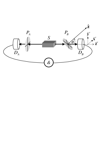
Figure 1: Scheme of the two-photon analyzer described in the text. $S$ is a source of Bell-Schmidt states, $P_{A}$ and $P_{B}$ are linear polarizers, and $D_{A}$ and $D_{B}$ are photo-detectors. The symbol & denotes the coincidence recorder.

In order to keep our treatment as general as possible, instead of considering a particular process-dependent scattered state, we focus our attention on the entanglement properties of the complete set provided by the Bell-Schmidt states Aravind (1995)

$$\begin{array}[]{ccc}|\Phi_{1}\rangle&=&\frac{1}{\sqrt{2}}(|x_{A},x_{B}\rangle+|y_{A},y_{B}\rangle),\\ \\ |\Phi_{2}\rangle&=&\frac{1}{\sqrt{2}}(|x_{A},x_{B}\rangle-|y_{A},y_{B}\rangle),\\ \\ |\Phi_{3}\rangle&=&\frac{1}{\sqrt{2}}(|x_{A},y_{B}\rangle+|y_{A},x_{B}\rangle),\\ \\ |\Phi_{4}\rangle&=&\frac{1}{\sqrt{2}}(|x_{A},y_{B}\rangle-|y_{A},x_{B}\rangle).\\ \end{array}$$ (94)

Then we associate to each Bell-Schmidt state a well defined photon momentum pair $(\mathbf{k}_{A},\mathbf{k}_{B})$ and we show that for each pure state $|\Phi_{i}\rangle$, the optimal choices of $\hat{\mathbf{a}},\hat{\mathbf{a}}^{\prime},\hat{\mathbf{b}}$ and $\hat{\mathbf{b}}^{\prime}$ depend on $(\mathbf{k}_{A},\mathbf{k}_{B})$ and therefore it is impossible to find a choice which is simultaneously optimal for all the states in the ensemble given in Eq. (93).

In order to demonstrate this, let us consider the detection coincidence scheme shown in Fig. 1. An idealized source $S$ emits photon pairs in the Bell-Schmidt states $|\Phi_{i}\rangle$. Two linear polarizers $P_{A}$ and $P_{B}$ are inserted in the paths of the two photons and two detectors $D_{A}$ and $D_{B}$ are put behind them. While $P_{A}$ is put perpendicular to the momentum $\mathbf{k}_{A}$ of the photon $A$, the axis $\hat{\mathbf{z}}$ of $P_{B}$ is such that $\hat{\mathbf{z}}\cdot\mathbf{k}_{B}/|\mathbf{k}_{B}|=\cos\theta$.

Aravind Aravind (1995) has shown that the choices $a_{z}=1$, $a^{\prime}_{x}=1$, $b_{y}=0=b_{y}^{\prime}$ are optimal for all the $|\Phi_{i}\rangle$, therefore we make the same assumptions. The remaining components of the two vectors $\hat{\mathbf{b}}$ and $\hat{\mathbf{b}}^{\prime}$ can be related to the physical orientations of the polarizer by writing,

$$\begin{array}[]{lcl}\hat{\mathbf{r}}&=&\mathrm{Tr}(T\bm{\sigma})\\ \\ &=&\bigl{\{}\mathrm{Tr}(T\sigma_{1}),\;\;0,\;\;\mathrm{Tr}(T\sigma_{3})\bigr{\}},\end{array}$$ (95)

where $\hat{\mathbf{r}}=\hat{\mathbf{b}},\hat{\mathbf{b}}^{\prime}$. $T$ is the polarizer Jones matrix as given in Eq. (49) and $\mathrm{Tr}(T\sigma_{2})=0$ because of the symmetry of $T$. Then we parameterize $\hat{\mathbf{b}}$ and $\hat{\mathbf{b}}^{\prime}$ by introducing the two angles $\beta$ and $\delta$ respectively, in the Eq. (95) obtaining

$$\begin{array}[]{lcl}\hat{\mathbf{b}}&=&\displaystyle{\left\{\frac{2\cos\theta\sin{\beta}\cos{\beta}}{1-\cos^{2}{\beta}\sin^{2}\theta},0,\frac{\cos^{2}\theta\cos^{2}{\beta}-\sin^{2}{\beta}}{1-\cos^{2}{\beta}\sin^{2}\theta}\right\}},\\ \\ \hat{\mathbf{b}}^{\prime}&=&\displaystyle{\left\{\frac{2\cos\theta\sin{\delta}\cos{\delta}}{1-\cos^{2}{\delta}\sin^{2}\theta},0,\frac{\cos^{2}\theta\cos^{2}{\delta}-\sin^{2}{\delta}}{1-\cos^{2}{\delta}\sin^{2}\theta}\right\}},\\ \end{array}$$ (96)

where ${\beta}$ stands for $\beta-\phi$ and ${\delta}$ for $\delta-\phi$. Now for each of the Bell-Schmidt states Eq. (94) we choose the values for ${\beta}$ and ${\delta}$ in order to maximize the violation of the Bell-CHSH inequality for $\theta=0$, and calculate

$$B_{i}(\theta)\equiv\mathrm{Tr}\bigl{(}\hat{\rho}_{i}\hat{\mathcal{B}}_{\mathrm{CHSH}}\bigr{)},\qquad(i=1,\ldots,4),$$ (97)

where we have defined $\hat{\rho}_{i}=|\Phi_{i}\rangle\langle\Phi_{i}|$. After a straightforward calculations one finds that $B_{1}(\theta)=B_{2}(\theta)$ and $B_{3}(\theta)=B_{4}(\theta)$, where

$$\begin{array}[]{lcl}B_{2}(\theta)&=&\displaystyle{-4\cos^{2}\left(\frac{\theta}{2}\right)\frac{1-(3+2\sqrt{2})\cos\theta}{1+(3+2\sqrt{2})\cos^{2}\theta}},\\ \\ B_{4}(\theta)&=&\displaystyle{4\cos^{2}\left(\frac{\theta}{2}\right)\frac{1-(3-2\sqrt{2})\cos\theta}{1+(3-2\sqrt{2})\cos^{2}\theta}}.\end{array}$$ (98)

These functions are plotted in Fig. 2.

Figure 2: Average Bell-CHSH operator $\langle\hat{\mathcal{B}}_{\mathrm{CHSH}}\rangle$ as a function of the polarizer “tilting” angle $\theta=\arccos(\hat{\mathbf{z}}\cdot\hat{\mathbf{k}}_{B})$, for the Bell-Schmidt states $|\Phi_{4}\rangle$ and $|\Phi_{2}\rangle$. The unit vectors $\hat{\mathbf{b}}$ and $\hat{\mathbf{b}}^{\prime}$ have been chosen such that for both states $\langle\hat{\mathcal{B}}_{\mathrm{CHSH}}\rangle=2\sqrt{2}$ for $\theta=0$. When $\theta$ increases, the violation of the Bell-CHSH inequality decreases. The same curves have been obtained for $|\Phi_{1}\rangle$ (alike $|\Phi_{2}\rangle$) and $|\Phi_{3}\rangle$, (alike $|\Phi_{4}\rangle$).

It is clear that the optimal choice $(\beta^{\mathrm{opt}}_{0},\delta^{\mathrm{opt}}_{0})$ at $\theta=0$, is no longer valid when $\theta$ increases and the degree of entanglement of skew photons appears to be reduced. However, one must realize that this loss of entanglement is an artefact due to our mismatched polarization detector. This means that it is still possible to find optimal values for $(\beta,\delta)$, but they will differ from the initial ones ($\theta=0$ case). In order to show this explicitly, we have investigated the dynamics of points $(\beta^{\mathrm{opt}},\delta^{\mathrm{opt}})$ in the plane $(\beta,\delta)$, for varying $\theta$. The results are shown in Fig. 3 in the case of $|\Phi_{4}\rangle$: for the other states the results are qualitatively similar.

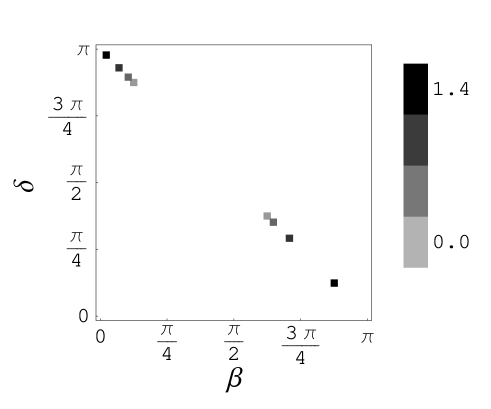
Figure 3: The square boxes represent points in the plane $(\beta,\delta)$ such that $\langle\hat{\mathcal{B}}_{\mathrm{CHSH}}\rangle=\pm 2\sqrt{2}$ ($+\Leftrightarrow$ lower series, $-\Leftrightarrow$ upper series) when the average is calculated with respect to $|\Phi_{4}\rangle$ for several values of $\theta$. When $\theta$ increases passing from zero (light grey) to about $\pi/2$ (dark grey), the “maximal violation points” move monotonically from light to dark along the line $\delta=\pi-\beta$.

When $\theta$ increases passing from zero to $\pi/2$ , the points $(\beta^{\mathrm{opt}},\delta^{\mathrm{opt}})$ move monotonically away from the central point $(\pi/2,\pi/2)$ along the line $\delta=\pi-\beta$ with different rates.

Figure 4: (a-b) Dependence of the optimal value of $\beta$ (such that $\langle\hat{\mathcal{B}}_{\mathrm{CHSH}}\rangle=2\sqrt{2}$), by the tilting angle $\theta$. For $\theta\gtrsim\pi/4$ different values of $\theta$ may require quite different values of $\beta$.

Once $\delta$ is fixed to the optimal value $\delta^{\mathrm{opt}}=\pi-\beta$, one can follow the motion of $\beta^{\mathrm{opt}}$ as a function of $\theta$. The dynamics is very simple and it is shown in Fig. 4. We list below the four functions $\beta^{\mathrm{opt}}_{i}(\theta)$, $(i=1,\dots,4)$ for reference:

$$\begin{array}[]{lcl}\beta^{\mathrm{opt}}_{1}(\theta)&=&-\arctan\left[(1-\sqrt{2}\cos\theta)\right],\\ \\ \beta^{\mathrm{opt}}_{2}(\theta)&=&\pi+\arctan\left[(1-\sqrt{2}\cos\theta)\right],\\ \\ \beta^{\mathrm{opt}}_{3}(\theta)&=&\arctan\left[(1+\sqrt{2}\cos\theta)\right],\\ \\ \beta^{\mathrm{opt}}_{4}(\theta)&=&\pi-\arctan\left[(1+\sqrt{2}\cos\theta)\right].\\ \end{array}$$ (99)

Despite their simplicity, Fig. 4 and Eqs. (99) tell us something important. We remind that the idealized experimental scheme we have considered in Fig. 1 was introduced to study the behavior of an entangled photon-pair in a statistical mixture in which each photon-pair has a well defined momentum. While in the above analysis we have considered $\theta$ as a free parameter representing the polarizer axis, in a real scattering experiment $\theta$ is the angle at which one of the photons, belonging to the entangled pair, impinges on the polarization detector. Then, each time a pair is scattered the two photons $A$ and $B$ will hit the detectors with arbitrary angles $\theta_{A}$ and $\theta_{B}$ respectively and the optimal polarizer orientation $\beta^{\mathrm{opt}}$ will be different for each couple of angles. Therefore it is clear that we cannot simultaneously optimize $\beta$ for all angles and the measured average degree of entanglement will be reduced independently from the scattering process considered. This completes our proof. Then we conclude that a conventional experimental setup for the measurement of the Bell-CHSH inequality, may fail to give the correct value for $\langle\hat{\mathcal{B}}_{\mathrm{CHSH}}\rangle$ when the measured state is a multi-mode scattered state.

V Summary and Outlook

The present paper aims to establish a theoretical background for a future study of scattering processes by both chaotic optical devices Aiello et al. (2003) and random media. The main concern of this paper has been to demonstrate that in a scattering process the measured degree of polarization-entanglement of a photon pair is unavoidably decreased because of the multi-mode detection. At the core of this loss of entanglement process resides the correlation between the momentum degrees of freedom and the polarization ones for the states of the electromagnetic field. In order to clarify the meaning of this correlation (or entanglement Peres (1998)), we have developed early on the paper a proper notation for the representation of the one-photon states of the electromagnetic field; this notation plays an important role throughout the paper. This introductory part also serves as a basis to show which dangers may be hidden behind the use of a misleading notation. In particular we show that the use of a reduced density matrix obtained by blindly tracing out the momentum degrees of freedom, can lead to a wrong result when applied to the calculation of a polarization-dependent observable.

The central part of this paper comprises two separate topics. The first topic consists in a careful analysis of the one-photon scattering processes. It is shown that a unique $2\times 2$ reduced density matrix is an useless concept for the analysis of a multi-mode scattering process, and that more information than this is required. The second topic is how to build, within the QED context, the one-photon states selected by an arbitrarily oriented linear polarizer. The knowledge of these states allows us to introduce the concept of the effective reduced density matrix which must be understood as the measured density matrix.

The last part of this paper is devoted to a brief introduction to the subject of the two-photon scattering processes and to the investigation of the Bell-CHSH inequality when, in a standard measurement setup, a polarization analyzer is arbitrarily tilted. The violation of the Bell-CHSH inequality is explicitly calculated for the complete Bell-Schmidt set of polarization-entangled states. We show that, when in a two-photon scattering experiment, the observer is ignorant about the momentum distribution of the scattered photons, he cannot find an optimal orientation for the polarizers in order to maximize the measured violation of the Bell-CHSH inequality. However this does not mean that a scattering process necessarily spoils the degree of entanglement of a given state, but instead just makes it not measurable with a standard measurement setup. This naturally raises a question about the physical meaning of a computable degree of entanglement which does not coincide with the measurable one. This topic is currently under investigation in our group Aie .