Storing and processing optical information with ultra-slow light in Bose-Einstein condensates

Abstract

We theoretically explore coherent information transfer between ultra-slow light pulses and Bose-Einstein condensates (BECs) and find that storing light pulses in BECs allows the coherent condensate dynamics to process optical information. We consider BECs of alkali atoms with a $\Lambda$ energy level configuration. In this configuration, one laser (the coupling field) can cause a pulse of a second pulsed laser (the probe field) to propagate with little attenuation (electromagnetically induced transparency) at a very slow group velocity ($\sim 10$ m/s), and be spatially compressed to lengths smaller than the BEC. These pulses can be fully stopped and later revived by switching the coupling field off and on. Here we develop a formalism, applicable in both the weak and strong probe regimes, to analyze such experiments and establish several new results: (1) We show that the switching can be performed on time scales much faster than the adiabatic time scale for EIT, even in the strong probe regime. We also study the behavior of the system changes when this time scale is faster than the excited state lifetime. (2) Stopped light pulses write their phase and amplitude information onto spatially dependent atomic wavefunctions, resulting in coherent two-component BEC dynamics during long storage times. We investigate examples relevant to Rb-87 experimental parameters and see a variety of novel dynamics occur, including interference fringes, gentle breathing excitations, and two-component solitons, depending on the relative scattering lengths of the atomic states used and the probe to coupling intensity ratio. We find the dynamics when the levels $|F=1,M_{F}=-1\rangle$ and $|F=2,M_{F}=+1\rangle$ are used could be well suited to designing controlled processing of the information input on the probe. (3) Switching the coupling field on after the dynamics writes the evolved BEC wavefunctions density and phase features onto a revived probe pulse, which then propagates out. We establish equations linking the BEC wavefunction to the resulting output probe pulses in both the strong and weak probe regimes. We then identify sources of deviations from these equations due to absorption and distortion of the pulses. These deviations result in imperfect fidelity of the information transfer from the atoms to the light fields and we calculate this fidelity for Gaussian shaped features in the BEC wavefunctions. In the weak probe case, we find the fidelity is affected both by absorption of very small length scale features and absorption of features occupying regions near the condensate edge. We discuss how to optimize the fidelity using these considerations. In the strong probe case, we find that when the oscillator strengths for the two transitions are equal the fidelity is not strongly sensitive to the probe strength, while when they are unequal the fidelity is worse for stronger probes. Applications to distant communication between BECs, squeezed light generation and quantum information are anticipated.

I Introduction

In discussions of quantum information technology quantumInfo , it has been pointed out that the ability to coherently transfer information between “flying” and stationary qubits will be essential. Atomic samples are good candidates for quantum storage and processing due to their long coherence times and large, controllable interactions, while photons are the fastest and most robust way to transfer information. This implies that methods to transfer information between atoms and photons will be important to the development of this technology.

Recently the observation of ultra-slow light (USL) Nature1 ; OtherUSL , propagating at group velocities more than seven orders of magnitude below its vacuum speed ($V_{g}\sim 10^{-7}c$), and the subsequent stopping and storing of light pulses in atomic media Nature2 ; OtherStoppedLight has demonstrated a tool to possibly accomplish this quantumProcessing . The technique relies on the concept of electromagnetically induced transparency (EIT)EIT in three level $\Lambda$-configuration atoms (see Fig. 1(a)). A coupling light field $\Omega_{c}$ is used to control the propagation of a pulse of probe light $\Omega_{p}$. The probe propagates at a slow group velocity and, as it is doing so, coherently imprints it’s amplitude and phase on the coherence between two stable internal states of the atoms, labelled $|1\rangle$ and $|2\rangle$ (which are generally particular hyperfine and Zeeman sublevels). Switching the coupling field off stops the probe pulse and ramps it’s intensity to zero, freezing the probe’s coherent (that is, intensity and phase) information into the atomic media, where it can be stored for a controllable time. Switching the coupling field back on at a later time writes the information back onto a revived probe pulse, which then propagates out of the atom cloud and can be detected, for example, with a photo-multiplier tube (PMT) (see Fig. 1(b)). In the original experiment Nature2 , the revived output pulses were indistinguishable in width and amplitude from non-stored USL pulses, indicating the switching process preserved the information in the atomic medium with a high fidelity.

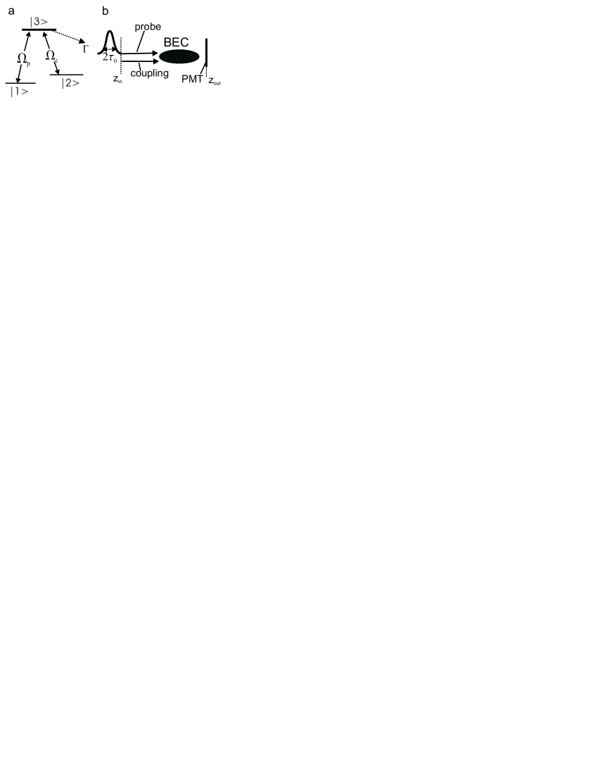
Figure 1: Schematic of ultra-slow light (USL) and stopped experiments. (a) The $\Lambda$ energy level structure which we consider has two stable states, $|1\rangle$ and $|2\rangle$, and an excited state $|3\rangle$ which decays at a rate $\Gamma$ (which is $(2\pi)~{}10$ MHz for Na and $(2\pi)~{}6$ MHz for Rb-87). Atoms which spontaneously decay from $|3\rangle$ are assumed to exit the levels under consideration. (b) We consider the two light fields to be co-propagating and input in the $+z$ direction (the long axis of the Bose-Einstein condensate (BEC)) at $z_{\mathrm{in}}$. The output intensity at $z_{\mathrm{out}}$ can be detected experimentally with a photo-multiplier tube (PMT). The probe field is pulsed with half-width $\tau_{0}$. The coupling beam is c.w. but can be switched off quickly to stop the probe pulse while it is in the BEC. Switching it back on later regenerates the probe light pulse.

In addition to the ability to store coherent information, compressing ultra-slow probe pulses to lengths shorter than the atomic cloud puts the atoms in spatially dependent superpositions of $|1\rangle$ and $|2\rangle$, offering novel possibilities to study two component BEC dynamics HauTalks . In SolitonVortex slow light pulses propagating in Bose-Einstein condensates (BECs) BEC of sodium were used to create density defects with length scales $\sim 2~{}\mu\mathrm{m}$, near the BEC healing length, leading to quantum shock waves and the nucleation of vortices.

Motivated by both observations of coherent optical information storage in atom clouds and the interesting dynamics which slow and stopped light pulses can induce in BECs, the present paper theoretically examines new possibilities offered by stopping light in BECs. We first present a novel treatment of the switching process and establish that the switch-off and switch-on of the coupling field can occur without dissipating the coherent information, provided the length scale of variations in the atomic wavefunctions are sufficiently large. We find that the switching of the coupling field can be done arbitrarily fast in the ultra-slow group velocity limit $V_{g}\ll c$. This is consistent with previous work Nature2 ; stoppedLight ; fastStopped ; stoppedTheory , but goes further as it applies to pulses in both the weak and strong probe regimes strongStopped . We also present the first explicit calculation of how the behavior of the system differs when one switches the coupling field faster than the natural lifetime of the excited state $\Gamma^{-1}$ (see Fig. 1(a)) and find the information is successfully transferred even in this regime. Furthermore we will see the analysis presented here, being phrased in terms of the spatial characteristics of the atomic wavefunctions, is well suited to addressing the issue of storage for times long compared to the time scale for atomic dynamics.

Investigation of this very issue of longer storage times constitute the central results of the paper. In this regime, there are important differences between optical information storage in BECs versus atom clouds above the condensation temperature (thermal clouds), which have been used in experiments to date. During the storage time, the light fields are off and the atomic wavefunctions evolve due to kinetic energy, the external trapping potential, and atom-atom interactions. (We label all these external dynamics to distinguish them from couplings between the internal levels provided by the light fields.) To successfully regenerate the probe pulse by then switching on the coupling field, there must be a non-zero value of the ensemble average (over all atoms) of the coherence between $|1\rangle$ and $|2\rangle$. When revivals were attempted after longer storage times in thermal clouds (several milliseconds in Nature2 ) the external dynamics had washed out the phase coherence between $|1\rangle$ and $|2\rangle$ (due to the atoms occupying a distribution of single particle energy levels) and no output pulses were observed. In zero temperature BECs the situation is completely different. There each atom evolves in an identical manner, described by a non-linear Schrodinger equation (Gross-Pitaevskii equation BEC ), preserving the ensemble average of the coherence during the external dynamics. That is, even as the amplitude and phase of the wavefunctions representing the BEC evolve, the relative phase of the two components continues to be well defined at all points in space. Thus, if we switch the coupling field back on, we expect that the evolved BEC wavefunctions will be written onto a revived probe field. In this way, the probe pulses can be processed by the BEC dynamics.

We show several examples, relevant to current Rb-87 BECs, of the interesting two component dynamics which can occur during the storage time. This atom possesses internal states with very small inelastic loss rates inelastic , and thus, long lifetimes multipleComponentJILA . We find that, depending upon the relative scattering lengths of the internal states involved and the relative intensity of the probe and coupling fields, one could observe the formation of interference fringes, gentle breathing motion, or the formation and motion of two-component (vector) solitons twoCompSolitons . In particular we find that using the levels $|F=1,M_{F}=-1\rangle$ and $|F=2,M_{F}=+1\rangle$ in Rb-87 could allow for long, robust storage of information and controllable processing. In each case, we observe the amplitude and phase due to the dynamical evolution is written onto revived probe pulses. These pulses then propagate out of the BEC as slow light pulses, at which point they can be detected, leaving behind a BEC purely in its original state $|1\rangle$.

For practical applications of this technique to storage and processing, one must understand in detail how, and with what fidelity, the information contained in the atomic coherence is transferred and output on the light fields. Thus, the last part of the paper is devoted to finding the exact relationship between the BEC wavefunctions before the switch-on and the observed output probe pulses. We find equations linking the two in the ideal limit (without absorption or distortion). Then, using our earlier treatment of the switching process, we identify several sources of imperfections and calculate the fidelity of the information transfer for Gaussian shaped wavefunctions of various amplitudes and lengths. In the weak probe limit, we find a simple relationship between the wavefunction in $|2\rangle$ and the output probe field. We find that optimizing the fidelity involves balancing considerations related to, on one hand, absorption of small length scale features in the BEC wavefunctions and, on the other hand, imperfect writing of wavefunctions which are too near the condensate edge. For stronger probes, we find a more complicated relationship, though we see one can still reconstruct the amplitude and phase of the wavefunction in $|2\rangle$ using only the output probe. In this regime, we find that the fidelity of the writing and output is nearly independent of the probe strength when the oscillator strengths for the two transitions involved ($|1\rangle\leftrightarrow|3\rangle$ and $|2\rangle\leftrightarrow|3\rangle$) are equal. However, unequal oscillator strengths lead to additional distortions and phase shifts, and therefore lower fidelity of information transfer, for stronger probes.

We first, in Section II, introduce a formalism combining Maxwell-Schrodinger and Gross-Pitaevskii equations BEC , which self-consistently describe both the atomic (internal and external) dynamics as well as light field propagation. We have written a code which implements this formalism numerically. Section III presents our novel analysis of the switching process, whereby the coupling field is rapidly turned off or on, and extends previous treatments of the fast switching regime, as described above. Section IV shows examples of the very rich variety of two-component dynamics which occur when one stops light pulses in BECs and waits for much times longer than the characteristic time scale for atomic dynamics. Section V contains our quantitative analysis of the fidelity with which the BEC wavefunctions are transferred onto the probe field. We conclude in Section VI and anticipate how the method studied here could eventually be applied to transfer of information between distant BECs, and the generation of light with squeezed statistics.

II Description of ultra-slow light in Bose-Einstein condensates

We first introduce our formalism to describe the system and review USL propagation within this formalism. Assume a Bose-condensed sample of alkali atoms, with each atom in the BEC containing three internal (electronic) states in a $\Lambda$-configuration (Fig. 1(a)). The states $|1\rangle$ and $|2\rangle$ are stable and the excited level $|3\rangle$, radiatively decays at $\Gamma$. In the alkalis which we consider, these internal levels correspond to particular hyperfine and Zeeman sublevels for the valence electron. When the atoms are prepared in a particular Zeeman sub-level and the proper light polarizations and frequencies are used Nature2 ; SolitonVortex , this three level analysis is a good description in practice. All atoms are initially condensed in $|1\rangle$ and the entire BEC is illuminated with a coupling field, resonant with $|2\rangle\leftrightarrow|3\rangle$ transition and propagating in the $+z$ direction (see Fig. 1(b)). A pulse of probe field, with temporal half-width $\tau_{0}$, resonant with the $|1\rangle\leftrightarrow|3\rangle$ transition, and also propagating in the $+z$ direction, is then injected into the medium. The presence of the coupling field completely alters the optical properties of the atoms as seen by the probe. What would otherwise be an opaque medium (typical optical densities of BECs are $\sim 400$) is rendered transparent via electromagnetically induced transparency (EIT) EIT , and the light pulse propagates at ultra-slow group velocities ($\sim 10$ m/s)Nature1 . As this occurs, all but a tiny fraction of the probe energy is temporarily put into the coupling field, leading to a compression of the probe pulse to a length smaller than the atomic medium itself Nature1 ; Nature2 ; HarrisHau .

To describe the system theoretically, we represent the probe and coupling electric fields with their Rabi-frequencies $\Omega_{p(c)}=-\mathbf{d}_{13(23)}\cdot\mathbf{E}_{p(c)}/\hbar$, where $\mathbf{E}_{p(c)}$ are slowly varying envelopes of the electric fields (both of which can be time and space-dependent) and $\mathbf{d}_{13(23)}$ are the electric dipole moments of the transitions. The BEC is described with a two-component spinor wavefunction $(\psi_{1},\psi_{2})^{T}$ representing the mean field of the atomic field operator for states $|1\rangle$ and $|2\rangle$. We ignore quantum fluctuations of these quantities, which is valid when the temperature is substantially below the BEC transition temperature FiniteTemp . The excited level $|3\rangle$ can be adiabatically eliminated adiabatic when the variations of the light fields’ envelopes are slow compared to the excited state lifetime $\Gamma^{-1}$ (which is 16 ns in sodium). The procedure is outlined in the Appendix. The functions $\psi_{1},\psi_{2}$ evolve via two coupled Gross-Pitaevskii (GP) equations BEC . For the present paper, we will only consider dynamics in the $z$ dimension, giving the BEC some cross-sectional area $A$ in the transverse dimensions over which all dynamical quantities are assumed to be homogeneous. This model is sufficient to demonstrate the essential effects here. We have considered effects due to the transverse dimensions, but a full exploration of these issue is beyond our present scope. The GP equations are SolitonVortex ; thesis :

$$i\hbar\frac{\partial\psi_{1}}{\partial t} = \bigg{[}-\frac{\hbar^{2}}{2m}\frac{\partial^{2}}{\partial z^{2}}+V_{1}(z)+U_{11}|\psi_{1}|^{2}+U_{12}|\psi_{2}|^{2}\bigg{]}\psi_{1}$$

$$-i\hbar\left(\frac{|\Omega_{p}|^{2}}{2\Gamma}\psi_{1}+\frac{\Omega_{p}^{\ast}\Omega_{c}}{2\Gamma}\psi_{2}\right),$$

$$i\hbar\frac{\partial\psi_{2}}{\partial t} = \bigg{[}-\frac{\hbar^{2}}{2m}\frac{\partial^{2}}{\partial z^{2}}+V_{2}(z)+U_{22}|\psi_{2}|^{2}+U_{12}|\psi_{1}|^{2}\bigg{]}\psi_{2}$$ (1)

$$-i\hbar\left(\frac{|\Omega_{c}|^{2}}{2\Gamma}\psi_{2}+\frac{\Omega_{p}\Omega_{c}^{\ast}}{2\Gamma}\psi_{1}\right),$$

where $m$ is the mass of the atoms and we will consider a harmonic external trapping potential $V_{1}(z)=\frac{1}{2}m{\omega_{z}}^{2}z^{2}$. The potential $V_{2}$ can in general differ from $V_{1}$. For example, in a magnetic trap the states $|1\rangle$ and $|2\rangle$ can have different magnetic dipole moments. However, in the examples we consider the potentials are equal to a good approximation, and so $V_{2}(z)=V_{1}(z)$ is assumed in the calculations. Atom-atom interactions are characterized by the $U_{ij}=4\pi N_{c}\hbar^{2}a_{ij}/mA$, where $N_{c}$ is the total number of condensate atoms and $a_{ij}$ are the s-wave scattering lengths for binary collisions between atoms in internal states $|i\rangle$ and $|j\rangle$. The last pair of terms in each equation represent the coupling via the light fields and give rise to both coherent exchange between $|1\rangle,|2\rangle$ as well as absorption into $|3\rangle$. In our model, atoms which populate $|3\rangle$ and then spontaneously emit are assumed to be lost from the condensate (Fig. 1(a)), which is why the light coupling terms are non-Hermitian.

The light fields’ propagation can be described by Maxwell’s equations. Assuming slowly varying envelopes in time and space (compared to optical frequencies and wavelengths, respectively) and with the polarization densities written in terms of the BEC wavefunctions these equations are SolitonVortex ; thesis :

$$\left(\frac{\partial}{\partial z}+\frac{1}{c}\frac{\partial}{\partial t}\right)\Omega_{p} = -\frac{N_{c}f_{13}\sigma_{0}}{2A}(\Omega_{p}|\psi_{1}|^{2}+\Omega_{c}{\psi_{1}}^{\ast}\psi_{2}),$$

$$\left(\frac{\partial}{\partial z}+\frac{1}{c}\frac{\partial}{\partial t}\right)\Omega_{c} = -\frac{N_{c}f_{23}\sigma_{0}}{2A}(\Omega_{c}|\psi_{2}|^{2}+\Omega_{p}\psi_{1}{\psi_{2}}^{\ast}),$$ (2)

where $f_{13},f_{23}$ are the dimensionless oscillator strengths of the transitions and $\sigma_{0}$ is the resonant cross section ($1.65\times 10^{-9}\mathrm{cm}^{2}$ and $2.91\times 10^{-9}\mathrm{cm}^{2}$ for the $D_{1}$ lines of sodium and Rb-87, respectively). These equations ignore quantum fluctuations of the light fields, just as the GP equations (II) ignore quantum fluctuations of the atomic fields. Note that in the absence of any coherence $\psi_{1}^{*}\psi_{2}$ these equations predict absorption of each field with the usual two-level atom resonant absorption coefficient (the atom density times the single atom cross-section).

For much of our analysis, we will solve Eqs. (II)-(II) self consistently with a numerical code, described in SolitonVortex ; thesis ; numerics . In SolitonVortex , this was successfully applied to predict and analyze the experimental observation of the nucleation of solitons and vortices via the light roadblock. When the light fields are off, the two states do not exchange population amplitude and Eqs. (II) reduce to coupled Gross-Pitaevskii equations for a two-component condensate. By contrast, when they are on and the probe pulse length $\tau_{0}$ (and inverse Rabi frequencies $\Omega_{p}^{-1},\Omega_{c}^{-1}$) are much faster than the time scale for atomic dynamics (typically $\sim$ ms), the internal couplings induced by the light field couplings will dominate the external dynamics.

For our our initial conditions, we consider $N_{c}\sim 10^{6}$ atoms are initially in $|1\rangle$ in the condensed ground state. We determine the wavefunction of this state $\psi_{1}^{(\mathrm{G})}(z)$ numerically by propagating (II) in imaginary time imaginaryTime , though the Thomas-Fermi approximation TF provides a good analytic approximation to $\psi_{1}^{(\mathrm{G})}(z)$. In the cases presented in this paper, we choose the transverse area $A$ so that the central density and chemical potential $\mu=U_{11}|\psi_{1}^{(\mathrm{G})}(0)|^{2}$ are in accordance with their values in a trap with transverse frequencies $\omega_{x}=\omega_{y}=3.8\,\omega_{z}$, as in previous experiments SolitonVortex . In Fig. 2 we consider an example with $N_{c}=1.2\times 10^{6}$ sodium atoms (with $a_{11}=2.75$ nm scatteringLengthNa ), $\omega_{z}=(2\pi)21~{}\mathrm{Hz}$ and $A=\pi(8.3~{}\mu\mathrm{m})^{2}$. The ground state density profile $N_{c}|\psi_{1}^{(\mathrm{G})}(z)|^{2}$ is indicated with the dotted curve in Fig. 2(b). In this case the chemical potential $\mu=(2\pi)~{}1.2~{}$kHz.

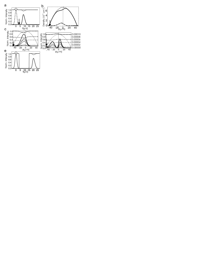
Figure 2: Coherent storage of a light pulse via fast switching. Results of numerical integration of Eqs. (II)-(II) showing both a slow and stopped light experiment. (a) The dashed curve shows the normalized input probe pulse intensity $|\Omega_{p}(z_{\mathrm{in}},t)|^{2}/\Omega_{p0}^{2}$ (a $\tau_{0}=1.5~{}\mu$s $1/e$ half-width, $\Omega_{p0}=(2\pi)~{}3.5~{}$MHz pulse), while the dotted curve shows $|\Omega_{c}(z_{\mathrm{in}},t)|^{2}/\Omega_{c0}^{2}$ for a constant input coupling field $\Omega_{c0}=(2\pi)~{}8.0~{}$MHz. The thick solid curve shows the delayed output probe pulse (at $z_{\mathrm{out}}$, see Fig. 1(b)). The time that the tail of the input has vanished and the rise of the output has not begun (marked by the arrow) corresponds to the time the pulse is completely compressed inside the BEC. In the output coupling intensity (thin solid curve) we see adiabatons. The values $\sigma_{0}=1.65\times 10^{-9}\,\mathrm{cm}^{2}$ and $f_{13}=1/2$ and $f_{23}=1/3$ have been used. (b) The atomic density in the two states, $N_{c}|\psi_{1}|^{2}/A$ (solid curve) and $N_{c}|\psi_{2}|^{2}/A$ (dashed curve), at $t=3.7~{}\mu$s (indicated by the arrow in (a)). The dotted curve shows the original density $N_{c}|\psi_{1}^{(\mathrm{G})}|^{2}/A$ before the probe is input. The arrow here and in (c)-(d) marks the position $z_{c}$ discussed later in the text. (c) Spatial profiles of the probe $|\Omega_{p}|^{2}/\Omega_{p0}^{2}$ (solid curves) and coupling $|\Omega_{c}|^{2}/\Omega_{c0}^{2}$ (dashed curves) field intensities at various times while the coupling field input is switched off. The switch-off is an error function profile with a width $\tau_{s}=0.1~{}\mu$s, centered at $t_{\mathrm{off}}=3.7\,\mu$s. Successively thinner curves refer to $t=3.52,3.65,3.68$, and $3.75\,\mu$s. The dotted curve indicates the original condensate density (arb. units). (d) Spatial profiles of the normalized dark $|\Omega_{D}|^{2}/\Omega_{c0}^{2}$ (dashed curves, scale on the left) and absorbed $|\Omega_{A}|^{2}/\Omega_{c0}^{2}$ (solid curves, scale on right) field intensities, at the same times as in (c). (e) The input and output probe and coupling intensities, with the same conventions as (a), in a stopped light simulation. In this case, the coupling field is switched off at $t_{\mathrm{off}}=3.7~{}\mu\mathrm{s}$ and then back on at $t_{\mathrm{on}}=15.3~{}\mu\mathrm{s}$.

With our initial ground state $\psi_{1}^{(\mathrm{G})}(z)$ determined, consider that we initially ($t=-\infty$) input a constant coupling field with a Rabi frequency $\Omega_{c0}$ and then inject a Gaussian shaped probe pulse at $z_{\mathrm{in}}$ (see Fig. 1(b)) with a temporal half-width $\tau_{0}$ and a peak Rabi frequency $\Omega_{p0}$. We define our times such that $t=0$ corresponds to the time the peak of the pulse is input. The dotted and dashed curves in Fig. 2(a) show, respectively, a constant coupling input $\Omega_{c0}=(2\pi)~{}8\,$MHz and a weaker input probe pulse with peak amplitude $\Omega_{p0}=(2\pi)3.5\,$MHz and width $\tau_{0}=1.5\,\mu$s.

Solving Eqs. (II)-(II) reveals that, when the conditions necessary for EIT hold, the pulse will compress upon entering the BEC and propagate with a slow group velocity. As it does this, it transfers the atoms into superpositions of $|1\rangle$ and $|2\rangle$ such that thesis :

$$\psi_{2}(z,t)\approx-\frac{\Omega_{p}(z,t)}{\Omega_{c}(z,t)}\psi_{1}(z,t),$$ (3)

which is a generalization to BECs of the single atom dark state darkState . Thus, the probe field $\Omega_{p}$ imprints its (time and space dependent) phase and intensity pattern in the BEC wavefunctions as it propagates. When (3) is exactly satisfied, it is easily seen that the two light field coupling terms in each of Eqs. (II) cancel, meaning that $|1\rangle$ and $|2\rangle$ are completely decoupled from the excited state $|3\rangle$. However, time dependence of $\Omega_{p}$ causes small deviations from (3) to occur, giving rise to some light-atom interaction which is, in fact, the origin of the slow light propagation. If one assumes the weak probe limit ($\Omega_{p0}\ll\Omega_{c0}$) and disregards terms of order $(\Omega_{p0}/\Omega_{c0})^{2}$ the group velocity of the probe pulse is HarrisHau ; thesis :

$$V_{g}(z)=\frac{\Omega_{c0}^{2}}{\Gamma}\frac{A}{N_{c}f_{13}\sigma_{0}|\psi_{1}^{(\mathrm{G})}(z)|^{2}}$$ (4)

and so is proportional the coupling intensity and inversely proportional to the atomic density $N_{c}|\psi_{1}^{\mathrm{(G)}}(z)|^{2}/A$. The half-width length of the pulse in the medium is $L_{p}=\tau_{0}V_{g}$, which is a reduction from it’s free space value by a factor $V_{g}/c$, while its peak amplitude does not change. Thus only a tiny fraction of the input probe pulse energy is in the probe field while it is propagating in the BEC. Most of the remaining energy coherently flows into the coupling field and exits the BEC, as can be seen in the small hump in the output coupling intensity (thin solid curve in Fig. 2(a)) during the probe input. This has been dubbed an adiabaton adiabatons . The magnitude of the adiabaton is determined by the intensity of the probe pulse.

In the weak probe limit $\psi_{1}(z,t)$ never significantly deviates from the ground-state wavefunction $\psi_{1}(z,t)\approx\psi_{1}^{(\mathrm{G})}(z)$ and the coupling field is nearly unaffected by the propagation $\Omega_{c}(z,t)\approx\Omega_{c0}$ (both of these results hold to $\mathcal{O}(\Omega_{p0}^{2}/\Omega_{c0}^{2})$). In this case (3) shows $\psi_{2}$ follows the probe field $\Omega_{p}$ as the pulse propagates. The arrow in Fig. 2(a) indicates a time where the probe has been completely input and has not yet begun to output. During this time, the probe is fully compressed in the BEC and Fig. 2(b) shows the atomic densities in $|1\rangle$ and $|2\rangle$ at this time. The spatial region with a non-zero density in $|2\rangle$ corresponds to the region occupied by the probe pulse (in accordance with (3)). Equation (3) applies to the phases as well as the amplitudes, however the phases in this example are homogenous and not plotted.

Once the pulse has propagated through the BEC, it begins to exit the $+z$ side. The energy coherently flows back from the coupling to probe field, and we see the output probe pulse (thick solid curve). Correspondingly, we see a dip in the coupling output at this time. In the experiments the delay between the input and output probe pulses seen in Fig. 2(a) is measured with a PMT (Fig. 1(b)). This delay and the length of the atomic cloud is used in to calculate the group velocity. The group velocity at the center of the BEC in the case plotted is $V_{g}(0)=6\,$m/s.

Note that the output pulse plotted in Fig. 2(a) at $z_{\mathrm{out}}$ is slightly attenuated. This reduction in transmission is due to the EIT bandwidth. The degree to which the adiabatic requirement $\tau_{0}\gg\Gamma/\Omega_{c0}^{2}$ is not satisfied, will determine the deviation the wavefunctions from the dark state (3), which leads to absorption into $|3\rangle$ and subsequent spontaneous emission. Quantitatively, this reduces the probe transmission (the time integrated output energy relative to the input energy) to thesis :

$$T=\frac{\int_{-\infty}^{\infty}dt\,|\Omega_{p}(z_{\mathrm{out}},t)|^{2}}{\int_{-\infty}^{\infty}dt\,|\Omega_{p}(z_{\mathrm{in}},t)|^{2}}=\frac{1}{\sqrt{1+4D(z_{\mathrm{out}})\left(\frac{\Gamma}{\tau_{0}\Omega_{c0}^{2}}\right)^{2}}},$$ (5)

where $D(z)=(N_{c}f_{13}\sigma_{0}/A)\int_{z_{\mathrm{in}}}^{z}dz^{\prime}|\psi_{1}^{\mathrm{(G)}}(z^{\prime})|^{2}$ is the optical density. In the Fig. 2 example, $D(z_{\mathrm{out}})=390$. The peak intensity of the pulse is reduced by a factor $T^{2}$ while the temporal width is increased by $T^{-1}$ (this spreading can be seen in Fig. 2(a)). The appearance of the large optical density $D(z_{\mathrm{out}})$ in (5) represents the cumulative effect of the pulse seeing a large number of atoms as it passes through the BEC. To prevent severe attenuation and spreading, we see we must use $\tau_{0}>\tau_{0}^{(\mathrm{min})}\equiv 2\sqrt{D(z_{\mathrm{out}})}\,\Gamma/\Omega_{c0}^{2}$, which is $1.0~{}\mu$s in our example.

III Fast switching and storage of coherent optical information

We now turn our attention to the question of stopping, storing and reviving probe pulses. We will show here that once the probe is contained in the BEC, the coupling field can be switched off and on faster than the EIT adiabatic time scale without causing absorptions or dissipation of the information Nature2 ; thesis . While we find no requirement on the time scale for the switching, we will obtain criteria on the length scales of $\psi_{1},\psi_{2}$ which must be maintained to avoid absorption events. While previous work Nature2 ; fastStopped ; stoppedTheory had addressed the fast switching case in the weak-probe limit, here we obtain results that are valid even when $\Omega_{p0}\sim\Omega_{c0}$ strongStopped . As we will see, for shorter storage times where the external atomic dynamics play no role, these length scale requirements can be related to the adiabatic requirements on the input probe pulse width $\tau_{0}$. The advantage of the current analysis is that it is easily applied to analyzing probe revivals after the atomic dynamics have completely altered the wavefunctions $\psi_{1},\psi_{2}$. In such a case it is these altered wavefunctions, rather than the input pulse width $\tau_{0}$, which is relevant.

III.1 Analyzing fast switching in the dark/absorbed basis

Consider that we switch the coupling field input off at some time $t_{\mathrm{off}}$ with a fast time scale $\tau_{s}\ll\tau_{0}$. Fig. 2(c) plots the probe and coupling intensities as a function of $z$ at various times during a switch-off with $\tau_{s}=0.1~{}\mu\mathrm{s}$. We see the probe intensity smoothly ramps down with the coupling field such that their ratio remains everywhere constant in time. Remarkably, for reasons we discuss below, the wavefunctions $\psi_{1},\psi_{2}$ are completely unaffected by this switching process. Motivated by this, we will, in the following, assume that $\psi_{1},\psi_{2}$ do not vary in time during this fast switching period, and later check this assumption.

To understand this behavior, it is useful to go into a dark/absorbed basis for the light fields, similar to that used in normalModes , by defining thesis :

$$\left(\begin{array}[]{c}\Omega_{D}\\ \Omega_{A}\end{array}\right) = \frac{1}{\psi_{0}}\left(\begin{array}[]{cc}-\psi_{2}^{*}&\psi_{1}^{*}\\ \psi_{1}&\psi_{2}\end{array}\right)\left(\begin{array}[]{c}\Omega_{p}\\ \Omega_{c}\end{array}\right),$$ (12)

where $\psi_{0}=\sqrt{|\psi_{1}|^{2}+|\psi_{2}|^{2}}$. From (12) one sees that when the condensate is in the dark state (3), $\Omega_{A}=0$. Using the notation $\psi_{i}=|\psi_{i}|e^{i\phi_{i}}$ and transforming the propagation equations (II) according to (12), one gets:

$$\bigg{(}\frac{\partial}{\partial z}+i\,\alpha_{l}\bigg{)}\Omega_{D} = \left(-\alpha_{NA}^{*}+\alpha_{12}^{*}\right)\Omega_{A}$$ (13)

$$\left(\frac{\partial}{\partial z}+\alpha_{A}-i\,\alpha_{l}\right)\Omega_{A} = \alpha_{NA}\Omega_{D},$$ (14)

where

$$\alpha_{A} \equiv \frac{N_{c}\sigma_{0}}{2A}\left(f_{13}|\psi_{1}|^{2}+f_{23}|\psi_{2}|^{2}\right),$$

$$\alpha_{12} \equiv \frac{N_{c}\sigma_{0}}{2A}(f_{13}-f_{23})\psi_{1}\psi_{2},$$

$$\alpha_{NA} \equiv \frac{1}{\psi_{0}^{2}}\bigg{[}\bigg{(}|\psi_{1}|\frac{d|\psi_{2}|}{dz}-|\psi_{2}|\frac{d|\psi_{1}|}{dz}\bigg{)}$$

$$\hskip 28.45274pt+i\bigg{(}\frac{d\phi_{2}}{dz}-\frac{d\phi_{1}}{dz}\bigg{)}|\psi_{1}||\psi_{2}|\bigg{]},$$

$$\alpha_{l} \equiv \frac{1}{\psi_{0}^{2}}\bigg{(}|\psi_{1}|^{2}\frac{d\phi_{1}}{dz}+|\psi_{2}|^{2}\frac{d\phi_{2}}{dz}\bigg{)},$$ (15)

and we have ignored the vacuum propagation terms $\sim 1/c$ in Eq. (II). They are unimportant so long as the fastest time scale in the problem is slow compared to time it takes a photon travelling at $c$ to cross the condensate (about $100~{}\mu\mathrm{m}/c\sim 1\,$ps). Note that $\alpha_{A}$ represents the usual absorption coefficient weighted according to the atomic density in each of $|1\rangle$ and $|2\rangle$. The terms $\alpha_{NA},\alpha_{l}$ arise from spatial variations in the wavefunctions, which make the transformation (12) space-dependent. The term $\alpha_{12}$ represents an additional effect present when the light-atom coupling coefficient differs on the two transitions ($f_{13}\not=f_{23})$ and is discussed in detail in Section V.3.

Consider for the moment a case with $f_{13}=f_{23}$ (implying $\alpha_{12}=0$) and assume a region in which $\psi_{1},\psi_{2}$ are homogenous (so $\alpha_{NA}=\alpha_{l}=0$). Equation (14) shows that the absorbed field $\Omega_{A}$ attenuates with a length scale $\alpha_{A}^{-1}$, the same as that for resonant light in a two-level atomic medium, and less than $1\,\mu$m at the cloud center for the parameters here. One would then get $\Omega_{A}\rightarrow 0$ after propagating several of these lengths. Conversely, (13) shows the dark light field $\Omega_{D}$ experiences no interaction with the BEC and propagates without attenuation or delay.

However, spatial dependence in $\psi_{1},\psi_{2}$ gives rise to $\alpha_{NA},\alpha_{l}\not=0$ in (13)-(14), introducing some coupling between $\Omega_{D}$ and $\Omega_{A}$, with the degree of coupling governed by the spatial derivatives $d\psi_{1}/dz,\,d\psi_{2}/dz$. A simple and relevant example to consider is the case of a weak ultra-slow probe pulse input and contained in a BEC, as discussed above (see Fig. 2(b)). The wavefunction $\psi_{2}$ has a homogenous phase and an amplitude which follows the pulse shape according to (3), meaning that $\alpha_{NA}$ scales as the inverse of the pulse’s spatial length $L_{p}^{-1}$.

It is important to note that this coupling is determined by spatial variations in the relative amplitude $\psi_{2}/\psi_{1}$ and does not get any contribution from variations in the total atomic density $\psi_{0}^{2}$. To see this we note that if we can write the wavefunctions as $\psi_{1}(z)=c_{1}\psi_{0}(z),\,\psi_{2}(z)=c_{2}\psi_{0}(z)$, where $c_{1},c_{2}$ are constants independent of $z$, then $\alpha_{NA}$ and $\alpha_{l}$ as defined in (III.1) vanish.

When variations in the relative amplitude are present, examination of (14) reveals that when the damping is much stronger than the coupling ($|\alpha_{NA}|,\alpha_{l}\ll\alpha_{A}$), one can ignore the spatial derivative term in analogy to an adiabatic elimination procedure. When we do this, (14) can be approximated by:

$$\Omega_{A}\approx\frac{\alpha_{NA}}{\alpha_{A}}\Omega_{D}$$ (16)

Strictly speaking, one can only apply this procedure in the region where $\Omega_{A}$ has propagated more than one absorption length (that is for $z>z_{c}$ where $z_{c}$ is defined by $\int_{z_{\mathrm{in}}}^{z_{c}}dz^{\prime}\alpha_{A}(z^{\prime})=1$). However, $z_{c}$ is in practice only a short distance into the BEC (marked with arrows in Figs. 2(b)-(d)). When the probe has already been input, as in Fig.2(b), $\psi_{2}$ and therefore $\Omega_{A}$ (see (12)) are already trivially zero for $z<z_{c}$ so (16) holds everywhere. We next plug Eq. (16) into Eq. (13), giving:

$$\frac{\partial\Omega_{D}}{\partial z}=\left[-\frac{|\alpha_{NA}|^{2}}{\alpha_{A}}+\frac{\alpha_{NA}\alpha_{12}^{*}}{\alpha_{A}}-i\,\alpha_{l}\right]\Omega_{D}.$$ (17)

These last two equations rely only on assumptions about the spatial derivatives of $\psi_{1},\psi_{2}$ and not on the time scale of the switch-off $\tau_{s}$ (though we have assumed $\tau_{s}\gg\Gamma^{-1}$ in adiabatically eliminating $|3\rangle$ from our original Eqs. (II)-(II)).

These results allow us to conclude two important things which hold whenever $|\alpha_{NA}|,\alpha_{l}\ll\alpha_{A}$ and the probe has been completely input. First, the coefficients governing the propagation of $\Omega_{D}$ in (17) are extremely small. The length scales $|\alpha_{NA}|^{-1},\alpha_{12}^{-1}$ are already generally comparable to the total BEC size and the length scales for changes in $\Omega_{D}$, given by (17), scale as these terms multiplied by the large ratio $\alpha_{A}/\alpha_{NA}$. (The $\alpha_{l}$ term in (17) can lead to additional phase shifts, which we discuss in Section V.3). Therefore the dark field $\Omega_{D}$ propagates with very little attenuation. As we have noted (and later justify and discuss in more detail) the wavefunctions (and therefore the propagation constant in brackets in (17)) are virtually unchanged during the switch-off. Under this condition, changes initiated in $\Omega_{D}$ at the entering edge $z_{\mathrm{in}}$ quickly propagate across the entire BEC. To apply this observation to the switch-off, we note when the pulse is contained so $\psi_{2}=0$ at the entering edge, (12) shows $\Omega_{D}=\Omega_{c}$ there. Switching off the coupling field at $z_{\mathrm{in}}$ then amounts to switching off $\Omega_{D}$ at $z_{\mathrm{in}}$ and (17) shows that this switch-off propagates through the entire BEC with little attenuation or delay. Second, from (16) we see that as $\Omega_{D}$ is reduced to zero $\Omega_{A}$ is reduced such that the ratio $\Omega_{A}/\Omega_{D}$ remains constant in time.

A numerical simulation corroborating this behavior is plotted in Fig. 2(d). The dark field intensity $|\Omega_{D}|^{2}$ is seen to switch-off everywhere as the coupling field input is reduced to zero over a $\tau_{s}=0.1\,\mu$s timescale, confirming that the changes in the input propagate across the BEC quickly and with little attenutation. The ratio $|\Omega_{A}|^{2}/|\Omega_{D}|^{2}$ is everywhere much smaller than unity and constant in time. The only exception to this is in a small region $z<z_{c}$ at the cloud entrance, where $\Omega_{A}$ has not yet been fully damped. The plot of $|\Omega_{A}|^{2}$ during the switch-off indeed demonstrates how (16) is a generally good approximation, but breaks down in this region. In the case plotted (and any case where the probe is fully contained) the wavefunction $\psi_{2}$ is so negligible in this region that $\Omega_{A}$ is rather small and unimportant (note the scale on the right hand side of the plot).

Translating this back into the $\Omega_{p},\Omega_{c}$ basis, we note from (12) that keeping $\Omega_{A}\approx 0$ means the probe must (at all $z$) constantly adjust to the coupling field via:

$$\Omega_{p}=-\left(\frac{\psi_{2}}{\psi_{1}}\right)\Omega_{c}$$ (18)

Thus we see that $\Omega_{p}$ smoothly ramps down with $\Omega_{c}$ even if $\Omega_{c}$ is ramped down quickly, as seen in Fig. 2(c).

Using our results for the light fields, we can now see why the wavefunctions $\psi_{1},\psi_{2}$ do not change during the switching. Physically, the probe is in fact adjusting to maintain the dark state (18), and in doing so induces some transitions between $|1\rangle$ and $|2\rangle$. However, only a fraction $V_{g}/c\sim 10^{-7}$ of the input energy is in the probe while it is contained in the medium, and so the probe is completely depleted before any significant change occurs in $\psi_{1},\psi_{2}$ Nature2 . In fact, the energy content of the probe field right before the switch-off is less than 1/100th of a free-space photon in the case here. Thus, $\Omega_{p}$ is completed depleted after only a fraction of one $|1\rangle\rightarrow|2\rangle$ transition. Note that (18) is equivalent to (3). However, writing it in this way emphasizes that, during the switching, the probe is being driven by a reservoir consisting of the coupling field and atoms and adjusts to establish the dark state. This is contrast to the situation during the probe input, when many photons from both fields are being input at a specific amplitude ratio, forcing the atomic fields to adjust to establish the appropriate dark state. Plugging in our results for the light fields (16)-(17) into our Eqs. (II) we can calculate the changes that occur in $\psi_{1}$ and $\psi_{2}$ during the switch-off. Doing this, we find relative changes in $\psi_{1},\psi_{2}$ are both smaller than $\tau_{s}/\tau_{0}$, which can be made arbitrarily small for fast switching $\tau_{s}\ll\tau_{0}$. The little change which does occur is due not to any process associated with the switching itself but is due to the small amount of propagation during the switch-off. It is therefore safe to assume (as we saw numerically) that $\psi_{1},\psi_{2}$ are constant in time during the switch-off. One can also show with this analysis that the ratio of coherent exchange events (from $|1\rangle$ to $|2\rangle$ or vice-versa) to absorptive events (transitions to $|3\rangle$ followed by spontaneous emission) is $|\Omega_{D}/\Omega_{A}|$ implying that the switch-off occurs primarily via coherent exchanges.

In the original stopped light experiment Nature2 , the coupling field was then switched back on to $\Omega_{c0}$, after some controllable storage time $\tau_{st}$, at a time $t_{\mathrm{on}}=t_{\mathrm{off}}+\tau_{st}$. In that experiment, revivals were observed for storage times $\tau_{st}$ too short for significant external atomic dynamics to occur, so the state of the atoms was virtually identical at $t_{\mathrm{on}}$ and $t_{\mathrm{off}}$. Then the analysis of the switch-on is identical to the switch-off as it is just the same coherent process in reverse. The probe is then restored to the same intensity and phase profile as before the switch-off. An example of such a case is plotted in Fig. 2(e). The output revived pulse then looks exactly like the normal USL pulse (compare the output in Figs. 2(a),(e)), as was the case in the experiment.

We have established the requirement $|\alpha_{NA}|\ll\alpha_{A}$ is necessary and sufficient for coherent switching to occur. Under what conditions is this satisfied? When the switch-off occurs while the probe is compressed, it is always satisfied because of bandwidth considerations mentioned above (see Eq. (5)). Specifically, the input pulse must satisfy $\tau_{0}>\tau_{0}^{(\mathrm{min})}$. However, this leads to a pulse width in the medium of $L_{p}>2\sqrt{D(z_{\mathrm{out}})}\,\alpha_{A}^{-1}$, implying that $|\alpha_{NA}|\ll\alpha_{A}$ is satisfied (as $D(z_{\mathrm{out}})\gg 1$). Therefore, any pulse which can successfully propagate to the cloud center, can be abruptly stopped and coherently depleted by a rapid switch-off of the coupling field. Of course, if the switch-on is then done before significant atomic dynamics, the same reasoning applies then. In this case, our requirements on the spatial derivatives are already encapsulated by the adiabatic requirements on the probe pulse. It is when the external atomic dynamics during the storage significantly change $\psi_{1},\psi_{2}$, that the analysis of the switch-on becomes more complicated. This is the central purpose of the Sections IV-V below.

As hinted above, when the pulse is not yet completely input, the switching can cause absorptions and dissipation of the information. In this case $\psi_{2}$ is significant in the region $z<z_{c}$ and so $\Omega_{A}$ is significant for several absorption lengths into the BEC. Physically, the coupling field sees atoms in a superposition of $|1\rangle$ and $|2\rangle$ immediately upon entering the condensate rather than only $|1\rangle$ atoms. Numerical simulations of this situation confirm this. During both the switch-on and switch-off, a significant number of atoms are lost from both condensate components, primarily concentrated in the $z<z_{c}$ region, and the revived probe pulse is significantly attenuated relative to the pulse before the storage.

Incidentally, this explains the apparent asymmetry between the probe and coupling in a stopped light experiment. Whenever both fields are being input, the temporal variations in both fields must be slow compared with the EIT adiabatic time scale, as the atomic fields must adjust their amplitudes to prevent absorptions. However, when one of the fields is no longer being input (like a contained probe pulse), the other field’s input can be quickly varied in time.

III.2 Switching faster than $\Gamma^{-1}$

When the switching is done quickly compared to the natural lifetime of $|3\rangle$ ($\tau_{s}<\Gamma^{-1}$), the assumptions needed for adiabatic elimination of $\psi_{3}$ are no longer valid. The analysis of the switching then becomes more complicated but, remarkably, we find the quality of the storage is not reduced in this regime.

To see this, we performed numerical simulations of switching in this regime by solving Eqs. (31)-(A) (which are the analogues of (II)-(II) without the adiabatic elimination of $\psi_{3}$) for the same parameters as Fig. 2 but varying $\tau_{s}$ from $80~{}\mathrm{ns}$ to $0.1~{}\mathrm{ns}$ numerics3Comp . An example with $\tau_{s}=2~{}\mathrm{ns}$ is shown in Fig. 3. We plot the probe and coupling amplitudes versus time at a point near the center of the BEC, and zoom in on the regions near the switch-on and -off. Note that that while the coupling field smoothly varies to it’s new value in each case, the probe field slightly overshoots the value given by (18) before returning to it. In all cases with $\tau_{s}<\Gamma^{-1}$ the probe amplitude $|\Omega_{p}|$ experienced damped oscillations before reaching its final value. The frequency of the oscillations was determined by $\tau_{s}^{-1}$ and the damping rate was $\Gamma$.

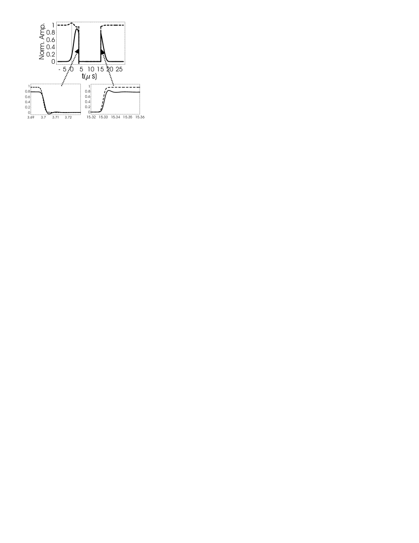
Figure 3: Switching faster than the natural linewidth. Solid and dashed lines show, respectively, the normalized probe and coupling amplitudes at a point in the center of the BEC $\Omega_{p}(z=-12~{}\mu\mathrm{m},t)/\Omega_{p0},\;\Omega_{c}(z=-12~{}\mu\mathrm{m},t)/\Omega_{c0}$ when the switching is faster than the natural linewidth $\tau_{s}=2~{}\mathrm{ns}\ll\Gamma^{-1}$ (but otherwise the same parameters as Fig. 2(e)). The two insets magnify the regions near the $t_{\mathrm{off}}$ and $t_{\mathrm{on}}$.

During these oscillations, the absorbing field $\Omega_{A}$ is in fact quite significant. However, the maximum value of $|\psi_{3}|$ and the total atomic loss due to spontaneous emissions events was completely independent of $\tau_{s}$ over the range we explored. To understand this, we note that even though $\Omega_{A}$ is larger, the frequency components of the quickly varying coupling field are spread over a range much wider than $\Gamma$. Thus a very small fraction of the energy in the field $\Omega_{c}$ is near resonant with the atomic transition and it passes through the BEC unattenuated. Analyzing the problem in Fourier space one can see that the increase in $\Omega_{A}$ for smaller $\tau_{s}$ is precisely offset by this frequency width effect, leading us to the conclusion that spontaneous emission loss is independent of $\tau_{s}$.

Unlike the case of switching slowly compared with $\Gamma^{-1}$, the adjustment of the probe is not a coherent process. Rather, spontaneous emission damps the system until the dark state (18) is reached. However, because we are in the regime $V_{g}\ll c$ the amount of energy in the probe is much less than one photon, and thus still has virtually no impact on $\psi_{1},\psi_{2}$. This will not necessarily hold when $V_{g}\sim c$ and in stoppedTheory it was predicted that there are, in fact, adiabatic requirements for $\tau_{s}$ in this regime. However, in all cases of interest here this inequality is well satisfied and there is no restriction on $\tau_{s}$.

IV BEC dynamics and processing optical information

We now turn to the question of the atomic dynamics during the storage time. These dynamics depend strongly on the relative scattering lengths of the states used, and the probe to coupling intensity ratio. We will see that the these dynamics are written onto revived probe pulses by switching the coupling field back on. The length scale requirement on variations in the relative amplitude $\psi_{2}/\psi_{1}$ derived above ($|\alpha_{NA}|\ll\alpha_{A}$) plays a central role in the fidelity with which these dynamics are written. We will demonstrate with several examples, relevant to current Rb-87 experimental parameters.

IV.1 Writing from wavefunctions onto light fields

In Nature2 the revived pulses were seen to be attenuated for longer storage times with a time constant of $\sim 1$ ms. The relative phase between the $|1\rangle$ and $|2\rangle$ (or coherence), averaged over all the atoms, washed out because the atoms, although at a cold temperature of $0.9~{}\mu\mathrm{K}$, were above the Bose-condensation temperature and so occupied a distribution of energy levels. By contrast, a zero temperature two-component BEC will maintain a well defined phase (the phase between $\psi_{1}$ and $\psi_{2}$) at all $z$, even as $\psi_{1},\psi_{2}$ evolve. They evolve according to the two-component coupled GP equations (II) with the light fields set to zero ($\Omega_{p}=\Omega_{c}=0$), and the initial conditions are determined by the superposition created by the input pulse at $t_{\mathrm{off}}$ (see Fig. 2(b)). After such an evolution, we can then switch the coupling field back on and the probe will be revived according to (18) but with the new wavefunctions $\psi_{1},\psi_{2}$, evaluated at $t_{\mathrm{on}}$.

Here we examine a wide variety of different two-component BEC dynamics which can occur after a pulse has been stopped. Because of the initial spatial structure of $\psi_{1},\psi_{2}$ created with the USL pulses, we see some novel effects in the ensuing dynamics.

Upon the switch-on, in many cases the probe will be revived via (18). We label the spatial profile of the revived probe by $\Omega_{p}^{(\mathrm{rev})}(z)\equiv\Omega_{p}(z,t_{\mathrm{on}}+\tau_{s})$. When we are in the weak probe limit ($|\Omega_{p}|\ll|\Omega_{c}|$ or, stated in terms of the wavefunctions, $|\psi_{2}|\ll|\psi_{1}|$), (18) becomes

$$\Omega_{p}^{(\mathrm{rev})}(z)=-\frac{\psi_{2}(z,t_{\mathrm{on}})}{\psi_{1}^{\mathrm{(G)}}(z)}\Omega_{c0}.$$ (19)

allowing us to make a correspondence between the revived probe and $\psi_{2}$ if $\Omega_{c0}$ and $\psi_{1}^{\mathrm{(G)}}(z)$ are known. The revived pulse will then propagate out of the BEC to the PMT at $z_{\mathrm{out}}$. In the absence of any attenuation or distortion during the propagation out, the spatial features of the revived probe get translated into temporal features. Thus if we observe the output $\Omega_{p}^{(\mathrm{out})}(t)\equiv\Omega_{p}(z_{\mathrm{out}},t)$ then we would deduce that revived pulse was

$$\Omega_{p}^{(\mathrm{rev})}(z)=\Omega_{p}^{(\mathrm{out})}\big{(}\tau(z_{\mathrm{out}})-\tau(z)+t_{\mathrm{on}}\big{)}$$ (20)

where $\tau(z_{\mathrm{out}})-\tau(z)\equiv(\Gamma/\Omega_{c0}^{2})(D(z_{\mathrm{out}})-D(z))$ is the time it takes the probe pulse to travel from some point $z$ to $z_{\mathrm{out}}$. Note that we are relying here on the fact that we can switch the coupling field onto its full value of $\Omega_{c0}$ with a time scale fast compared to the pulse delay times $\tau(z_{\mathrm{out}})-\tau(z)$. A slow ramp up would lead to a more complicated relationship between $\Omega_{p}^{(\mathrm{rev})}(z)$ and $\Omega_{p}^{(\mathrm{out})}(t)$.

Combining (19) and (20) shows how the phase and amplitude information that was contained in $\psi_{2}$ at the time of the switch-on is transferred to the output probe $\Omega_{p}^{(\mathrm{out})}(t)$. This transfer will be imperfect for three reasons. First, when sufficiently small spatial features are in $\psi_{2}$, then $\alpha_{NA}$ is comparable to $\alpha_{A}$, giving rise to a significant $\Omega_{A}$. The resulting absorptions will cause deviations of $\Omega_{p}^{(\mathrm{rev})}$ from our expectation (19). Second, we mentioned how spatial features are translated into temporal features on the output probe. During the output, fast time features on the output probe will be attenuated via the bandwidth effect discussed in (5), affecting the accuracy of the correspondence (20). Finally, stronger output probes, which will occur when $|\psi_{2}|\sim|\psi_{1}|$ at the time of the switch-on, make both the writing at the switch-on and the subsequent propagation out more complicated and less reliable. Our following examples will demonstrate these considerations.

IV.2 Formation and writing of interference fringes

Interesting dynamics occur in when the two internal states are trapped equally ($V_{2}=V_{1}$) and the scattering lengths $a_{12},a_{11}$ are slightly different. We consider a case with $N_{c}=1.0\times 10^{6}$ Rb-87 atoms and choose $|1\rangle=|5S_{1/2},F=2,M_{F}=+1\rangle$, $|2\rangle=|5S_{1/2},F=1,M_{F}=-1\rangle$, and $|3\rangle=|5P_{1/2},F=2,M_{F}=0\rangle$. The two lower states $|1\rangle$ and $|2\rangle$ are magnetically trapped with nearly identical magnetic moments, and we consider a trap with $\omega_{z}=(2\pi)~{}21~{}\mathrm{Hz}$ and assume a tranvserse area $A=\pi(5~{}\mu\mathrm{m})^{2}$. These two states have an anomalously small inelastic collisional loss rate inelastic and so have been successfully used to study interacting two-component condensates for hundreds of milliseconds multipleComponentJILA . The elastic scattering lengths are $a_{11}=5.36~{}\mathrm{nm},\,a_{12}=1.024\,a_{11},\,a_{22}=1.057\,a_{11}$ scatteringLengthRb .

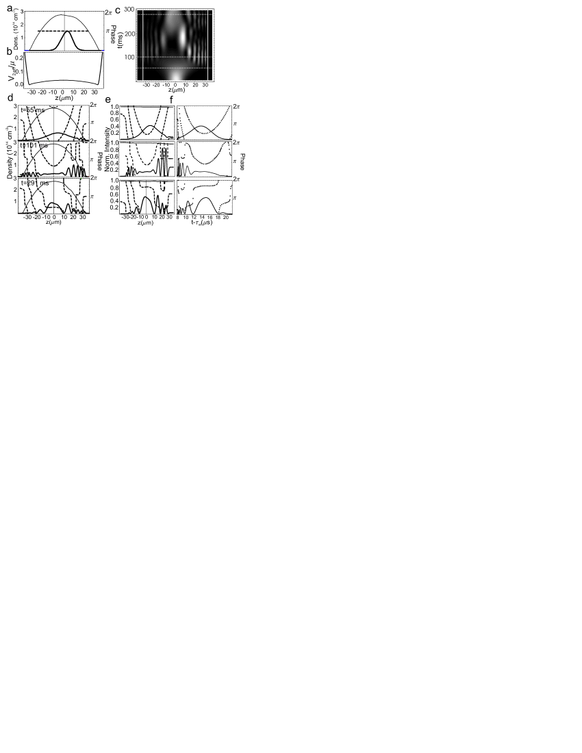
Figure 4: Formation of interference fringes in Rb-87 and writing fringes to probe light field. (a) The initial wavefunctions created by a $\tau=2.0~{}\mu\mathrm{s},\,\Omega_{p0}=(2\pi)~{}2~{}\mathrm{MHz}$ probe pulse. The coupling field is initially on at $\Omega_{c0}=(2\pi)~{}8~{}\mathrm{MHz}$ then switched off at $t_{\mathrm{off}}=7.5~{}\mu\mathrm{s}$. The cloud parameters and atomic levels are described in the text. The thick solid curve shows the density $N_{c}|\psi_{2}(z)|^{2}/A$ (multiplied by 10 for clarity) while the thick dashed curve shows the phase $\phi_{2}(z)$. The thin curve shows the density $N_{c}|\psi_{1}(z)|^{2}/A$. The phase $\phi_{1}$ is approximately homogenous and not shown. (b) The effective potential $V_{\mathrm{2-eff}}/\mu$ (21) seen by the condensate in $|2\rangle$. (c) The resulting evolution of the density $N_{c}|\psi_{2}(z,t)|^{2}/A$ (white represents higher density) as the wave packet is pushed down the both sides of potential hill and interferes with itself upon reaching the hard wall in $V_{\mathrm{2-eff}}$ at the condensate edge. The vertical grey lines show the condensate boundary, and the horizontal grey lines indicate the times plotted in (d). (d) Plots of the density and phase of the wavefunctions at the indicated times (with the same conventions as (a)) at $t=55~{}\mathrm{ms},101~{}\mathrm{ms}$ and $291~{}\mathrm{ms}$. (e) Spatial profiles of the probe and coupling field directly after a fast switch-on after a storage time $\tau_{st}=t_{\mathrm{on}}-t_{\mathrm{off}}$ corresponding to the times in (d). The thick (thin) solid curves show the intensities $|\Omega_{p}^{\mathrm{(rev)}}(z)/\Omega_{p0}|^{2}\,(|\Omega_{c}(z)/\Omega_{c0}|^{2})$ and the dashed curve shows the phase $\phi_{p}^{\mathrm{(rev)}}$ ($\phi_{c}$ is nearly homogenous and not plotted). (f) The time profile of the probe output intensity (solid curve) and phase (dots) at the output $z_{\mathrm{out}}$.

Figure 4(a) shows the initial wavefunctions $\psi_{1},\psi_{2}$ after the input and stopping of a probe pulse. We see a Gaussian shaped density profile in $|2\rangle$ reflecting the input probe’s Gaussian shape. The subsequent dynamics are governed by Eqs. (II) with $\Omega_{p}=\Omega_{c}=0$. In this case, a weak probe ($\Omega_{p0}^{2}=\Omega_{c0}^{2}/16$) was input. As a result, $\psi_{1}(z,t)\approx\psi_{1}^{(\mathrm{G})}(z)$ is nearly constant in time and the evolution of $\psi_{2}$ is governed by essentially linear dynamics, with a potential determined by the magnetic trap and interactions with $|1\rangle$ atoms:

$$V_{2-\mathrm{eff}}(z)=V_{2}(z)+U_{12}|\psi_{1}^{(\mathrm{G})}(z)|^{2}-\mu.$$ (21)

Figure 4(b) shows this potential in this case. The hill in the middle has a height $\mu[(a_{12}-a_{11})/a_{11}]$ and arises because atoms feel a stronger repulsion from the condensate in $|1\rangle$ when they are in $|2\rangle$. Figures 4(c-d) show the subsequent dynamics. One sees that the $|2\rangle$ condensate is pushed down both sides of the potential hill and spreads. However, once it reaches the border of the BEC, it sees sharp walls from the trap potential. Even for the fairly moderate scattering length difference here, there is sufficient momentum acquired in the descent down the hill to cause a reflection and formation of interference fringes near the walls. The wavelength of the fringes is determined by this momentum.

What happens if one switches the coupling field back on after these dynamics? Figures 4(e) shows the revived probe pulses $\Omega_{p}^{(\mathrm{rev})}(z)$ upon switch-ons at the times corresponding to Fig. 4(d). One sees a remarkable transfer of the sharp density and phase features of the $|2\rangle$ condensate onto the probe field, according to (19). Because we are in the weak probe regime, the coupling field intensity only very slightly deviates from it’s input value $\Omega_{c0}$. Figures 4(f) then shows the output probe $\Omega_{p}^{(\mathrm{out})}(t)$. The sharp interference fringes are able to propagate out, though there is some attenuation and washing out of the features. Note that the features at more positive $z$ propagate out first, leading to a mirror image-like relationship between the spatial Fig. 4(e) and temporal Fig. 4(f) patterns as predicted by (20).

In this particular example, we successfully output many small features from the $\psi_{2}$ to the output probe field. Here the fringes are $\sim 3~{}\mu\mathrm{m}$, which is still larger than the absorption length $\sim 0.5~{}\mu\mathrm{m}$, but not substantially so, leading to some small amount of dissipation during the switch-on and output. This gives us a sense of the “information capacity”. The number of absorption lengths, or optical density, which in this case is $D(z_{\mathrm{out}})\approx 300$, ultimately limits the number of features (for a given desired fidelity) which could be successfully written and output. Note also that in the $\tau_{st}=101~{}\mathrm{ms}$ case, some of the $\psi_{2}$ amplitude occupies the entering region $(z<z_{c})$ leading to additional imperfections in the writing process in this region.

IV.3 Breathing behavior and long storage

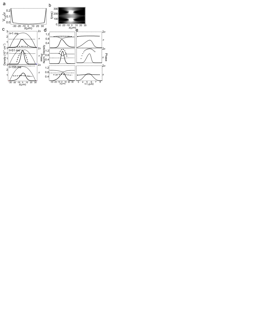
Figure 5: Breathing behavior and long storage In this case the states chosen for $|1\rangle$ and $|2\rangle$ are reversed, changing the sign of the curvature in the effective potential (21) in (a). All plots are the plotted with the same conventions as Fig. 4 except we additionally plot thin dotted curves in (c) showing the phase $\phi_{1}(z)$ and in (d) showing the phase $\phi_{c}(z)$.

The dynamics in the previous example are quite dramatic, but are not particularly conducive to preserving or controllably processing the information in the BEC. For this, it would be preferable to switch the roles of $|1\rangle$ and $|2\rangle$. Such a case is shown in Fig. 5. Because $a_{12}<a_{11}$ in this case, the potential hill is turned into a trough (see Fig. 5(a)). The effective potential in the region of the $|1\rangle$ condensate, in the Thomas-Fermi limit, becomes $V_{2-\mathrm{eff}}=V_{1}[(a_{11}-a_{12})/a_{11}]$ and so it harmonic, with a much smaller oscillator frequency than the magnetic trap. The evolution can be easily calculated by decomposing the wavefunction $\psi_{2}$ into a basis of the harmonic oscillator states of this potential. In the example here, there is significant occupation of the first several oscillator levels, and so one sees an overall relative phase shift in time (from the ground state energy of the zeroeth state), a slight dipole oscillation (from occupation of the first excited state) and breathing (from the second). After one oscillator period (310 ms in the case shown), $\psi_{2}$ replicates its original value at the switch-off.

In this case, the dynamics are quite gentle, and so the spatial scales of the phase and density features are always quite large compared with the absorption length $\alpha_{A}^{-1}$. The fidelity of the writing and output of the information on the probe field (shown in Figs. 5(d-e)) is correspondingly better than in the previous example. Additionally, because the $|2\rangle$ is trapped near the BEC center, this case avoids problems associated with $\psi_{2}$ occupying the region $z<z_{c}$.

Because of both the ease of analyzing the evolution and the high fidelity of outputting the information, we expect this case to be well-suited to controlled processing of optical information. For example, if the input pulse created a wavefunction $\psi_{2}$ corresponding to the ground state of the oscillator potential, the evolution would result only in a homogenous phase shift, proportional to the storage time, allowing long storage of the information or introduction of controllable phase shifts. By choosing the pulse lengths differently so several oscillator states are occupied, one could achieve linear processing or pulse reshaping.

Furthermore, note that in this example there is a small but discernable dip in the $|1\rangle$ density at 51 ms, indicating some nonlinearity in the evolution of $\psi_{2}$. One can tune this nonlinearity by varying the probe to coupling ratio, leading to nonlinear processing of the information.

IV.4 Strong probe case: Two-component solitons

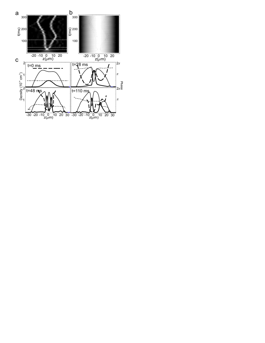
Figure 6: Strong probe case: Formation of vector solitons. Dynamics resulting from using a relatively strong probe input $\Omega_{p0}=(2\pi)~{}5.7~{}\mathrm{MHz},\,\Omega_{c0}=(2\pi)~{}8~{}\mathrm{MHz}$. In this case we have $N_{c}=0.5\times 10^{6}$ Rb-87 atoms in a $\omega_{z}=(2\pi)~{}21~{}\mathrm{Hz}$ trap and use $f_{13}=f_{23}=1/12$, and $a_{11}=a_{22}=5.36~{}\mathrm{nm}$ corresponding to the system $|1\rangle=|5S_{1/2},F=1,M_{F}=-1\rangle,\,|2\rangle=|5S_{1/2},F=1,M_{F}=+1\rangle$, and $|3\rangle=|5P_{1/2},F=2,M_{F}=0\rangle$. We artificially set $a_{12}=1.04\,a_{11}$ to exaggerate the phase separation dynamics. (a) Evolution of density in $|2\rangle$ $N_{c}|\psi_{2}(z,t)|^{2}/A$ shows the development and interaction of two vector solitons. The dotted lines indicate the times plotted in (c). (b) The total density $N_{c}(|\psi_{1}(z,t)|^{2}+|\psi_{2}(z,t)|^{2})/A=N_{c}\psi_{0}^{2}/A$ remains almost constant in time. (c) The densities $N_{c}|\psi_{1}(z,t)|^{2}/A$ and $N_{c}|\psi_{2}(z,t)|^{2}/A$ (now on the same scale) are plotted as thin and thick solid curves, respectively, at the times indicated. The phases $\phi_{1},\,\phi_{2}$ are plotted as dotted and dashed curves.

The two-component dynamics are even richer when one uses strong probe pulses so nonlinear effects become very evident in the evolution. In such a case, the qualitative features of the dynamics will be strongly effected by whether or not the relative scattering lengths are in a phase separating regime $a_{12}>\sqrt{a_{11}a_{22}}$ phaseSeperation ; phaseSeperationTh . Experiments have confirmed that the $|1\rangle,\,|2\rangle$ studied in our previous examples in Rb-87 are very slightly in the phase separating regime multipleComponentJILA . Relative scattering lengths can also be tuned via Feshbach resonances feshbach .

Figure 6 shows the evolution of the two components following the input and stopping of a stronger probe ($\Omega_{p0}=0.71\,\Omega_{c0}$). In this case we chose our levels to be $|1\rangle=|5S_{1/2},F=1,M_{F}=-1\rangle,\,|2\rangle=|5S_{1/2},F=1,M_{F}=+1\rangle$, and $|3\rangle=|5P_{1/2},F=2,M_{F}=0\rangle$, which would require an optical trap opticalTrap in order to trap the $|1\rangle$ and $|2\rangle$ equally. This level scheme is advantageous in the strong probe case since $f_{13}=f_{23}$ which, as we will discuss in more detail in Section V.3, improves the fidelity of the writing and output processes. We chose the scattering length $a_{12}=1.04\,a_{11}$, higher than the actual background scattering length, to exaggerate the phase separation dynamics. One sees in Fig. 6(a),(c) that over a 30 ms timescale, the phase separation causes the density in $|2\rangle$ to become highly localized and dense. This occurs because the scattering length $a_{12}>a_{11}$ causes $|1\rangle$ atoms to be repelled from the region occupied by the $|2\rangle$ atoms, and in turn the $|2\rangle$ atoms find it favorable to occupy the resulting “well” in the $|1\rangle$ density. These two processes enhance each other until they are balanced by the cost of the kinetic energy associated with the increasingly large spatial derivatives and we see the formation of two-component (vector) solitons twoCompSolitons . In the case here, two solitons form and propagate around the BEC, even interacting with each other. The alternating grey and white regions along each strip in Fig. 6(a) indicate that the solitons are undergoing breathing motion on top of motion of their centers of mass. Fig. 6(b) shows that the total density profile $\psi_{0}^{2}$ varies very little in time. It is the relative densities of the two components that accounts for nearly all the dynamics.

We found solitons formed even in only slightly phase separating regimes ($a_{12}/\sqrt{a_{11}a_{22}}\geq 1.02$). The number of solitons formed, the speed of their formation, and their width were highly dependent on this ratio as well as the number of atoms in $|2\rangle$. The ability of stopped light pulses to create very localized two-component structures seems to be a very effective method for inducing the formation of vector solitons, which has hitherto been unobserved in atomic BECs. A full exploration of these dynamics is beyond our scope here.

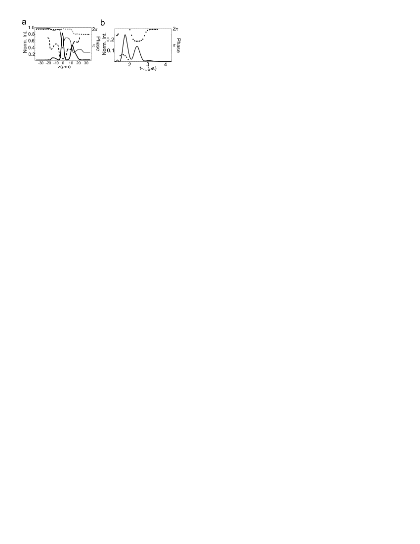
Figure 7: Writing solitons onto probe field. (a) Writing of vector solitons onto probe and coupling fields directly after a switch-on after a storage time of $\tau_{\mathrm{st}}=110~{}\mathrm{ms}$ and (b) probe output. The plots use the same conventions as Fig. 5(d-e).

These non-trivial features can also be written onto probe pulses as shown in Fig. 7(a). Note that the condition for coherent revivals $|\alpha_{NA}|\ll\alpha_{A}$ does not depend on the weak probe limit. Therefore, the writing process is still primarily a coherent process, and (18) is still well satisfied. However, we see in Fig. 7(a), the coupling field is strongly affected by the writing and is far from homogenous, meaning the weak probe result (19) can not be used. Nonetheless, we see that the qualitative features of both the density and phase of $\psi_{2}$ have still been transferred onto $\Omega_{p}$. The writing in the strong probe regime will be studied in more detail in Section V.

In Fig. 7(b) we plot the resulting output probe pulse in this case. As in the weak probe case there is some degradation in the subsequent propagation due to attenuation of high frequency components. In addition, unlike the weak probe case, there are nonlinearities in the pulse propagation itself which causes some additional distortion. Section V.3 also addresses this issue. Even so, we again see a very clear signature of the two solitons in the both the intensity and phase of the output probe.

We have performed some preliminary simulations in traps with weaker transverse confinement and which calculate the evolution in the transverse degrees of freedom. They show that the solitons can break up into two-component vortex patterns via the snake instability snake ; SolitonVortex .

We chose our parameters to be in the phase separating regime here. Just as in the weak probe case, other regimes will lead instead to much gentler dynamics. For example, it has been shown breatheTogether that when $a_{12}<a_{11}=a_{22}$ then there exist “breathe-together” solutions of the BEC whereby complete overlap of the wavefunctions $\psi_{1},\psi_{2}$ persists. In this case the nonlinear atomic interaction can lead to spin-squeezing spinSqueezing . It would be extremely interesting to investigate a probe-revival experiment in such a case, to see to what extent the squeezed statistics are written into probe pulse, producing squeezed light squeezedLight . This would require taking both the light propagation and atomic dynamics in our formalism beyond the mean field. Steps in this direction have been taken in quantumProcessing ; squeezedLightRaman , but these analyses are restricted to the weak probe case.

V Quantitative study of writing and output

The above examples demonstrate that a rich variety of two component BEC dynamics can occur, depending on the relative interaction strengths and densities of the states involved. They also show that remarkably complicated spatial features in both the density and phase can be written into temporal features of a probe light pulse and output. The purpose of this section is to quantify the fidelity with which wavefunctions can be written onto the probe field.

To do this we consider an example of a two-component BEC with a Gaussian shaped feature in $\psi_{2}$, with parameters characterizing length scales and amplitudes of density and phase variations. Note these Gaussian pulse shapes are relevant to cases in which one might perform controlled processing, e.g. Fig. 5. Switching on a coupling field then generates and outputs a probe pulse with these density and phase features. We will calculate this output, varying the parameters over a wide range. In each case, we will compare the output to what one expect from an “ideal” output (without dissipation or distortion), and calculate an error which characterizes how much they differ. Using the analysis of the switching process in Section III and the USL propagation in Section II we also obtain analytic estimates of this error.

In the weak probe case, we find a simple relationship between $\psi_{2}(z,t_{\mathrm{on}})$ and the output $\Omega_{p}^{(\mathrm{out})}(t)$. We find that to optimize the fidelity in this case one should choose the Gaussian pulse length between two important length scales. The shorter length scale is determined by EIT bandwidth considerations, which primarily contribute error during the output. On the other hand, for large pulses comparable to the total condensate size, the error during the writing process dominates due to $\psi_{2}$ partially occupying the condensate entering edge region ($z<z_{c}$).

In the strong probe case, we find that the relationship between $\psi_{2}(z,t_{\mathrm{on}})$ and $\Omega_{p}^{(\mathrm{out})}(t)$ is more complicated, however, when $f_{13}=f_{23}$, one can still make an accurate correspondence. We find the fidelity in this case depends only weakly on the probe strength. Conversely, when $f_{13}\not=f_{23}$, even a small nonlinearity causes additional phase shifts and distortions, making this correspondence much more difficult, leading to higher errors for stronger probes. For this reason, a system that uses, for example $|1\rangle=|F=1,M_{F}=-1\rangle,\,|2\rangle=|F=1,M_{F}=+1\rangle$ (as in Fig. 7) would be preferable when one is interested in applications where there are comparable densities in the two states.

By considering the switch-on and output processes, starting with an arbitrary initial two-component BEC, we emphasize that this method of outputting the atomic field information onto light fields works regardless of how the BEC state was generated. One could prepare a BEC in a coherent superposition of $|1\rangle$ and $|2\rangle$ by any available method including, but not limited to, inputting a slow light pulse.

V.1 Deriving $\psi_{2}$ from the written and output probe field.

Assume we have a two component BEC with wavefunctions $\psi_{1},\psi_{2}$ (and again define $\psi_{0}\equiv\sqrt{|\psi_{1}|^{2}+|\psi_{2}|^{2}}$). For now we assume $f_{13}=f_{23}$ (so $\alpha_{12}=0$, see Eq. (III.1)), as we treat the $f_{13}\not=f_{23}$ case in Section V.3. Upon a rapid switch-on of a coupling field with amplitude $\Omega_{c0}$, inverting (12) shows the pattern written onto the probe field will be:

$$\Omega_{p}^{\mathrm{(rev)}}=-\frac{\psi_{2}}{\psi_{0}}\Omega_{D}+\frac{\psi_{1}^{*}}{\psi_{0}}\Omega_{A}$$ (22)

In the ideal limit, where the spatial variations of the wavefunction are sufficiently small, $\alpha_{NA}\rightarrow 0$ and the second term vanishes. Furthermore, (17) shows in this case that the dark field intensity is constant $|\Omega_{D}|=\Omega_{c0}$. So in the ideal limit we have for the amplitude:

$$|\Omega_{p}^{({\mathrm{rev-ideal}})}|=\frac{|\psi_{2}|}{\psi_{0}}\Omega_{c0}$$ (23)

In practice this will be a good approximation so long as the inequality $|\alpha_{NA}||\psi_{1}|\ll\alpha_{A}|\psi_{2}|$ is satisfied. The extent to which the second term in (22) cannot be neglected will determine the error between the ideal $\Omega_{p}^{({\mathrm{rev-ideal}})}$ and actual $\Omega_{p}^{({\mathrm{rev}})}$ output. Note that in all the cases studied in Section IV, $\psi_{0}(z,t)$ was nearly constant in time, being always well approximated by the original ground state $\psi_{1}^{\mathrm{(G)}}(z)$. Thus $\psi_{0}$ can be considered a known function of $z$.

Turning now to the phase, the simple relationship $\phi_{2}-\phi_{1}=\phi_{p}-\phi_{c}+\pi$ is always satisfied in the dark state (see (18)). If $\phi_{c}$ was just a constant then the probe phase would simply reflect the relative phase of the two wavefunctions $\phi_{p}=\phi_{2}-\phi_{1}+\pi$ (choosing our phase conventions so $\phi_{c}=0$). This is indeed the case in the weak probe limit, as then the coupling field phase $\phi_{c}$ is unaffected by the atomic fields upon the switch-on. However, this is not necessarily so in the strong probe regime. To calculate the true phase shift, we calculate phase of $\Omega_{D}$ from (17). In the ideal limit $\phi_{D}(z)=\int_{z_{\mathrm{in}}}^{z}dz^{\prime}\alpha_{l}(z^{\prime})$ (choosing our phase conventions such that $\phi_{1}(z_{\mathrm{in}})=0$). Defining $\phi_{21}\equiv\phi_{2}-\phi_{1}$ and using the definition of $\alpha_{l}$ (III.1) and (23), we find the relationship:

$$\phi_{21}(z) = \phi_{p}^{({\mathrm{rev-ideal}})}(z)+\pi-\phi_{p}^{(\mathrm{nl})};$$

$$\phi_{p}^{(\mathrm{nl})} = \int_{z_{\mathrm{in}}}^{z}dz^{\prime}\frac{d\phi_{p}^{({\mathrm{rev-ideal}})}}{dz^{\prime}}\frac{|\Omega_{p}^{({\mathrm{rev-ideal}})}(z^{\prime})|^{2}}{\Omega_{c0}^{2}-|\Omega_{p}^{({\mathrm{rev-ideal}})}(z^{\prime})|^{2}},$$

The equation is written in this way (the atomic phase in terms of the probe phase and intensity) because our purpose is to derive the phase pattern $\phi_{21}$ based on the observed probe field, rather than vice versa. The nonlinear correction $\phi_{p}^{(\mathrm{nl})}$ is fact the phase imprinted on the coupling field $\phi_{c}$ during the switch-on.

However, in an experiment, we do not have direct access to the revived probe $\Omega_{p}^{\mathrm{(rev)}}(z)$. Rather, we observe the temporal output $\Omega_{p}^{\mathrm{(out)}}(t)$. In practice, the intensity of this quantity can be measured with a PMT, while the phase pattern could be measured by beating it with a reference probe field which did not propagate though the BEC. In the ideal limit (the absence of attenuation or distortion) the relationship (20) will link the observed output to the revived probe field $\Omega_{p}^{\mathrm{(rev)}}$. Thus we define the “ideal” output via

$$\Omega_{p}^{(\mathrm{rev-ideal})}(z)\equiv\Omega_{p}^{(\mathrm{out-ideal})}\big{(}\tau(z_{\mathrm{out}})-\tau(z)+t_{\mathrm{on}}\big{)}$$ (25)

In practice, additional absorption events and distortion can occur during the output. If variations of the relative amplitude $\psi_{2}/\psi_{1}$ have some characteristic scale $L_{\psi}$ then time features with a scale $\tau\sim L_{\psi}/V_{g}$ will be introduced into the probe $\Omega_{p}$. Using our result for the bandwidth induced attenuation (5) yields an estimate for transmission energy (that is, the energy of the actual output pulse $\Omega_{p}^{(\mathrm{out})}$ relative to an unattenuated output of $\Omega_{p}^{(\mathrm{rev})}$):

$$T = \frac{1}{\sqrt{1+\beta}};$$

$$\beta \equiv \frac{D(z_{\mathrm{out}})-D(z_{\mathrm{p}})}{\big{(}L_{\psi}\alpha_{A}(z_{\mathrm{p}})\big{)}^{2}}$$ (26)

For this simple estimate we evaluate $\alpha_{A}$ and $D$ at the location of the center of the pulse $z_{p}$, though one could also construct more sophisticated estimates by integrating over the spatial distribution of the pulse. Just as in our discussion below Eq. (5), the temporal width is increased by a factor $T^{-1}$ and the peak intensity reduced by $T^{2}$ during the propagation out.

We now apply these findings to a Gaussian pulse, with $\psi_{2}$ assumed to be of the form,

$$\psi_{2}(z)=\psi_{0}(z)A_{2}\,\mathrm{exp}\bigg{(}-\frac{z^{2}}{2L_{2}^{2}}\bigg{)}\mathrm{exp}\bigg{[}i\frac{A_{\phi_{2}}}{2}\mathrm{erf}\bigg{(}\frac{z}{L_{\phi_{2}}}\bigg{)}\bigg{]}$$ (27)

Note $\psi_{2}$ has a density feature of amplitude $A_{2}^{2}$ and length $L_{2}$ and a phase feature of amplitude $A_{\phi_{2}}$ and length $L_{\phi_{2}}$. For $\psi_{1}(z)$ we choose the amplitude so the total density matches the ground state for the trap $\psi_{0}^{2}=|\psi_{1}^{(\mathrm{G})}|^{2}$ and in the phase we put in a shift with some amplitude $A_{\phi_{1}}$ and length $L_{\phi_{1}}$. An example is shown in Fig. 8(a). These parameters will be varied throughout this section to learn how they effect the writing and output. We choose a $\omega_{z}=(2\pi)~{}20~{}$Hz trap ($A=\pi(5~{}\mu\mathrm{m})^{2}$) with $N_{c}=2.0\times 10^{6}$ Rb-87 atoms. We use $f_{13}=f_{23}=1/12$, corresponding to the system $|1\rangle=|5S_{1/2},F=1,M_{F}=-1\rangle,\,|2\rangle=|5S_{1/2},F=1,M_{F}=+1\rangle$, and $|3\rangle=|5P_{1/2},F=2,M_{F}=0\rangle$ in Rb-87.

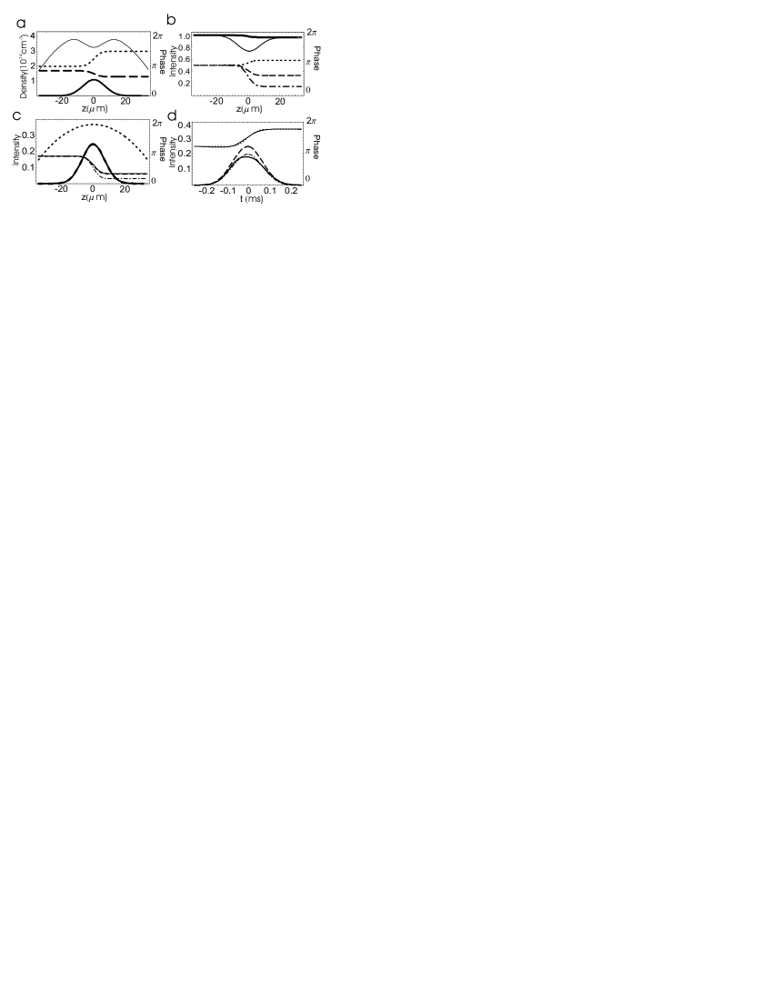
Figure 8: Writing and outputting atomic field information onto the probe fields. (a) A test case with a density feature of length $L_{2}=10~{}\mu\mathrm{m}$ of amplitude $A_{2}=0.5$ and phase features of $A_{\phi_{2}}=-0.2\,\pi,\,L_{\phi_{2}}=5~{}\mu\mathrm{m}$ (see Eq. (27)) and $A_{\phi_{1}}=0.5\,\pi,\,L_{\phi_{1}}=5~{}\mu\mathrm{m}$. The conventions for the curves are the same as Fig. 6(c). (b) Upon switch-on of the coupling field with $\Omega_{c0}=(2\pi)~{}8~{}$MHz, we show the dark intensity $|\Omega_{D}(z)/\Omega_{c0}|^{2}$ (thick solid curve) and coupling intensity $|\Omega_{c}(z)/\Omega_{c0}|^{2}$ (thin solid). The dotted, dashed, and dot-dashed curves show, respectively, the phase profiles $\phi_{c}$, $\phi_{D}$ and $\phi_{21}$. (c) The normalized probe intensity profile $|\Omega_{p}^{\mathrm{(rev)}}|^{2}/\Omega_{c0}^{2}$ (solid curve) is indistinguishable from the expected profile $|\Omega_{p}^{\mathrm{(rev-ideal)}}|^{2}/\Omega_{c0}^{2}$ (thick dashed) (see Eq. (23)). The thin solid curve shows $\phi_{p}^{\mathrm{(rev)}}$ and the dot-dashed curve shows $\phi_{21}+\pi$, while the thin dashed curve shows the expected probe phase profile with the nonlinear correction $\phi_{p}^{\mathrm{(rev-ideal)}}=\phi_{21}+\phi_{p}^{\mathrm{(nl)}}+\pi$ (V.1). For reference, the dotted curve shows the total density $\psi_{0}^{2}$ profile. (d) The temporal pattern of the output probe intensity $|\Omega_{p}^{\mathrm{(out)}}|^{2}/\Omega_{c0}^{2}$ (thick solid curve) and phase $\phi_{p}^{\mathrm{(out)}}$ (thin solid), versus an estimate based on perfect propagation of the revived pulse $\Omega_{p}^{\mathrm{(rev)}}$ according to (20) (dashed and dotted curves). The dot-dashed curve shows the ideal output attenuated by $T^{2}$ (see (V.1) and the discussion afterward) using the estimate $L_{\psi}=(L_{2}^{-2}+A_{\phi_{2}}L_{\phi_{2}}^{-2}+A_{\phi_{1}}L_{\phi_{1}}^{-2})^{-1/2}$.

In the example of Fig. 8(a), $A_{2}=0.5$ is not particularly small, so the weak probe limit can not be assumed. Figure 8(b) shows the spatial profiles of the dark field $\Omega_{D}$ and coupling field $\Omega_{c}$ immediately following a fast switch-on ($\tau_{s}=0.1~{}\mu\mathrm{s}$). We see very little attenuation of $\Omega_{D}$ occurs across the BEC, as $\alpha_{NA}\sim\mathcal{O}(A_{2}L_{2},iA_{2}A_{\phi_{2}}L_{\phi_{2}},iA_{2}A_{\phi_{1}}L_{\phi_{1}})$ is quite small compared with $\alpha_{A}$. Translating this back into the $\Omega_{c},\Omega_{p}$ basis, (12) predicts that $\Omega_{c}$ acquires a dip in intensity with a height proportional to the density $|\psi_{2}|^{2}$. This behavior is indeed seen in the figure.

The phase difference $\phi_{21}$ is plotted as the dot-dashed curve in Figure 8(b). One sees that in the region where $\phi_{21}$ is inhomogeneous, a small phase shift, equal to $\phi_{p}^{(\mathrm{nl})}$ (V.1), is introduced in the coupling field (dotted curve). Again this shift only arises in the strong probe regime. The phase shift in the dark field $\phi_{D}$ is plotted as the dashed curve.

Figure 8(c) then compares written probe field to our ideal limit predictions (23)-(V.1) in this example. The numerically calculated intensity $|\Omega_{p}^{({\mathrm{rev}})}|^{2}$ (solid curve) is almost indistinguishable from our prediction $|\Omega_{p}^{({\mathrm{rev-ideal}})}|^{2}$ (23) (dashed curve). The phase written onto the probe field $\phi_{p}^{({\mathrm{rev}})}$ is also very close to the ideal limit prediction (V.1). One sees that including the nonlinear correction $\phi_{p}^{\mathrm{(nl)}}$ to the simpler estimate $\phi_{21}+\pi$ (dot-dashed curve) is important in making the comparison good.

Figure 8(d) then shows intensity (thick solid curve) and phase (thin solid) of the output pulse $\Omega_{p}^{({\mathrm{out}})}(t)$. For comparison the dashed and dotted curves show, respectively, the output expected from an unattenuated and undistorted transmission of the revived pulse $\Omega_{p}^{({\mathrm{rev}})}(z)$ via (25). One sees a very good agreement in the phase pattern, while there is a visible reduction in the intensity, due to bandwidth considerations. The dot-dashed curve shows the our estimate with the estimated reduction in intensity $T^{2}$ (see (V.1)) using a characteristic length scale $L_{\psi}$ calculated from a quadrature sum of contributions from the amplitude and phase features in (27) (the expression is given in the caption).

We have thus calculated a method by which the output probe pulse can be solely used to calculate the relative density and phase of the wavefunctions which generated it, and demonstrated the method with a generic example. Furthermore, we have identified the leading order terms which will cause errors in these predictions. In particular we have seen in our example in Fig. 8(d) that including the expected bandwidth attenuation accounts for most of the deviation between our ideal predictions and the actual output pulse.

V.2 Quantifying and estimating the fidelity.

We now quantify the deviations from our predictions (23-25) for our example (27), varying the length and amplitude parameters over a wide range. These results can be directly applied to pulses which are approximately Gaussian (as in Fig. 5). The results here should also provide a good guide to the expected fidelity in more complicated cases so long as the length scale and amplitude of features can be reasonably estimated.

To quantify the deviation from our ideal case prediction (23)-(V.1) we define the write error:

$$E_{w}\equiv\frac{\int_{z_{\mathrm{in}}}^{z_{\mathrm{out}}}\,dz^{\prime}\bigg{|}\,\Omega_{p}^{(\mathrm{rev})}-|\Omega_{p}^{(\mathrm{rev-ideal})}|e^{i(\phi_{21}+\phi_{p}^{\mathrm{(nl)}}+\pi)}\bigg{|}^{2}}{\int_{z_{\mathrm{in}}}^{z_{\mathrm{out}}}\,dz^{\prime}|\Omega_{p}^{(\mathrm{rev})}|^{2}}$$ (28)

We plot this quantity in a series of cases with different $L_{2}$ in Fig. 9(a) (circles) in a case with amplitude $A_{2}=0.5$ and no phase profiles. This is compared with a calculated prediction for $E_{w}$ (solid curve) based on (22) where we calculate $\Omega_{A}$ with (16) and calculate the small attenuation of $\Omega_{D}$ with (17). These errors grow as $L_{2}$ becomes comparable to $\alpha_{A}^{-1}=0.2~{}\mu\mathrm{m}$, according to the discussion in Section III.1. We see the agreement between the analytic and numerical estimates is quite good for small to moderate $L_{2}$, confirming that this is the leading source of error. However, when $L_{2}$ becomes comparable to the total BEC size (the Thomas-Fermi radius is $R_{z}=44~{}\mu\mathrm{m}$ here), we begin to see additional errors because $\psi_{2}$ becomes non-zero at the BEC edge. Thus, we see that for a given BEC length and density, one must choose $\alpha_{A}^{-1}\ll L_{2}\ll R_{z}$ to minimize the write error $E_{w}$. Because this edge effect depends on the density structure near the BEC edge, it is difficult to estimate analytically, but it is related to the fraction of the pulse in or near the region $z<z_{c}$. For pulses near the BEC center, this will depend on $L_{2}/R_{z}$, whereas for pulses far off center, it will also depend on the location of the center of the pulse.

We also plot a series of cases keeping $L_{2}=10~{}\mu\mathrm{m}$ and $A_{2}=0.1$ but varying the length scale $L_{\phi_{2}}$ of a phase profile of amplitude $A_{\phi_{2}}=0.75\,\pi$. One sees similar but slightly smaller errors $E_{w}$ in this case.

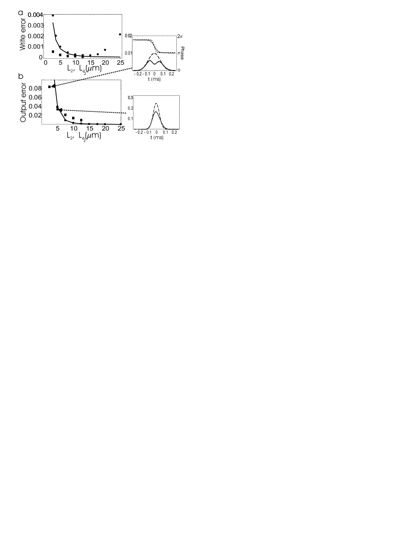
Figure 9: Writing and outputting atomic field information onto light fields. (a) Circles show the write error $E_{w}$ (28) versus the length $L_{2}$ for BECs with no phase jumps ($A_{\phi_{2}}=A_{\phi_{1}}=0$) and with $A_{2}=0.5$ (see Eq. (27)). The solid curve shows an analytic result based on the analytic expressions (22), (16) and (17). The squares show a case holding $L_{2}=10~{}\mu\mathrm{m},A_{2}=0.1$ and introducing a phase feature $A_{\phi_{2}}=0.75\,\pi$ with varying length scale $L_{\phi_{2}}$. (b) The output error $E_{\mathrm{out}}$ (29) for the same cases as (a). The solid curves showing the prediction $(5/16)\beta^{2}$ discussed in the text (choosing $L_{\psi}=L_{2}$) for the case with no phase jumps (circles). The insets show the output in the cases indicated with arrows, with the same plotting conventions as Fig. 8(d) (in the lower inset on the right $\phi_{p}$ is homogenous and not plotted), we again use $\omega_{z}=(2\pi)~{}20~{}$Hz, $A=\pi(5~{}\mu\mathrm{m})^{2}$, $N_{c}=2.0\times 10^{6}$ and $f_{13}=f_{23}=1/12$, corresponding to the system $|1\rangle=|5S_{1/2},F=1,M_{F}=-1\rangle,\,|2\rangle=|5S_{1/2},F=1,M_{F}=+1\rangle$, and $|3\rangle=|5P_{1/2},F=2,M_{F}=0\rangle$ in Rb-87.

We define the error accumulated as $\Omega_{p}^{\mathrm{(rev)}}$ propagates out using (20):

$$E_{\mathrm{out}}\equiv\frac{\int_{z_{\mathrm{in}}}^{z_{\mathrm{out}}}\,dz^{\prime}|\Omega_{p}^{(\mathrm{rev})}(z^{\prime})-\Omega_{p}^{(\mathrm{out})}\big{(}\tau(z_{\mathrm{out}})-\tau(z^{\prime})\big{)}|^{2}}{\int_{z_{\mathrm{in}}}^{z_{\mathrm{out}}}\,dz^{\prime}|\Omega_{p}^{\mathrm{(rev)}}(z^{\prime})|^{2}}$$ (29)

In Fig. 9(b) we plot this quantity for the cases corresponding to Fig. 9(a). For comparison, for the series with no phase shift, we calculated an estimate based on the expected attenuation $T^{2}$ and spreading $T^{-1}$ of a Gaussian pulse, due bandwidth considerations (see Eq. (V.1) and subsequent discussion), choosing $L_{\psi}=L_{2}$. In the limit of small $\beta$ this calculation yields $E_{\mathrm{out}}\approx(5/16)\beta^{2}$. This is plotted as a solid curve and we see good agreement with the numerical data.

The error $E_{\mathrm{out}}$ is seen to dominate $E_{w}$ for small $L_{2}$, due to the fact that the large optical density effects the former ($D(z_{\mathrm{out}})=617$ in the case plotted). Thus our analytic estimate $E_{\mathrm{out}}=(5/16)\beta^{2}$ is a good estimate of the total error. But for larger $L_{2}$ the edge effect in $E_{w}$ becomes important. To minimize the total error $E_{w}+E_{\mathrm{out}}$ we should choose $L_{2}$ so the error $E_{\mathrm{out}}=(5/16)\beta^{2}$ is comparable to the edge effect error. In Fig. 9 the optimal length is $L_{2}^{\mathrm{(opt)}}\approx 17.5~{}\mu\mathrm{m}$ and the total error is $E_{\mathrm{out}}+E_{w}\approx 0.0009$. The scaling of $L_{2}^{\mathrm{(opt)}}$ with the condensate size $R_{z}$ is difficult to estimate. Assuming it roughly increases as $L_{2}^{\mathrm{(opt)}}\propto R_{z}$, then (V.1) shows $\beta^{\mathrm{(opt)}}\propto 1/D(z_{\mathrm{out}})$, giving us a guide as to the improvement in fidelity we can expect by increasing the total optical density of the condensate.

The insets show the plots of the ideal output of $\Omega_{p}^{\mathrm{(rev)}}(z)$ (solid curves) versus actual outputs $\Omega_{p}^{\mathrm{(out)}}(t)$ (dotted curves) in two of the cases. In one case, with no phase jumps and a small $L_{2}$, we see an overall reduction in amplitude and slight spreading. In the other, with a larger $L_{2}$ but a phase shift with a small length scale $L_{\phi_{2}}$, we see that the attenuation is localized in the middle of the pulse. This is because it is the components which contain the sharpest phase profile, near the middle, which are most severely attenuated. Generally, in cases with complicated spatial features, one must be aware of this potential for local attenuation of the sharpest features. Note, however, that in many cases of interest, such as the interference fringes (Fig. 4) and solitons (Fig. 6), large phase shifts occur primarily in regions of low density, meaning these features often survive during the output propagation.

Figure 10: Writing and outputting atomic field information onto light fields. (a) The write error $E_{w}$ (28) versus $A_{2}$ for the case $L_{2}=10~{}\mu\mathrm{m},\,L_{\phi_{1}}=L_{\phi_{2}}=5~{}\mu\mathrm{m},\,A_{\phi_{1}}=0.5\pi,\,A_{\phi_{2}}=0.2\pi$. (b) The output error $E_{\mathrm{out}}$ (29) in the same cases. The solid line shows the estimate $(5/16)\beta^{2}$ (see Eq. (V.1)) using $L_{\psi}=(L_{2}^{-2}+A_{\phi_{2}}L_{\phi_{2}}^{-2}+A_{\phi_{1}}L_{\phi_{1}}^{-2})^{-1/2}$. The condensate parameters are the same as in Fig. 9.

Our analysis of switching process in Section III applies even with a large amplitude $A_{2}$, as was seen in the $A_{2}=0.5$ case in Fig. 8. In Fig. 10(a) we plot the results of a series of simulations with $A_{2}$ varying all the way up to $A=0.9$ and see only a very small impact on $E_{w}$ for $A_{2}\leq 0.8$. Most of our results for the propagation of USL pulses, e.g. (4) and (5), rely on the weak probe limit. Surprisingly though Fig. 10(b) shows that the output error $E_{\mathrm{out}}$ is independent of $A_{2}$ through $A_{2}=0.9$.

V.3 Effect of unequal oscillator strengths

The lack of distortion in the strong probe cases discussed so far in this section is a result of us choosing a system with equal oscillator strengths $f_{13}=f_{23}$. The importance of the relative size of the oscillator strengths can be understood by considering the adiabatons (the changes in the output coupling intensity seen in Fig. 2(a,e)). The adiabatons arise because of the coherent flow of photons between the two light fields and their amplitude is determined by the requirement that the sum of the number of photons in both fields is constant upon such an exchange. In a case where $\Omega_{p}\sim\Omega_{c}$ one must take into account that it is the total field strength $|\Omega|^{2}=|\Omega_{p}|^{2}+|\Omega_{c}|^{2}$, rather than simply the input coupling strength $\Omega_{c0}^{2}$ which enters the numerator in our equation for the group velocity $V_{g}(z)$ (4). However, the expressions for the Rabi frequencies involve the oscillator strengths of the relevant transitions. Thus, preserving the total number of photons at each point in space will result in a homogenous $|\Omega|^{2}=\Omega_{c0}^{2}$ if and only if $f_{13}=f_{23}$. During the time that the probe is completely contained in the BEC, $|\Omega|^{2}$ will differ from $\Omega_{c0}^{2}$ in the vicinity of the pulse according to:

$$|\Omega(z,t)|^{2}=\Omega_{c0}^{2}+|\Omega_{p}(z,t)|^{2}\bigg{(}1-\frac{f_{23}}{f_{13}}\bigg{)}$$ (30)

This leads to a nonlinear distortion, whereby the center of the pulse (where the probe intensity is greatest) tends to move faster or slower than the front and back edges, depending on the sign of term in parentheses. This behavior is quite clearly seen in Fig. 11, where we compare a delayed weak probe regular USL output pulse to cases with strong probes $\Omega_{p0}=\Omega_{c0}$ and vary $f_{23}=1/3,1/2,2/3$ ($f_{13}=1/2$ in all cases). Each time we chose the coupling intensity so that that the Rabi frequency is $\Omega_{c0}=(2\pi)~{}8~{}\mathrm{MHz}$. One sees that when $f_{13}=f_{23}$ there is no asymmetrical distortion, though we get a slight spreading and a shorter delay time. However, in the other two cases, there is asymmetry in the output pulses, consistent with the picture that the center of the pulse will travel slower or faster than the edges according to (30) and (4) (with $\Omega_{c0}^{2}$ replaced by $|\Omega|^{2}$ in the numerator). The result is a breakdown of our estimate (25). As this is a propagation effect, the absolute magnitude of this effect should roughly be linear with optical density and the relative distortion will go as the optical density divided by the pulse length. This is the primary reason it would be advantageous to use the levels we chose in our simulation in Fig. 7 if there is a strong probe.

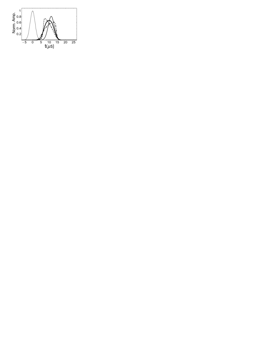
Figure 11: USL with a strong probe. The dotted curve shows a strong probe pulse amplitude with peak value $\Omega_{p0}=\Omega_{c0}=(2\pi)~{}8~{}\mathrm{MHz}$ input into a sodium cloud with an optical density $D(z_{\mathrm{out}})=407$. We use an oscillator strength $f_{13}=1/2$ but vary the coupling oscillator strength $f_{23}$. The output $\Omega_{p}^{\mathrm{(out)}}/\Omega_{p0}$ is shown in the cases $f_{23}=1/2$ (thick solid curve), $f_{23}=2/3$ (dot-dashed curve), and $f_{23}=1/3$ (dashed curve). For reference, the thin solid curve shows output for a weak input probe $\Omega_{p0}=(2\pi)~{}1.4~{}\mathrm{MHz}$.

We just outlined the reason that the equal oscillator strengths can be important in reducing distortion during propagation and thus $E_{\mathrm{out}}$. It turns out that the writing process is also more robust when $f_{13}=f_{23}$. The reason is the presence of the additional term $\alpha_{12}$ (III.1). This term is quite small in the weak probe limit, but in the strong probe case leads to an additional phase shift, not accounted for in (V.1), which depends in detail on the pulse amplitude and structure.

Figs. 12(a-d) shows a case, similar to Fig. 8, but with $f_{13}=1/12,f_{23}=1/4$ (as in the cases in Figs. 4-5), and with a fairly small nonlinearity $A_{2}=0.25$. One sees in Fig. 12(b) that there is a dip in $\Omega_{D}$ in the region of the probe due to the $\alpha_{12}$ term. Fig. 12(c) shows the written probe pulse. There is a small but discernable difference between the predicted $\phi_{p}^{\mathrm{(rev-ideal)}}$ (V.1) and actual $\phi_{p}^{\mathrm{(rev)}}$ phase. Fig. 12(d) then shows the asymmetric distortion which develops as the strong probe propagates out. One sees the phase jump is distorted in addition to the amplitude. Figs. 12(e-f) demonstrate how these effects lead to substantially higher errors $E_{w}$ and $E_{\mathrm{out}}$ as $A_{2}$ becomes larger. From our estimate from the previous section we expect an output error of $E_{\mathrm{out}}=0.0147$ and we see in Fig. 12(f) that the distortion effect leads to errors higher than this when $A_{2}\geq 0.3$.

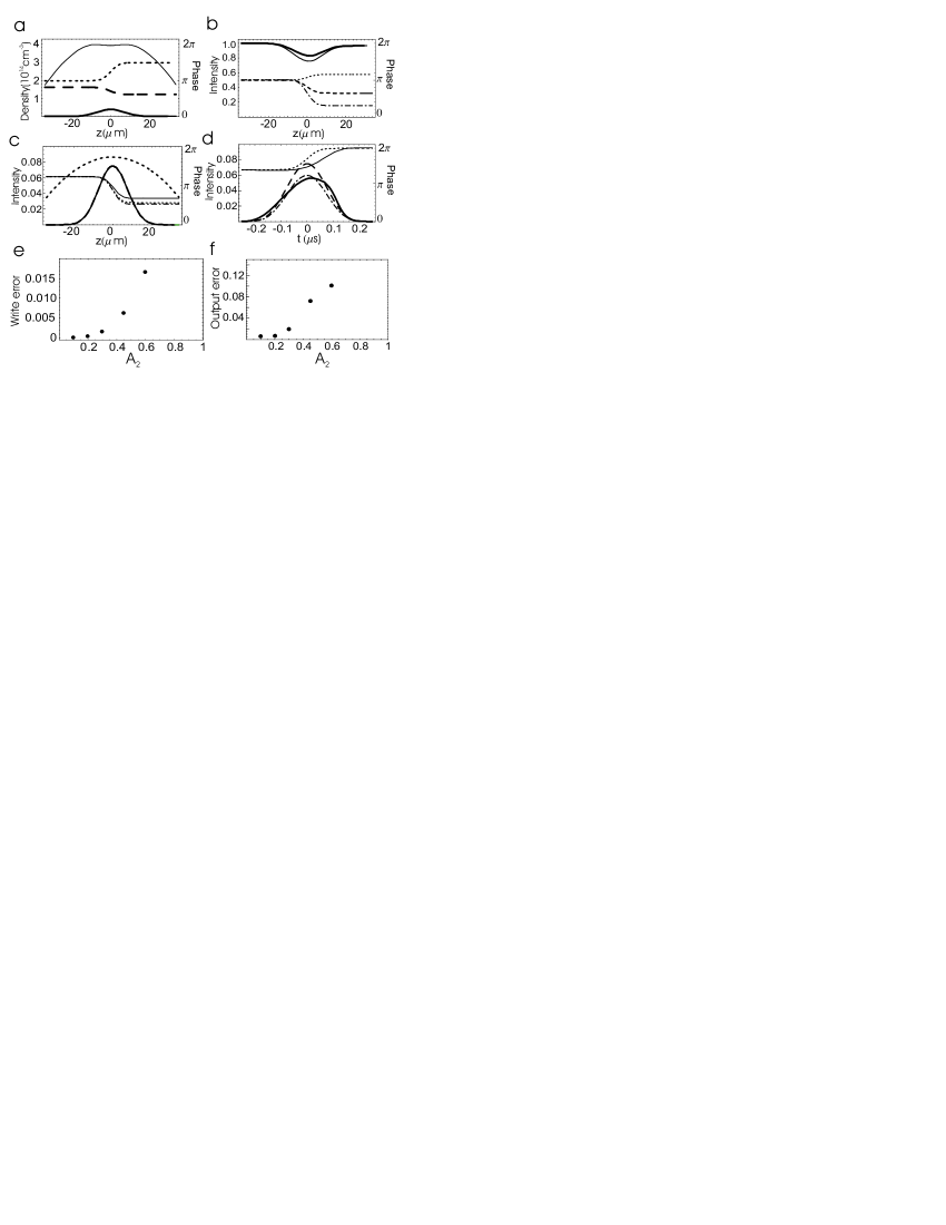
Figure 12: Writing information with unequal oscillator strengths. (a-d) Plots are for the same parameters as Fig. 8 except with $f_{12}=1/12,\,f_{23}=1/4$ and $A_{2}=0.25$. (e-f) Write $E_{w}$ and output $E_{\mathrm{out}}$ errors versus $A_{2}$ for the parameters $L_{2}=10~{}\mu\mathrm{m},\,L_{\phi_{1}}=L_{\phi_{2}}=5~{}\mu\mathrm{m},\,A_{\phi_{1}}=0.5\,\pi,\,A_{\phi_{2}}=-0.2\,\pi$.

We thus conclude that fidelity of both the writing and output is compromised in a system with unequal oscillator strengths. However, this only comes into effect in cases where the nonlinearity is important. In weak probe cases neither of these effects is important and the fidelity can still be estimated with the analysis of the $f_{13}=f_{23}$ case in Sections V.1-V.2.

VI Outlook

In conclusion, we have established first several new results regarding the fast switching of the coupling field in light storage experiments. We found the switching could be done arbitrarily fast without inducing absorptions so long as the probe is completely contained in the atomic medium (and $V_{g}\ll c$ which is usually the case in practice). We have also seen that when the switching is slow compared to the excited state lifetime ($\sim 25$ ns), the probe smoothly follows the temporal switching of the coupling field, while in the other limit the probe amplitude undergoes oscillations which damp out with this time scale (see Fig. 3).

Next, we saw that these stopped pulses can induce novel and rich two-component BECs dynamics during the storage time. Both the relative scattering lengths of the states used and the probe to coupling intensity ratio have a strong effect on the qualitative features of the dynamics. In the weak probe case, the $|2\rangle$ condensate sees en either an effective repulsive hill (when $a_{12}>a_{11}$, see Fig.4(b)) or harmonic oscillator potential (when $a_{12}<a_{11}$, see Fig.5(a)). The characteristic timescale for the dynamics is given my the chemical potential of the BEC (in our cases $\sim(2\pi)~{}1~{}$kHz) times the relative scattering length difference $|a_{12}-a_{11}|/a_{11}$. In the latter case, the resulting evolution can be easily calculated by decomposing the pulse into the various harmonic oscillator eigenstates. Thus it is possible to choose input pulses which preserve their density over time or undergo predictable reshaping such as dipole sloshing or breathing, allowing controlled storage and linear processing of optical information. Inputting stronger probes will add nonlinearity to the evolution, making nonlinear processing possible. Very strong probes and phase separating scattering lengths $a_{12}^{2}>a_{11}a_{22}$ lead to the formation and motion of vector solitons, which have not been observed in BECs to date.

We then showed that switching the coupling field on after the dynamics writes the various density and phase features of the wavefunctions onto revived probe pulses. This was seen qualitatively for various examples (Figs. 4-7). A precise relationship between the wavefunctions and output pulses was found (23)-(25), meaning the output probe pulse can be used as a diagnostic of the relative density and phase in the BEC wavefunctions. We have also identified sources of attenuation and distortion in the writing and output processes and quantitative errors were calculated for a wide range of length and amplitudes of Gaussian pulses (Figs. 9-10). As we saw there, the error during the output dominates for shorter pulses and is $(5/16)\beta^{2}$ (see Eq. (V.1)). For longer pulses effects due to the condensate edge introduce errors into the writing process. Balancing these two considerations one can optimize the fidelity, which improves with optical density.

For the strong probe case, we found that for equal oscillator strengths ($f_{13}=f_{23}$), one could still relate the wavefunctions to the output pulses by taking into account an additional nonlinear phase shift (V.1). The fidelity of transfer of information was virtually independent of the probe strength $\Omega_{p0}^{2}$ even when $\Omega_{p0}\sim\Omega_{c0}$ (see Fig. 10). For unequal oscillator strengths ($f_{13}\not=f_{23}$) we found strong probes lead to additional features in the phase pattern during the writing process and in distortion during the propagation during the output, leading to much higher errors (see Fig. 12).

Looking towards future work, we note that it is trivial to extend the analysis here to cases where there are two or more spatially distinct BECs present. So long as they are optically connected, information contained in the form of excitations of one BEC could be output with this method and then input to another nearby BEC, leading to a network. In the near future, there is the exciting possibility of extending these results beyond the mean field to learn how using this method of writing onto light pulses could be used as a diagnostic of quantum evolution in BECs. A particular example of interest would be to investigate the spin squeezing due to atom-atom interactions in a two-component system and the subsequent writing of the squeezed statistics onto the output probe pulses. Furthermore, we expect that performing revival experiments after long times could be used as a sensitive probe of decoherence in BEC dynamics, similar to the proposal in decoherence . Lastly, there is the prospect of inputting two or more pulses in a BEC and using controllable nonlinear processing from atom-atom interactions to design of multiple bit gates, such as conditional phase gates. We anticipate the results presented here can be applied to these problems as well as to applications in quantum information storage, which require the ability to transfer coherent information between light and atom fields.

*

Appendix A Adiabatic elimination of $\psi_{3}$ and faster switching

We arrived at Eqs. (II)-(II) by first considering a system of equations with all three levels considered and then adiabatically eliminating the wavefunction for $|3\rangle$. For completeness we write the original equations here.

The three coupled GP equations are:

$$i\hbar\frac{\partial\psi_{1}}{\partial t} = \bigg{[}-\frac{\hbar^{2}}{2m}\frac{\partial^{2}}{\partial z^{2}}+V_{1}(z)+U_{11}|\psi_{1}|^{2}+U_{12}|\psi_{2}|^{2}\bigg{]}\psi_{1}$$ (31)

$$\hskip 28.45274pt+\frac{1}{2}\hbar\,\Omega_{p}^{*}\psi_{3},$$

$$i\hbar\frac{\partial\psi_{2}}{\partial t} = \bigg{[}-\frac{\hbar^{2}}{2m}\frac{\partial^{2}}{\partial z^{2}}+V_{2}(z)+U_{22}|\psi_{2}|^{2}+U_{12}|\psi_{1}|^{2}\bigg{]}\psi_{2}$$ (32)

$$\hskip 28.45274pt+\frac{1}{2}\hbar\,\Omega_{c}^{*}\psi_{3},$$

$$i\hbar\frac{\partial\psi_{3}}{\partial t} = \frac{1}{2}\Omega_{p}\hbar\,\psi_{1}+\frac{1}{2}\Omega_{c}\hbar\psi_{2}-i\frac{\Gamma}{2}\psi_{3}$$ (33)

Note we have ignored the external dynamics of $\psi_{3}$ altogether as they will be negligible compared with $\Gamma,\Omega_{p},\Omega_{c}$ (on the order of three orders of magnitude slower). Maxwell’s equations read:

$$\left(\frac{\partial}{\partial z}+\frac{1}{c}\frac{\partial}{\partial t}\right)\Omega_{p} = -i\frac{f_{13}\sigma_{0}}{A}\frac{\Gamma}{2}N_{c}\psi_{3}\psi_{1}^{*},$$

$$\left(\frac{\partial}{\partial z}+\frac{1}{c}\frac{\partial}{\partial t}\right)\Omega_{c} = -i\frac{f_{23}\sigma_{0}}{A}\frac{\Gamma}{2}N_{c}\psi_{3}\psi_{2}^{*}.$$ (34)

In adiabatically eliminating $\psi_{3}$, we assume all quantities vary slowly compared to excited state lifetime $\Gamma^{-1}$ ($\sim 16$ ns in sodium). This allows us to set $d\psi_{3}/dt\rightarrow 0$ in (33) and arrive at:

$$\psi_{3}\approx-\frac{i}{\Gamma}\big{(}\Omega_{p}\psi_{1}+\Omega_{c}\psi_{2}\big{)}$$ (35)

Plugging this into (31)-(32) and (A) yields (II)-(II).

- (1) David. P. DiVincenzo, Fortsch. Phys. 48 771 (2000).
- (2) L.V. Hau, S.E. Harris, Z. Dutton, and C.H. Behroozi, Nature 397, 594 (1999).
- (3) M.M. Kash, et al., Phys. Rev. Lett. 82 5229 (1999); D. Budker, D.F. Kimball, S.M. Rochester, and V.V. Yaschuk, Phys. Rev. Lett. 83, 1767 (1999).
- (4) C. Liu, Z. Dutton, C.H. Behroozi, and L.V. Hau, Nature 409, 490 (2001).
- (5) D.F. Phillips, A. Fleischhauer, A. Mair, R.L. Walsworth, and M.D. Lukin, Phys. Rev. Lett. 86, 783 (2001); A. Mair, J. Hager, D.F. Phillips, R.L. Walsworth, and M.D. Lukin, Phys. Rev. A 65, 031802 (2002).
- (6) M.D. Lukin, S.F. Yelin, and M. Fleischhauer, Phys. Rev. Lett. 84, 4232 (2000).
- (7) S.E. Harris, Physics Today 50, 36 (1997).
- (8) L.V. Hau, “BEC and Light Speeds of 38 miles/hour”, Feb. 10, 1999, Workshop on Bose-Einstein Condensation and Degenerate Fermi Gases, Center for Theoretical Atomic, Molecular, and Optical Physics, (Boulder, CO), http://fermion.colorado.edu/chg/Talks/Hau; L.V. Hau, “Bose-Einstein Condensation and light speeds of 38 miles per hour”, Harvard University Physics Dept. Colloquium, Feb. 22, 1999, videocasette (Harvard University, Cambridge, MA, 1999).
- (9) Z. Dutton, M. Budde, C. Slowe, and L.V. Hau, Science 293, 663 (2001); Science Express, published online 28 June 2001, 10.1126/science.1062527.
- (10) M. Inguscio, S. Stringari, and C. Wieman, eds., Bose-Einstein Condensates in Atomic Gases, Proceedings of the International School of Physics Enrico Fermi, Course CXL, (International Organisations Services B.V., Amsterdam, 1999).
- (11) M. Fleischhauer and M.D. Lukin, Phys. Rev. Lett. 84, 5094 (2000).
- (12) A.B. Matsko, et al., Phys. Rev. A, 64 043809 (2001).
- (13) M. Fleischhauer and M.D. Lukin, Phys. Rev. A 65, 022314 (2002).
- (14) T.N. Dey and G.S. Agarwal, Phys. Rev. A 67, 033813 (2003).
- (15) C.J. Myatt, E.A. Burt, R.W. Ghrist, E.A. Cornell, and C.E. Weiman, Phys. Rev. Lett. 78, 586 (1997); J.P. Burke, C.H. Greene, J.L Bohn, Phys. Rev. Lett. 81, 3355 (1998). A Mathematica notebook is available at http://fermion.colorado.edu/chg/Collisions/.
- (16) D. S. Hall, M. R. Matthews, C. E. Wieman, and E. A. Cornell, Phys. Rev. Lett. 81, 1539 (1998); ibid. 81, 1543 (1998).
- (17) S.V. Manakov, Soviet JETP 465 505 (1973); Th. Busch and J.R. Anglin, Phys. Rev. Lett. 87, 101401 (2001).
- (18) S.E. Harris and L.V. Hau, Phys. Rev. Lett. 82, 4611 (1999).
- (19) S. Giorgini, L.P. Pitaevskii, and S. Stringari, J. Low Temp. Phys. 109, 309 (1997).
- (20) J. Javanainen and J. Ruostekoski, Phys. Rev. A 52 3033 (1995).
- (21) Z. Dutton, Ph.D. thesis (Harvard University, 2002).
- (22) The code uses a Crank-Nicolson technique for the external propagation of the atomic fields and a symmmetric second order propagation for the light field internal coupling terms. The light fields are propagated in space with a second-order Runge-Kutta algorithm. The time steps varied between ns during the light propogation to as high as during the storage time with the light fields off. A spatial grid with typical spacing was used. The intervals were varied to assure they did not effect the results.
- (23) J.E. Williams, Ph.D. thesis (University of Colorado, 1999).
- (24) G. Baym and C. Pethick, Phys. Rev. Lett. 76, 6 (1996).
- (25) E. Tiesinga, et al., J. Res. Natl. Inst. Stand. Techol. 101, 505 (1996).
- (26) E. Arimondo and G. Orriols, Nuovo Cimento 17, 333 (1976).
- (27) R. Grobe, F.T. Hioe, and J.H. Eberly, Phys. Rev. Lett. 73, 3183 (1994).
- (28) S.E. Harris, Phys. Rev. Lett. 72, 52 (1994).
- (29) In this code, described in thesis , we keep track of the amplitudes and propagate them and according to the analogues of Eqs. (31)-(A). We do not include the atomic dynamics in this code, which are on a much slower time scale.
- (30) J.M. Vogels, R.S. Freeland, C.C. Tsai, B.J. Verhaar, and D.J. Heinzen, Phys. Rev. A 61 043407 (2002).
- (31) H.-J. Miesner et al., Phys. Rev. Lett. 82, 2228 (1999).
- (32) T-L. Ho and V.B. Shenoy, Phys. Rev. Lett. 77, 3297 (1996); H. Pu and N.P. Bigelow, Phys. Rev. Lett. 80, 1130 and 1134 (1998); P. Ao and S.T. Chui, Phys. Rev. A 58, 4836 (1999).
- (33) S. Inouye et al., Nature 392, 151 (1998); S.L. Cornish et al., Phys. Rev. Lett. 85, 1795-1798 (2000).
- (34) D. M. Stamper-Kurn, et al., Phys. Rev. Lett. 80, 2027-2030 (1998).
- (35) A. Sinatra and Y. Castin, European Phys. Jour. D 8, 319 (2000).
- (36) B.B. Kadomtsev and V.I. Petviashvili, Sov. Phys. Dokl. 15, 539 (1970); D.L. Feder, et al., Phys. Rev. A 62, 053606 (2000); B.P. Anderson, et al., Phys. Rev. Lett. 86, 2926 (2001).
- (37) M. Kitagawa and M. Ueda, Phys. Rev. A 47, 5138 (1993); A. Sorensen, L.-M. Duan, J.I. Cirac, and P. Zoller, Nature 409, 63 (2001); U.V. Poulson and K. Molmer, Phys. Rev. A, 64, 013616 (2001).
- (38) Quantum Noise Reduction in Optical Systems, eds. C. Fabre and E. Giacobino [Appl. Phys. B 55, 279 (1992)].
- (39) U.V. Poulson and K. Molmer, Phys. Rev. Lett. 87, 123601 (2001).
- (40) J. Ruostekoski and D.F. Walls, Phys. Rev. A 59 R2571 (1999).