Spatial structures and localization of vacuum entanglement
in the linear harmonic chain

Abstract

We study the structure of vacuum entanglement for two complimentary segments of a linear harmonic chain, applying the modewise decomposition of entangled gaussian states discussed in modewise . We find that the resulting entangled mode shape hierarchy shows a distinctive layered structure with well defined relations between the depth of the modes, their characteristic wavelength, and their entanglement contribution. We re-derive in the strong coupling (diverging correlation length) regime, the logarithmic dependence of entanglement on the segment size predicted by conformal field theory for the boson universality class, and discuss its relation with the mode structure. We conjecture that the persistence of vacuum entanglement between arbitrarily separated finite size regions is connected with the localization of the highest frequency innermost modes.

I Introduction

The study of entanglement properties of a number of physical models including spin chains, coupled fermions and harmonic oscillators [1-10], has revealed interesting aspects of entanglement in spatially extended many body systems.

On one hand, a number of universal aspects connected to the behavior of the two-point correlation function has been verified. For instance, it has been shown that one-dimensional XY and Heisenberg spin chains near a critical point vidal , leads to the same scaling behavior for massless boson and fermion universality classes as predicted by conformal field theory callan ; kabat ; holzhey . In the massless case, the entanglement between a region of size $L$ and the remainder of the system, increases either as $\sim\frac{1}{3}\log L$ (bosons) or $\sim\frac{1}{6}\log L$ (fermions). These characteristic behaviors relate to a one-dimensional version of the black hole entropy “area-law” bombelli ; srednicki ; dowker .

In contrast to these universal results, other aspects of many body entanglement have proven to be model dependent and not entirely captured by the behavior of the correlation functions. For example, the entanglement length defined in EL1 as an analog of the correlation length, has been shown for a family of models be infinite while the correlation length is finite EL2 ; pachos . The converse situation has also been demonstrated for spin chains nielsen ; osterloh and harmonic chainsunpublished . In these cases, while the correlation length can be infinite or large, the entanglement between two sites truncates to zero for a relatively small separation. It is therefore fair to say that we still lack a generic characterization of entanglement in many body systems.

In this paper we concentrate on an aspect that has received relatively little attention, but which could potentially sharpen the emerging picture. This is the entanglement structure dictated by many-body interactions–the connection between the form of the Hamiltonian, the quantum state entanglement structure, and the spacial distributions associated with the quantum states. Our aim is to provide a detailed analysis of the bipartite ground state entanglement structure of the linear harmonic chain.

In general the determination of the entanglement structure of a given quantum state is a complicated problem; however, things are greatly simplified for the vacuum state of an oscillator chain, which is a pure state of the Gaussian family gaussian . An important feature of multi-mode pure Gaussian states is their fundamentally simple structure with respect to bipartite entanglement: it can be shown that pure Gaussian state entanglement is equivalent to products of entangled pairs of single modes modewise ; cirac , so that the total entanglement is the sum of the $1\times 1$ modewise entanglement contributions; therefore, the canonical structure of gaussian bipartite entanglement is $1\times 1$-mode gaussian entanglement. We therefore aim to characterize the spatial structure of the entangled modes within each of two complementary regions of the harmonic chain and connect this spacial structure to the corresponding entanglement contributions. This analysis is performed for both the weak and strong coupling regimes.

An extrapolation of our results to the continuum limit shows agreement with previously known results, such as the $\frac{1}{3}\ln L$ entanglement behavior for bosons, as well as provides new insight into the entanglement characteristics of the vacuum. In particular, it shows that the inclusion of an ultraviolet cutoff–in any way necessary to regulate the corresponding massless relativistic quantum field theory in the presence of interactions–gives rise to a localization of the highest frequency modes around the midpoint of the block. Thus, it appears that contrary to the behavior of correlations, the long-distance behavior of entanglement between localized regions is directly connected with the high frequency modes. This somewhat paradoxical feature of field entanglement was noticed earlier in connection with the extraction of entanglement from the vacuum vacent and violation of Bell’s inequalities in the vacuum vac-bell-ineq .

The article is organized as follows. In Section II. we begin with a short review of Gaussian states and the mode-wise structure of entanglement. We then study the structure of the local mode shapes within a block and their form by introducing a mode “participation function”. In Section III. we specialize to the case of the linear harmonic chain ground state, and study in some detail the dependence of the correlation functions on the coupling strength and size of the chain. We show that three regimes of behavior can be identified for a chain of fixed size and varying coupling strength. In Section IV. we present a simple application of the mode mapping for the case of a single oscillator with respect to the rest of the chain, and demonstrate how in this simple case, the properties of the correlation function show up in the behavior of the entanglement entropy. Section V surveys the main results of this paper on a qualitative level based on a numerical analysis of the modewise structure in the weak and strong coupling limits. This survey is complemented in section VI with an analytic study of the spatial modewise structure as well as the derivation of the $\frac{1}{3}\ln L$ “area” law. Our results are compared with previous related work in Section VII. Finally we conclude in Section VIII. In the Appendix we provide a connection between the discrete and continuum correlation functions.

II Gaussian State Modewise Entanglement

The ground state of a linear chain of oscillators is a pure Gaussian state gaussian . Gaussian entanglement is characterized by the following simplifying property modewise (see also cirac for an alternative proof): If $|\psi\rangle_{AB}$ is any Gaussian pure state of $N$ modes entangling modes in two regions $A$ and modes in $B$, then $|\psi\rangle$ may always be written as a product of two-mode and one-mode states

$$|\psi\rangle_{AB}=|\widetilde{\psi}_{1}\rangle_{{}_{\widetilde{A}_{1}\widetilde{B}_{1}}}|\widetilde{\psi}_{2}\rangle_{{}_{\widetilde{A}_{2}\widetilde{B}_{2}}}\ldots|\widetilde{\psi}_{s}\rangle_{{}_{\widetilde{A}_{s}\widetilde{B}_{s}}}|0\rangle_{{}_{\widetilde{A}_{F}}}|0\rangle_{{}_{\widetilde{B}_{F}}}$$ (1)

where the $|\widetilde{\psi}_{i}\rangle_{{}_{\widetilde{A}_{i}\widetilde{B}_{i}}}$ are entangled states of one mode from the set $A$ and one mode from the set $B$ and $|0\rangle_{{}_{\widetilde{A}_{F}}}$ and $|0\rangle_{{}_{\widetilde{B}_{F}}}$ are products of vacuum states for the remaining modes. The fact that any pure Gaussian state can be decomposed according to  (1) implies that the bi-partite entanglement of the state is the sum of the entanglements from each one of the participating pairs. In turn, the entanglement of each pair is the von-Neumann entropy of the reduced density matrix obtained from the pairwise state $|\widetilde{\psi}_{i}\rangle_{{}_{\widetilde{A}_{i}\widetilde{B}_{i}}}$. In addition to the quantification of the total amount of entanglement, it also becomes relevant to investigate the relative contribution of the individual entangled modes, together with the relationship that may exist between the “shape” of these modes and their entanglement contribution. We use this section therefore to review and introduce some general technical aspects of pure entangled Gaussian state analysis.

II.1 Review of Gaussian States

We begin by reviewing some basic facts about Gaussian (pure or mixed) states. Let us represent the canonical variables of an $N$-mode system by the vector

$$\eta=(q,p)^{T}\,,$$ (2)

where $q=(q_{1},q_{2},...,q_{N})^{T}$, $p=(p_{1},p_{2},...,p_{N})^{T}$. The commutation relations may thus be expressed as

$$[\eta_{\alpha},\eta_{\beta}]=iJ_{\alpha\beta}$$ (3)

where $J$ is the so-called symplectic matrix

$$J=\left(\begin{array}[]{cc}0&\openone\\ -\openone&0\\ \end{array}\right)\,.$$ (4)

A Gaussian quantum state $\rho$ for a set of $N$ modes is uniquely characterized by the first and second moments of $\eta$. In dealing with entanglement aspects of Gaussian states, a shift in the expectation value of the canonical variables corresponds to a local operation. Thus, it may be assumed throughout that that $\langle\eta\rangle=0$. In such a case, the state is entirely characterized by the matrix of second moments, the so-called phase-space $2N\times 2N$ covariance matrix (CM):

$$M=\mathrm{Re}\langle\eta\,\eta^{T}\rangle\,.$$ (5)

Of particular interest is the group of transformations preserving the Gaussian character of the state. Within the family of states with $\langle\eta\rangle=0$, the group is the homogeneous group of linear symplectic transformations $S\in Sp(2N,R)$ preserving the commutation relations under $\tilde{\eta}=S\eta$, or equivalently, preserving the symplectic matrix under the similarity transformation $SJS^{T}=J\,$. Under a symplectic transformation, a Gaussian state characterized by a covariance matrix $M$ gets mapped to a Gaussian state characterized by the covariance matrix $\tilde{M}=SMS^{T}$.

Somewhat analogous to the construction of normal modes for a linear system is the construction of modes in which the covariance matrix takes a particularly simple form. A theorem due to Williamsonwilliamson ; will-simon states that a certain symplectic transformation $S_{W}$ always exists that brings $M$ to the normal form (“Williamson normal form”)

$$W=S_{W}MS_{W}^{T}=\mathrm{diag}(\lambda_{1},\lambda_{2},...\lambda_{N},\lambda_{1},\lambda_{2},...\lambda_{N}),$$ (6)

where the diagonal elements $\lambda_{1},\lambda_{2},...\lambda_{N}$ are referred to as the symplectic eigenvalues and must be greater than or equal to $1/2$ according to the uncertainty principle. The transformation $S_{W}$ defines a new set of modes (“Williamson modes”) $\tilde{\eta}{(m)}$, with corresponding annihilation operators $\tilde{a}_{m}=\frac{\tilde{q}_{m}+i\tilde{p}_{m}}{\sqrt{2}}$. In terms of these modes, the state $\rho$ may be written as a product of oscillator “thermal” states simon94

$$\rho=\bigotimes_{m}(1-e^{-\beta_{m}})e^{-\beta_{m}\tilde{n}_{m}}\,,$$ (7)

where $\tilde{n}_{m}=\tilde{a}_{m}^{\dagger}\tilde{a}_{m}$ is the Williamson number operator associated with the creation/annihilation operators. The average number operator obeys a Bose-Einstein distribution

$$\langle\tilde{n}_{m}\rangle={1\over e^{\beta_{m}}-1}\,.$$ (8)

Since the covariance matrix is now diagonal with $\langle(q_{m})^{2}\rangle=\langle(p_{m})^{2}\rangle=\langle\tilde{n}_{m}\rangle+{1\over 2}$, the symplectic eigenvalues can be related to the average number operator according to

$$\lambda_{m}=\langle\tilde{n}_{m}\rangle+{1\over 2}\,,$$ (9)

and connected with the Boltzmann factor and $\beta_{m}$ by the relations

$$\beta_{m}=\ln\frac{\lambda_{m}+1/2}{\lambda_{m}-1/2}\,,$$ (10)

or

$$\lambda_{m}={1\over 2}\coth\left({{1\over 2}\beta_{m}}\right)\,.$$ (11)

In the case of $\lambda_{m}=1/2$, the thermal state reduces to a projector onto the vacuum state $|0\rangle_{m}$ annihilated by the destruction operator $\tilde{a}_{w_{i}}$. Otherwise, the state is a mixed state, with a von Neumann entropy $S(\lambda_{m})$, where (using natural units)

$$S(\lambda)=\left(\lambda\!+\!1\!/2\right)\ln\left(\lambda\!+\!1\!/2\right)-\left(\lambda\!-\!1\!/2\right)\ln\left(\lambda\!-\!1\!/2\right)\,.$$ (12)

II.2 Modewise Entanglement

Turning now to the entanglement of pure Gaussian states, suppose the $N$ modes are partitioned into two sets $\eta_{A}$ and $\eta_{B}$. Then, the particular set of modes in terms of which the decomposition 1 is achieved are those which, under local symplectic transformations bring the local covariance matrices $M_{A}=\mathrm{Re}\langle\eta_{A}\eta_{A}^{T}\rangle$ and $M_{B}=\mathrm{Re}\langle\eta_{B}\eta_{B}^{T}\rangle$ into Williamson normal form. The decomposition is related with a general property of covariance matrices which satisfy the “isotropic condition”

$$-(JM)^{2}=\lambda_{o}^{2}\openone\,,$$ (13)

a condition that is satisfied by the covariance matrix of any pure Gaussian state with $\lambda_{o}=1/2$. Partitioning the vector of all the modes as $\eta=\eta_{A}\oplus\eta_{B}$, the full covariance matrix of the pure state may be written in block form as

$$M=\mathrm{Re}\langle\eta\,\eta^{T}\rangle=\left(\begin{array}[]{cc}M_{A}&K\\ K^{T}&M_{B}\\ \end{array}\right)\,,\$$ (14)

where $K=\langle\eta_{A}\eta_{B}\rangle$. It is then possible to show modewise that as a consequence of the isotropic condition, $M_{A}$ and $M_{B}$ share the same symplectic spectrum in the respective sectors where the symplectic eigenvalues are larger than $1/2$. By performing local symplectic transformations $\widetilde{\eta}_{A}=S_{A}\eta_{A}$ and $\widetilde{\eta}_{B}=S_{B}\eta_{B}$ bringing $M_{A}$ and $M_{B}$ to Williamson normal form, it is then possible to show that the obtained correlation matrix $\widetilde{K}=S_{A}KS_{B}^{T}$ connects only the sectors in $A$ and $B$ with the same symplectic eigenvalue and vanishes on the elements with symplectic eigenvalue $1/2$. This means that if the local symplectic spectrum is not degenerate (apart from the sector with symplectic eigenvalue 1/2), the transformed correlation matrix $\widetilde{K}$ connects only those pairs of modes in $A$ and $B$ with the same local symplectic eigenvalue. On the other hand, if there are degeneracies in the local symplectic spectrum, one can still perform an additional one-sided local orthogonal symplectic transformation that brings $\widetilde{K}$ to a form connecting the degenerate modes in a pairwise fashion.

In this paper, we will only be dealing with Gaussian states for which the correlations between the $q$’s and the $p$’s vanish. This affords a particular simplification in the investigation of the entangled mode structure. For this we introduce the following notation for the coordinate and momentum covariance matrices:

$$G=\langle qq^{T}\rangle\,,\ \ \ \ H=\langle qq^{T}\rangle\,.$$ (15)

In the absence of $q-p$ correlations, the local covariance matrices may thus be written in block diagonal form as

$$M_{A}=\mathrm{Re}\langle\eta_{A}\,\eta_{A}^{T}\rangle=\left(\begin{array}[]{cc}G_{A}&0\\ 0&H_{A}\\ \end{array}\right)\,.\$$ (16)

The local symplectic spectrum can then be obtained from the square root of the doubly degenerate spectrum of the matrix $-(J_{A}M_{A})^{2}$ (where $J_{A}$ is the symplectic matrix of the A-modes), a matrix which is

$$-(J_{A}M_{A})^{2}=\left(\begin{array}[]{cc}H_{A}G_{A}&0\\ 0&G_{A}H_{A}\\ \end{array}\right)\,.\$$ (17)

Thus, the symplectic eigenvalues are given by the square root of the eigenvalues of $H_{A}G_{A}$ (or $G_{A}H_{A}$). Therefore we can express a certain two-mode state in the decomposition (1) as

$$|\widetilde{\psi}_{m}\rangle_{\tilde{A}_{m}\tilde{B}_{m}}=\sqrt{1-e^{-\beta_{m}}}\,\sum_{n}e^{-\beta_{m}n/2}|\tilde{n}\rangle_{\tilde{A}_{m}}|m\rangle_{\tilde{B}_{m}}\,.$$ (18)

The total bi-partite entanglement is then given by the sum of two-mode contributions $\sum_{\lambda_{m}}S(\lambda_{m})$.

II.3 Mode Shapes

The number states $|\tilde{n}\rangle_{\tilde{A}_{m}}$ in the above two-mode Gaussian state, are eigenstates of the Williamson modes number operator $\tilde{N}_{A_{m}}$, which in turn can be expressed as a combination of the local modes $\tilde{\eta}_{A}$. The question is then how do the local modes contribute to each of the collective Williamson modes? This can be answered by studying the symplectic transformation $\widetilde{\eta}_{A}=S_{A}\eta_{A}$ between the local and global modes. Particularly, we now wish to directly relate the symplectic transformation to the eigenvectors of $H_{A}G_{A}$ and $G_{A}H_{A}$. First note that in the absence of $q-p$ correlations, the symplectic transformation will not mix the $q$’s and $p$’s, so we may write it as

$$\tilde{q}_{A}=Xq_{A}\,\ \ \ \ \tilde{p}_{A}=Yp_{A}\,\ \ \ XY^{T}=\openone$$ (19)

where the last condition guarantees that the transformation is symplectic. Now define $\Lambda$ to be the diagonal matrix with the symplectic eigenvalues of $M_{A}$. Thus $\Lambda$ may be written as

$$\Lambda=XG_{A}X^{T}=YH_{A}Y^{T}\,.$$ (20)

Now, let $u^{(m)}$ and $v^{(m)}$ be right eigenvectors of $H_{A}G_{A}$ and $G_{A}H_{A}$ respectively corresponding to the symplectic eigenvalue (the $m$-th entry in $\Lambda$) $\lambda_{m}$, so that

$$(H_{A}G_{A})u^{(m)}=\lambda_{m}^{2}u^{(m)}\,\ \ \ \ (G_{A}H_{A})v^{(m)}=\lambda_{m}^{2}v^{(m)}\,,$$ (21)

and for simplicity introduce a normalization so that

$$(u^{(m)}\cdot v^{(m)})=1\,.$$ (22)

It is then possible to see that

$$v^{(m)}=c_{m}G_{A}u^{(m)}\,\ \ \ \ u^{(m)}=d_{m}H_{A}v^{(m)}\,.$$ (23)

where the proportionality constants $c_{m}$, $d_{m}$ must satisfy the condition

$$c_{m}d_{m}=\lambda_{m}^{-2}\,.$$ (24)

A convenient choice to make is $c_{m}=d_{m}=\lambda_{m}^{-1}$, implying that $u^{(m)}$ and $v^{(m)}$ must be normalized so that

$$(v^{(m)}\cdot H_{A}v^{(m)})=(u^{(m)}\cdot G_{A}u^{(m)})=\lambda_{m}\,.$$ (25)

Next, we note that since $G_{A}$ and $H_{A}$ are symmetric, $u^{(m)}$ and $v^{(m)}$ are respectively the right and left eigenvectors of $H_{A}G_{A}$ respectively. This implies, together with our normalization convention, the orthogonality condition

$$(u^{(m)}\cdot v^{(n)})=\delta_{mn}\,\ \ \ \,,$$ (26)

as well as the spectral decomposition

$$H_{A}G_{A}=\sum_{m}\lambda_{m}^{2}u^{(m)}v^{(m)}{}^{T}\,.$$ (27)

Using  (23) and  (26), we finally arrive at the condition that

$$(v^{(m)}\cdot H_{A}v^{(n)})=(u^{(m)}\cdot G_{A}u^{(n)})=\lambda_{m}\delta_{mn}\,.$$ (28)

It is now straightforward to set up the symplectic transformation matrix $X$: Letting $\phi_{i}$ be a column vector with all entries set to zero except the $i$-th one, one verifies by direct substitution that the matrices

$$X=\sum_{m}\phi_{m}u^{(m)}{}^{T}\,,\ \ \ \ Y=\sum_{m}\phi_{m}v^{(m)}{}^{T}\,,$$ (29)

indeed satisfy  (20). Finally, we can now express the relation between the local and collective phase-space modes as

$$\tilde{q}^{(m)}_{A}=\sum_{i\in A}u^{(m)}_{i}q_{i}\,,\ \ \ \ \tilde{p}^{(m)}_{A}=\sum_{i\in A}v^{(m)}_{i}p_{i}\,.$$ (30)

II.4 Mode Participation Function

Generically, the transformation connecting the initial modes to the Williamson normal modes is not an orthogonal transformation. This means that in general the mode functions $u^{(m)}$ and $v^{(m)}$ for the $q$’s and the $p$’s may be very different in shape. (For instance, it could be the case that the new $q$’s may be fairly “localized”, with significant amplitude contributions from only a small number of the old $q$’s, while the new $p$’s may show more a “collective” shape with more or less equal contributions from the old $p$’s). Thus, it becomes convenient to define a function taking into account, on an equal footing, the contribution from both the old $q$’s and $q$’s in a given Williamson mode.

To this end, we note the expansion of a given Williamson mode creation operator in terms of local mode creation and annihilation operators. If the local site creation operator is defined as

$$a_{i}=\frac{1}{2}\left[\xi_{i}q_{i}+\xi_{i}^{-1}p_{i}\right]$$ (31)

where $\xi$ is some arbitrary dimensional parameter, the creation operator for a given Williamson mode $m$ on one side can be expanded as

$$a_{m}=\frac{1}{2}\sum_{i}(\xi_{i}^{-1}u^{(m)}_{i}+\xi_{i}v^{(m)}_{i})a_{i}+(\xi_{i}^{-1}u^{(m)}_{i}-\xi_{i}v^{(m)}_{i})a_{i}^{\dagger}\,,$$ (32)

In turn, this expression can be recast in the form

$$a_{m}=\sum_{i}\sqrt{\mathcal{P}^{(m)}(i)}\left[\cosh\tau^{(m)}_{i}a_{i}+\sinh\tau^{(m)}_{i}a_{i}^{\dagger}\right]\,,$$ (33)

where

$$\mathcal{P}^{(m)}(i)\equiv u^{(m)}_{i}v^{(m)}_{i}\,.$$ (34)

and

$$\tau^{(m)}(i)\equiv\tanh^{-1}\left(\frac{u^{(m)}_{i}-\xi_{i}^{2}v^{(m)}_{i}}{u^{(m)}_{i}+\xi_{i}^{2}v^{(m)}_{i}}\right)\,,$$ (35)

We also note from the definition of the modes that $(u^{(m)}\cdot v^{(m)})=1$ so that $\sum_{i}\mathcal{P}^{(m)}(i)=1$. From the expansion of the mode creation operator, we see that the function $\mathcal{P}^{(m)}(i)$ captures the weight of the of the local site participation, invariant under local rescalings and phase space rotations. We term it the mode participation function

II.5 Mode Mapping

We now wish to relate the the modes on the “A”-side with the modes on the “B” side corresponding to the same symplectic eigenvalue $\lambda_{m}>\frac{1}{2}$. This can be done by noting that from the isotropic condition  (13), the mode structure can not only be obtained from the local covariance matrices $M_{A}$ or $M_{B}$, but also from the correlation matrix $K$. This in fact proves to be advantageous if the correlations between modes $A$ and $B$ are significant only for a small number of modes, as in the case of short range interactions. Assuming again no $q/p$ correlations, the correlation matrix between $A$ and $B$ can be expressed in the block diagonal form

$$K=\mathrm{Re}\langle\eta_{A}\,\eta_{B}^{T}\rangle=\left(\begin{array}[]{cc}G_{AB}&0\\ 0&H_{AB}\\ \end{array}\right)\,,\$$ (36)

where $G_{AB}=\langle q_{A}q_{B}^{T}\rangle$ and $H_{AB}=\langle p_{A}p_{B}^{T}\rangle$. Now, from  (13) one obtains the relations between $M_{A}$, $M_{B}$ and $K$

$$(J_{A}M_{A})^{2}+(J_{A}K)(J_{B}K^{T})=\frac{1}{4}\openone\,,$$ (37)

$$(J_{B}M_{B})^{2}+(J_{B}K^{T})(J_{A}K)=\frac{1}{4}\openone\,,$$ (38)

where $J_{A}$ and $J_{B}$ are the symplectic matrices in the $A$ and $B$ sectors respectively. Substituting in the forms  (16) and  (36), we obtain the relations

$$H_{A}G_{A} = \frac{1}{4}-H_{AB}G_{AB}^{T}\,,$$ (39)

$$H_{B}G_{B} = \frac{1}{4}-H_{AB}^{T}G_{AB}\,.$$ (40)

Figure 1: Mode mapping.

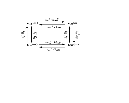
Next, defining $\kappa_{m}^{2}$ to be the non-zero eigenvalues of $-H_{AB}G_{AB}^{T}$, we thus see that the local symplectic eigenvalues can also be expressed as

$$\lambda_{m}^{2}=\frac{1}{4}+\kappa_{m}^{2}\,.$$ (41)

Now, label the mode functions corresponding to the symplectic eigenvalue $\lambda_{m}>\frac{1}{2}$ as $u_{A}^{(m)}$, $v_{A}^{(m)}$ and $u_{B}^{(m)}$, $v_{B}^{(m)}$ for sides $A$ and $B$ respectively. According to  (39) and  (21) we see that they are solutions to the eigenvalue equations

$$H_{AB}G_{AB}^{T}u_{A}^{(m)}=-\kappa_{m}^{2}u_{A}^{(m)}\,$$ (42)

$$G_{AB}H_{AB}^{T}v_{A}^{(m)}=-\kappa_{m}^{2}v_{A}^{(m)}\,.$$ (43)

and

$$H_{AB}^{T}G_{AB}u_{B}^{(m)}=-\kappa_{m}^{2}u_{B}^{(m)}\,$$ (44)

$$G_{AB}^{T}H_{AB}v_{B}^{(m)}=-\kappa_{m}^{2}v_{B}^{(m)}\,.$$ (45)

Now, multiply both sides of say  (42) on the left by $G_{AB}^{T}$, to find from  (45) that $G_{AB}^{T}H_{AB}(G_{AB}^{T}u_{A}^{(m)})=-\kappa_{m}^{2}(G_{AB}^{T}u_{A}^{(m)})$, thus showing that $v_{B}^{(m)}\propto G_{AB}^{T}u_{A}^{(m)}$. A similar procedure applied to all the above equations shows that

$$v_{B}^{(m)}\propto G_{AB}^{T}u_{A}^{(m)}\ \ \ \ v_{A}^{(m)}\propto G_{AB}u_{B}^{(m)}$$ (46)

$$u_{B}^{(m)}\propto H_{AB}^{T}v_{A}^{(m)}\ \ \ \ u_{A}^{(m)}\propto H_{AB}v_{B}^{(m)}\,.$$ (47)

The choice of the proportionality factors involved here is constrained by the normalization conditions imposed on the mode functions on both sides. A consistent choice preserving the normalization on both sides is

$$v_{B}^{(m)}=\frac{1}{\kappa_{m}}G_{AB}^{T}u_{A}^{(m)}\ \ \ \ v_{A}^{(m)}=\frac{1}{\kappa_{m}}G_{AB}u_{B}^{(m)}$$ (48)

$$u_{B}^{(m)}=-\frac{1}{\kappa_{m}}H_{AB}^{T}v_{A}^{(m)}\ \ \ \ u_{A}^{(m)}=-\frac{1}{\kappa_{m}}H_{AB}v_{B}^{(m)}\,.$$ (49)

The above relations, together with the relations  (23), yield a systematic procedure by which all the mode functions on both sides, corresponding to a given symplectic eigenvalue can be constructed once a single mode function is found. This proves particularly advantageous if the number of modes on one side is considerably smaller that in the other. This construction is summarized in figure 1.

III Harmonic Chain

A linear harmonic chain of $N$ local oscillators laid out on a circular topology may be modelled by canonical variables $(q_{i},p_{i})$ with ${i=1,..,N}$, with the dynamics given by a Hamiltonian of the form

$$H={E_{0}\over 2}\sum_{i=1}^{N}\left[p_{i}^{2}+q_{i}^{2}-\alpha\ q_{n}iq_{i+\!1}\right]\,,$$ (50)

where we identify $q_{N+1}\equiv q_{1}$ and $q_{0}=q_{N}$ and the dimensionless parameter $\alpha$ characterizing the strength of the coupling between adjacent neighbor sites is strictly less than unity. Note that such a Hamiltonian can be obtained from the standard Hamiltonian of a chain with spring-like nearest neighbor harmonic couplings

$$H=\frac{1}{2}\sum_{i=1}^{N}\left[\frac{\pi_{i}^{2}}{M}+M\omega^{2}\xi_{i}^{2}+K(\xi_{n}i-\xi_{i-1})^{2}\right]\,.$$ (51)

by means of the canonical variable re-scaling

$$q_{i}=\sqrt{M\omega\sqrt{1+\frac{2K}{M\omega^{2}}}}\,\ \xi_{i}\,,\ \ \ \ p_{i}=\frac{\pi_{i}}{\sqrt{M\omega\sqrt{1+\frac{2K}{M\omega^{2}}}}}\,$$ (52)

and the identification

$$E_{o} = {\omega\sqrt{1+\frac{2K}{M\omega^{2}}}}\,,$$ (53)

$$\alpha = \frac{\frac{2K}{M\omega^{2}}}{1+\frac{2K}{M\omega^{2}}}\,.$$ (54)

The last relation provides a restriction, $0<\alpha<1$, to the possible values of the coupling constant in  (50). The limit of strong coupling between neighboring oscillators, $\frac{2K}{M\omega^{2}}\to\infty$, corresponds to $\alpha\to 1$, and the weak coupling limit to $\alpha\to 0$.

The Hamiltonian  (50) can be brought to a normal form by introducing a set of annihilation (creation) operators $a(\theta_{k})$ ( $a^{\dagger}(\theta_{k})$ )  satisfying the commutation relations

$$[a(\theta_{k}),a^{\dagger}(\theta_{l})]=\delta_{kl}\,,$$ (55)

with the indexing angular variable $\theta_{k}$ playing the role of a dimensionless wave number or pseudo-momentum and taking the values

$$\theta_{k}=\frac{2\pi k}{N}\,,\ \ \ \ (k=0,1,\ldots,N-1)\,.$$ (56)

Defining the dispersion relation (in units of $E_{o}$)

$$\nu(\theta_{k})\equiv\sqrt{1-\alpha\cos\theta_{k}}\,,$$ (57)

and expressing $q_{n}$ and $p_{n}$ in the form

$$q_{n} = \frac{1}{\sqrt{N}}\sum_{k}\,\frac{1}{\sqrt{2\nu(\theta_{k})}}\left[a(\theta_{k})e^{i\theta_{k}n}\!+\!\mathrm{h.c.}\right]\,,$$ (58)

$$p_{n} = \frac{-i}{\sqrt{N}}\sum_{k}\sqrt{\frac{\nu(\theta_{k})}{2}}\left[a(\theta_{k})e^{i\theta_{k}n}\!-\!\mathrm{h.c.}\right]\,,$$ (59)

the Hamiltonian  (50) achieves the normal form

$$H=E_{o}\sum_{k}\nu(\theta_{k})\left[a^{\dagger}(\theta_{k})a(\theta_{k})+\frac{1}{2}\right]\,,$$ (60)

which is then diagonalized by the Fock states of the creation/annihilation operators.

In particular, we will be interested in the ground state $|0\rangle$, satisfying

$$a(\theta_{k})|0\rangle=0\,,$$ (61)

for all $\theta_{k}$. For this state, the wave functions in the coordinate and momentum representations assume the Gaussian form

$$\psi_{o}(q) \propto \exp\left[-\frac{1}{4}q^{T}G^{-1}q\right]\,,$$ (62)

$$\psi_{o}(p) \propto \exp\left[-\frac{1}{4}p^{T}H^{-1}p\right]\,,$$ (63)

where the covariance matrices $G$ and $H$, for $Q$ and $P$ respectively, satisfy the generalized uncertainty relation $GH=\frac{\openone}{4}$, with the entries defined by the two-point vacuum correlation functions:

$$G_{ij} =\langle 0|q_{i}q_{j}|0\rangle\equiv g_{(i\!-\!j)}\,,$$ (64)

$$H_{ij} =\langle 0|p_{i}p_{j}|0\rangle\equiv h_{(i\!-\!j)}\,.$$ (65)

Furthermore, since the state is Gaussian, higher moments of the oscillator coordinates or momenta are expressible in terms of the two-point correlation functions. Thus, the relevant physical information associated with the vacuum is contained in the correlation functions $g_{(i\!-\!j)}$ and $h_{(i\!-\!j)}$, which we now study.

III.1 Vacuum Correlation Functions and Three Regimes of Behavior

The general entanglement behavior of the partitioned harmonic chain is dictated by the behavior of the correlation functions $g_{l}$ and $h_{l}$ defined in Eqs.  (64) and  (65). Their explicit form is given in terms of the dispersion relation  (57) by

$$g_{l}^{(N)} \equiv \frac{1}{2N}\sum_{k}\frac{1}{\nu(\theta_{k})}\cos(l\theta_{k})\,,$$ (66)

$$h_{l}^{(N)} \equiv \frac{1}{2N}\sum_{k}\nu(\theta_{k})\cos(l\theta_{k})\,,$$ (67)

and consistent with the translational invariance of the Hamiltonian, we note their dependence only on the separation $l=(i-j)\mod N$. In the limit $N\rightarrow\infty$ with $\alpha$ fixed, these expressions yield the Riemann sum for the integral of the argument as a function of a continuous $\theta$ ranging from $0$ to $2\pi$, with the replacement of the factor of $N^{-1}$ in front by $(2\pi)^{-1}$. The correspondence with the continuum one-dimensional scalar field theory can also be obtained from these expressions by taking appropriate limits, as discussed in the appendix.

Now, for a fixed value of the strength parameter $\alpha$ and for sufficiently large values of the chain size $N$, the behavior of these functions in terms of $l$ becomes independent of $N$ and reproduces the $N\rightarrow\infty$ behavior, which can be expressed exactly in terms of hypergeometric functions as

$$g_{l}^{(\infty)} = \frac{z^{l}}{2{\mu}}\,\left(\!\begin{array}[]{c}l\!-\!\frac{1}{2}\\ l\end{array}\!\right){}_{2}\!F_{1}\left({\frac{1}{2}},l\!+\!{\frac{1}{2}},l\!+\!1,{z^{2}}\!\right)$$ (70)

$$h_{l}^{(\infty)} = \frac{{\mu}z^{l}}{2}\,\left(\!\begin{array}[]{c}l\!-\!\frac{3}{2}\\ l\end{array}\!\right){}_{2}\!F_{1}\left(-\!{\frac{1}{2}},l\!-\!{\frac{1}{2}},l\!+\!1,{z^{2}}\!\right)$$ (73)

where $\left(\begin{array}[]{c}a\\ b\end{array}\right)$ are binomial coefficients expressed in terms of Gamma functions and $z$ and $\mu$ are given by

$$z\equiv\frac{1-\sqrt{1-\alpha^{2}}}{\alpha}\,,\ \ \ \ \ \mu=\frac{1}{\sqrt{1+z^{2}}}\,.$$ (74)

This behavior in the large $N$ limit will serve as a reference in analyzing the behavior for finite $N$.

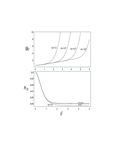
The shape of the correlations $g_{l}$ and $h_{l}$ as a function of the separation $l$ and the coupling strength is depicted in figures 2 and 3 for a fixed value of $N$. Similarly, we have plotted in 4 the behavior of their values at $l=0$ as a function of the coupling strength for different values of $N$. For these plots, we have found it convenient to introduce an ancillary hyperbolic angle $\xi$, implicitly defined by its relation to the variables $\alpha$ and $z$:

$$z=\tanh\xi\,\ \ \ \ \alpha=\tanh 2\xi$$ (75)

This becomes a convenient parameter as for small values of $\alpha$, the appropriate expansion parameter is $z$ itself, in which case $z\simeq\xi$ for $\xi\ll 1$; similarly, as $\alpha$ approaches unity, $\xi$ provides a logarithmic scale for this approach, with $\xi\simeq\frac{1}{4}\ln(1-\alpha)/2$.

Figure 2: The vacuum $g_{l}=\langle q_{o}q_{l}\rangle$ correlation function as a function of $l$ for different strength parameters where $\alpha=\tanh{2\xi}$.

Figure 3: The negative of the vacuum correlation function $h_{l}=\langle p_{o}p_{l}\rangle$ as a function of $l$ ($l\geq 1$) for different strength parameters.

Figure 4: Variances in $q$ and $p$ as a function of coupling strength for different values of $N$.

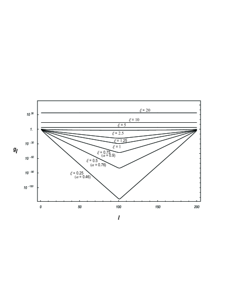
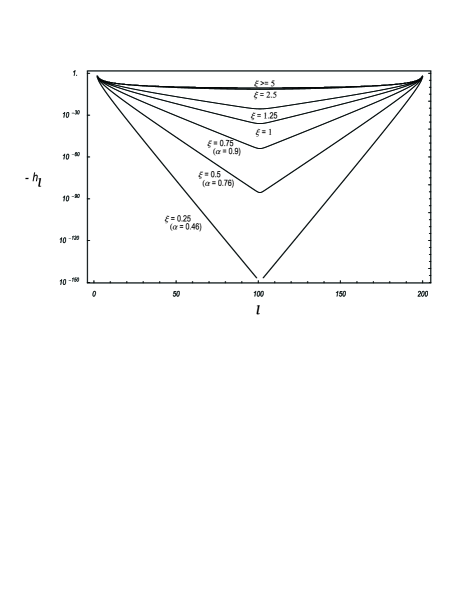
Let us first analyze the case $N=\infty$. For weak coupling, $\alpha\sim z\ll 1$, the hypergeometric functions behave as $1+o(z^{2})$; thus, with the Stirling approximation for the binomial, we obtain the weak coupling behavior

$$g_{l}\simeq\frac{1}{2\sqrt{\pi}}\,l^{-\frac{1}{2}}z^{l}\,,\ \ \ \ \ h_{l}\simeq-\frac{1}{4\sqrt{\pi}}\,l^{-\frac{3}{2}}z^{l}\,,$$ (76)

for $l\gg 1$. The weak coupling correlation functions are therefore of short-ranged, exponential behavior, and characterized by the correlation length

$$l_{c}=\frac{1}{-\ln(z)}\,.$$ (77)

On the other hand, in the limit $\alpha\simeq z\rightarrow 1$ with fixed $l$, the $g^{(\infty)}_{l}$ correlation function diverges, and is determined by the asymptotic behavior of the hypergeometric function

$${}_{2}F_{1}\left({\frac{1}{2}},l\!+\!{\frac{1}{2}},l\!+\!1,{z^{2}}\!\right)\rightarrow-\frac{\Gamma(l+1)}{\Gamma(1/2)\Gamma(l+1/2)}$$ (78)

$$\times\biggl{[}\ln\left(\frac{1-z^{2}}{4}\right)+\psi\left(l\!+\!{\frac{1}{2}}\right)+\gamma\biggr{]}(1+O(1-z))\,.$$

where $\gamma$ is the Euler-Mascheroni constant and $\psi(n)$ is the DiGamma function. With the asymptotic expansion $\psi(l+1/2)\simeq\ln l$ for large $l_{c}\gg l\gg 1$, this yields for $z\simeq 1$,

$$g_{l}\simeq-\frac{1}{\sqrt{2}\pi}\ln\left(\frac{1\!-\!z}{2}\,l\right)\,;$$ (79)

in the case of the correlation function $h_{l}$, one finds the $\alpha$ independent limit

$$\lim_{\alpha\rightarrow 1}h_{l}=-\frac{\sqrt{2}}{\pi}\frac{1}{4l^{2}-1}\,.$$ (80)

Next we consider finite-size effects. The first consideration has to do with the range the above limiting expressions given a finite size of the chain. In this respect, the exponentially decaying behavior is not expected to hold once the correlation length becomes of the order of half the chain size; similarly, the strong coupling expansion for $g_{l}$ is valid whenever the function is positive. For sufficiently large $N$, one should expect these conditions to be met at values of $\alpha$ which are close to unity, in which case $1-z\simeq\sqrt{2(1-\alpha)}$. Then the conditions $l_{c}<N/2$ and $\ln\left((1-z)N/4\right)<0$, lead essentially to the same transitional condition between short-range and long range correlation; the transition from short -ranged to long-ranged behavior then happens when a transitional correlation size scale, which we define as

$$N_{t}(\alpha)=\sqrt{\frac{2}{1-\alpha}}\,,$$ (81)

becomes of the order of $N$. Note incidentally that for $N_{t}\gg 1$, the plotting parameter $\xi$ is related to $N_{t}$ according to

$$\xi\simeq\frac{1}{2}\ln N_{t}\,.$$ (82)

The second consideration has to do with the magnitude of the correlations for $\alpha$ close to unity, which is set by the the diverging $qq$ correlation function and specifically its behavior at $l=0$. For finite but large $N$, the value of $g_{l}$ can be approximated by the $N=\infty$ expression plus corrections in powers of $N^{-1}$ arising from the error between the sum  (66) and the corresponding Riemann integral obtained when $N\rightarrow\infty$. The relevant correction comes from the contribution of the $\theta_{k}=0$ mode in  (66), which is not accounted for in the Riemann integral when the limit $\alpha\rightarrow 1$ is taken first. This contribution yields an $O(N^{-1})$ additional term, so that for $\alpha\rightarrow 1$, the finite size $g_{l}$ is approximated by

$$g_{l}^{(N)}\simeq g_{l}^{(\infty)}+\frac{1}{2N\sqrt{1-\alpha}}\,.$$ (83)

Since the correction arises from the contribution to the sum from the $\theta_{k}=0$ eigenmode, it accounts for a strong collective effect due the finite size of the chain. This correction dominates the coupling strength behavior of the $g_{l}$ correlation functions above a critical value of $\alpha$, or, for fixed $\alpha$, below a critical value of $N$. This critical value is determined by requiring that the correction term should become of the magnitude of the logarithmic term depending on the coupling strength in the strong coupling $N=\infty$ correlation function, i.e. ,

$$\frac{1}{2N\sqrt{1-\alpha}}=-\frac{1}{\sqrt{2}\pi}\ln\left(\frac{1-z(\alpha)}{2}\right)$$ (84)

Taking $\alpha$ close to unity yields finally a critical chain size value $N_{c}$

$$N_{c}(\alpha)\sim\frac{N_{t}(\alpha)}{\ln N_{t}(\alpha)}\,.$$ (85)

The above considerations allow us to distinguish three regimes of behavior for a chain size of a large and fixed value of $N$, for convenience to be referred to as the type $I$, $II$ or $III$ regimes: the type $I$, weak coupling regime, is determined by the condition $N\gg N_{t}(\alpha)>N_{c}(\alpha)$, and is characterized by short-ranged correlations; when the condition $N_{t}(\alpha)\sim N$ is met, we enter the intermediate, type $II$ long-range regime, in which the scale of correlations is of order and $\ln N_{t}(\alpha)$ and the correlations decay logarithmically as a function of $l$; finally, the condition $N_{c}(\alpha)>N$ determines the long-range, type $III$ regime, with the same logarithmic decay as a function of the distance but in which the scale of the correlations behaves as $N_{t}(\alpha)/N$. The distinction between these three regimes will serve a guideline for the characterization of the different regimes of entanglement as well.

IV An Illustrative Exactly Soluble Case

Before proceeding with the numerical results in our paper, it may be useful to consider a simple example that is easy to solve and shows very general qualitative features of the dominant entanglement structure between two complementary regions of a chain. In this case we wish to understand the entanglement of one oscillator of the chain versus the rest of the chain. For such a partition, it is quite easy to obtain the degree of entanglement by looking at the local covariance matrix of the single mode, which is given by

$$M_{A}=\left(\begin{array}[]{cc}g_{0}&0\\ 0&h_{0}\\ \end{array}\right)\,.$$ (86)

The single symplectic eigenvalue of the matrix is $\lambda=\sqrt{g_{0}h_{0}}$ and thus the degree of entanglement between the oscillator and the remainder of the chain is given is given by $S(\sqrt{g_{0}h_{0}})$ where $S$ is defined by Eq.  (12).

To understand the behavior of the degree of entanglement we look at the relevant approximations for the three regimes discussed in section  (III.1). First, expanding the hypergeometric functions in  (70) and  (73) in a power series in $z$, we obtain for the symplectic eigenvalue the weak, type $I$ regime,

$$\lambda_{I}=\frac{1}{2}+\frac{z^{2}}{8}+O(z^{4})\,.$$ (87)

Next, for strong coupling, $N_{t}(\alpha)>N$, and assuming $N\gg 1$, we approximate $h_{0}$ and $g_{0}$ by their limiting behaviors for $\alpha\rightarrow 0$. For $h_{0}$ the limiting value is $\sqrt{2}/\pi$, while for $g_{0}$ we can use the asymptotic  (78) to show that

$$g_{0}(\alpha)\simeq\frac{1}{\sqrt{2}\pi}\ln\left(4N_{t}(\alpha)\right)\,,$$ (88)

where $N_{t}(\alpha)=\sqrt{2/(1-\alpha)}$ as defined previously. Thus the symplectic eigenvalue becomes

$$\lambda_{II}\simeq\frac{1}{\pi}\sqrt{\ln(4N_{t}(\alpha))}\,;$$ (89)

this accounts for the type $II$, long-range regime with a logarithmic scale of the correlations. Finally, if, we take $\alpha$ large enough so that $N_{c}(\alpha)\gg N$, then the $g_{0}$ correlation function can be approximated by the single contribution of the collective $\theta_{k}=0$ of the whole chain

$$g_{0}(\alpha)\simeq\frac{1}{2N\sqrt{1-\alpha}}=\frac{1}{2\sqrt{2}}\left(\frac{N_{t}(\alpha)}{N}\right)\,.$$ (90)

This yields the symplectic eigenvalue

$$\lambda_{III}\simeq\sqrt{\frac{N_{t}(\alpha)}{2\pi N}}\,$$ (91)

characterizing the strong long-range (type $III$) regime.

Figure 5: Entanglement of a single oscillator versus the rest of the chain as a function of coupling strength for a chain size $N=10^{4}$ (solid). The dashed lines show the approximations of Eq.  (122): weak (I), strong transitional (II), and strong (III).

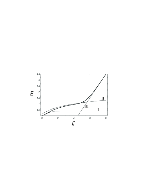
With these approximations we use the following expansions for the von-Neumann entropy  (12) as a function of $\lambda$

$$S(\lambda)\simeq\left\{\begin{array}[]{cc}(\lambda-\frac{1}{2})\left[1-\ln(\lambda-\frac{1}{2})\right]\,,&\ \ \lambda-\frac{1}{2}\ll 1\\ {}\hfil&{}\hfil\\ 1+\ln\lambda\,,&\ \ \lambda\gg 1\end{array}\right.\,.$$ (92)

This yields, for the characteristic behavior of the degree of entanglement in the three regimes, the expressions

$$E\simeq\left\{\begin{array}[]{cc}\frac{z^{2}}{8}\left[1-\ln\frac{z^{2}}{8}\right]\,,&\ \ I\ :\ N_{t}(\alpha)\ll N\\ {}\hfil&{}\hfil\\ 1+\frac{1}{2}\ln\frac{\ln 4N_{t}(\alpha)}{\pi^{2}}\ \,,&\ \ II\ :\ N_{t}(\alpha)\sim N\gtrsim N_{c}\\ {}\hfil&{}\hfil\\ 1+\frac{1}{2}\ln\frac{N_{t}(\alpha)}{2\pi N}\ \,,&\ \ II\ :\ N_{c}(\alpha)\gg N\ \ \ \,.\end{array}\right.$$ (93)

These three approximations compared quite with numerical computations of the entropy as a function of coupling strength in Fig 5 for a chain size of $N=10^{4}$. We note that the only importance dependence on the chain size for fixed coupling strength comes in the very strong regime, in which case the entanglement decreases logarithmically with $N$.

Correlated with the three regimes of behavior are the shapes of the $u$ and $v$ mode functions for the entangled mode on the complement of the chain. These are easily expressed in terms of the correlation functions $g_{l}$, $h_{l}$ using the mode-mapping diagram Fig. 1; The $l$-th components are simply given by

$$v_{l}=\frac{g_{l}}{\sqrt{g_{o}h_{o}-\frac{1}{4}}}$$ (94)

$$u_{l}=-\frac{h_{l}}{\sqrt{g_{o}h_{o}-\frac{1}{4}}} \,\ \ \ \ l=1,..,N-1\,.$$ (95)

Thus, the shapes of $u$ and $v$ are easily inferred from figures 2 and 3: in the weak regime, the mode functions exhibit rapid exponential decay away from the two sites adjacent to the singled-out oscillator; in the long-range transitional regime, the $u_{l}$ mode, being proportional to $h_{l}$, decays as the inverse squared of the distance from the edge, while the $v_{l}$ mode decays logarithmically; a similar behavior is exhibited in the strongest long-range regime, except that the $v_{l}$ mode except that the logarithmic behavior is essentially suppressed. Thus we see that in the strongest regime the entangled mode at the complement shows a collective correlated behavior in the oscillator momenta and a power-law correlation in the oscillator displacements. Two distinct limiting behaviors in $\alpha$ may then be inferred for the mode participation function of this mode, based on the asymptotics of the correlation functions, namely

$$P_{l}\sim\left\{\begin{array}[]{cc}l^{-2}z^{2l}\,,&\ \ \alpha\rightarrow 0\\ {}\hfil&{}\hfil\\ l^{-2}\,,&\ \ \alpha\rightarrow 1\end{array}\right.\,.$$ (96)

V Structure of ground state entanglement: Qualitative study and numerical results

Figure 6: Total entanglement as a function of coupling strength (in terms of $\xi$) and $N_{b}$ (log-2 scale) for a chain of size $N=2048$.

Figure 7: The three different qualitative regimes of entanglement as inferred from level curves of total entanglement in Fig. 6.

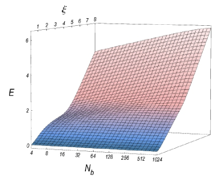
We turn then to a qualitative study of the entanglement behavior of the harmonic chain vacuum and the underlying modewise structure, based on numerical results. We shall be interested in a system of $N$ oscillators, of which the first contiguous $N_{b}\leq N/2$ constitute a subsystem that we shall refer to as the “block”, while the remaining $N-N_{b}$ will constitute what we shall refer to as the “complementary block”. From the translational symmetry of the problem, the starting point of the block on the chain is completely arbitrary.

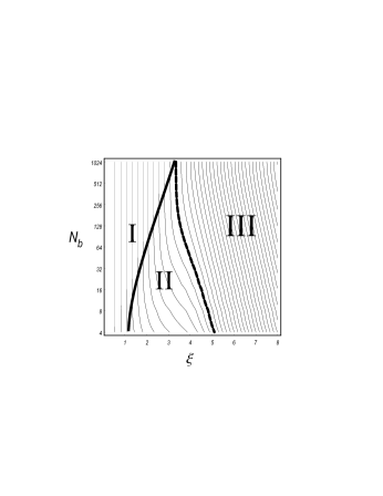
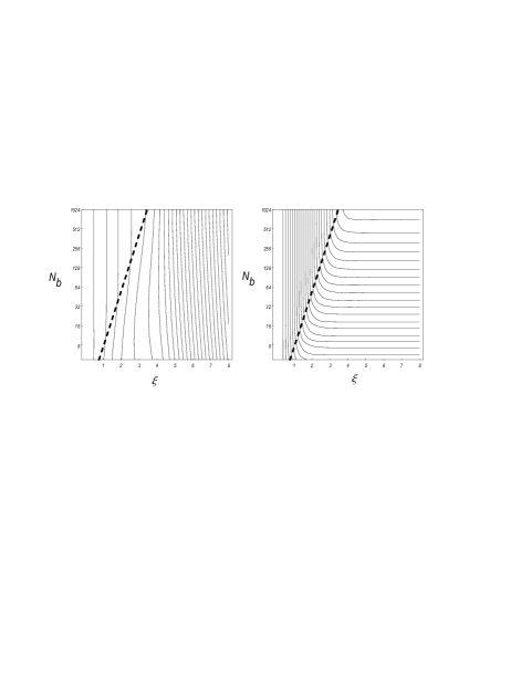
Our first survey has to do with the overall behavior of the degree of entanglement of the block and its complement as a function of the relevant properties: the size of the block $N_{b}$, the size of the chain $N$, and the coupling strength. This overall behavior has been plotted in Fig. 6, for a chain of size $N=2048$, sweeping the block size up to $N_{b}=N/2$ and the coupling strength so that $N_{c}>N$. As was seen in the previous section, the behavior of the degree of entanglement as a function of the coupling bears the signature of the three regimes outlined in section  (III.1). This signature is also evident from Fig. 6 when we look at slices of constant $N_{b}$: As a function of $\xi=\tanh(2\alpha)$, the entanglement rises from zero in the weak coupling regime to the characteristic plateau of the type $II$ regime, which is more or less centered around the value for which the transitional scale is of the order of the chain size (in our case around $\xi\simeq 3.2$); as $\xi$ is further increased, we see again the characteristic $\sim\ln N_{t}$ (i.e., linear in $\xi$) behavior of the degree of entanglement for the type $III$ regime. As we sweep then $N_{b}$ and look at the entanglement as a function of $\xi$, it then becomes possible to create an analog of a phase diagram on the $\xi-N_{b}$ plane for the qualitative behavior of the degree of entanglement; such a diagram is show in Fig. 7 and was constructed on the basis of the level curves of equal entanglement obtained to Fig. 6.

Figure 8: Entanglement as a function of $\ln N_{b}$ for $N=2048$, $\xi=12$ fitted to a straight line of slope $1/3$.

Figure 9: Entanglement as a function of block size for different values of the chain size $N$ ($\xi\simeq 3.5$).

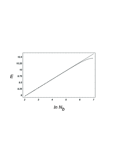
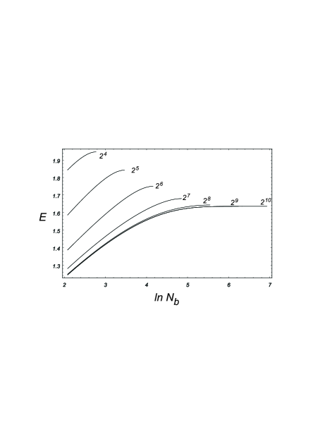
Continuing with the behavior of the total entanglement as a function of the block size, we again find distinct characteristic behaviors depending on the specific regime probed in the ”phase diagram”: for the type $I$ regime, the total degree of entanglement remains essentially constant as $N_{b}$ is varied. Clearly, this is a manifestation of the short-ranged correlations characteristic of this regime, and suggests that entanglement between the block and its complement in this regime is due essentially to edge effects. More interesting, however, is the behavior in the strong type-$II$ and type-$III$ regimes, where long range correlations are present and where therefore one should expect significant contributions from the bulk of the block. Indeed, one finds that in both of these regimes the degree of entanglement shows a logarithmic dependence on the size of the block–the one-dimensional analogue of the black hole area theorem. As shown in Fig. 8, for sufficiently large values of the coupling and $N$, and for $N_{b}\ll N$ the dependence takes the form

$$E\simeq E_{0}(\alpha,N)+\frac{1}{3}\ln N_{b}$$ (97)

reproducing the predictions of conformal field theory for the boson universality class vidalrev ; holzhey . It is also interesting to note the behavior of the value $E_{0}(\alpha,N)$ as a function of the chain size $N$ for fixed $\alpha$, which shows a similar behavior to that of the entanglement of the single oscillator mentioned in the previous section. As shown in Fig. 9, for large fixed value of $\alpha$, the $\propto\ln N_{b}$ curves decrease in height with $N$ until a critical value of $N$; below this value the $\propto\ln N_{b}$ behavior saturates at a value that is independent of the chain size.

Figure 10: Site participation function for the entangled Williamson normal modes in a chain of $N=32+48$ contiguous oscillators, at four values of the coupling strength parameter (from top to bottom): $\alpha=0.1$, $0.6$, $0.9$, $1-10^{-6}$. The mode shapes are ordered front to back according to the symplectic eigenvalue of the respective mode, with the dominant mode at the front.

Figure 11: A sample of Williamson mode shapes (solid for $u^{(m)}$, dashed for $v^{(m)}$) for a chain of size $N_{b}=74$ ($N=500$), and for weak and strong coupling. Mode ordering is according to decreasing contribution to the total entanglement.

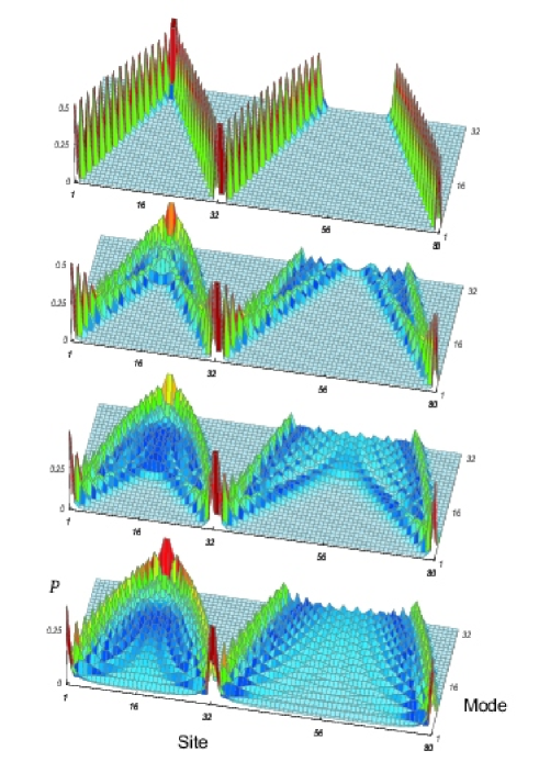
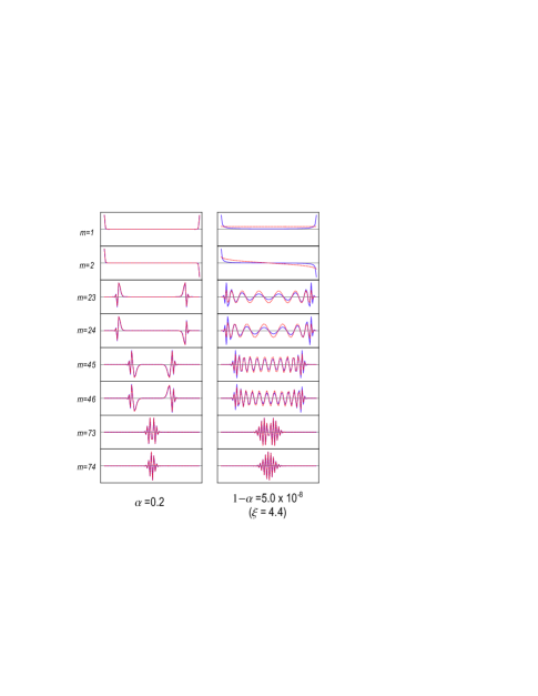
We turn then to the question of “where does the entanglement comes from ?”, from the point of view of the modewise entanglement structure of the harmonic chain vacuum. In conformity with the different regimes of behavior entailed by the correlation functions $g_{l}$ and $h_{l}$ , different behaviors are reflected in the shapes of the Williamson modes, as we illustrate in Fig. 10, which shows the site participation function for all the entangled Williamson normal modes of both the block and its complement. Figure 11 also shows a small sample of the mode shapes for the $u^{(m)}$ and $v^{(m)}$ modes, for various values of $m$, and at two different coupling strengths. A number of general features may then be identified regarding the mode structure:

The first feature, which is evident from Fig, 11, has to do with the parity of the mode functions $u^{(m)}$ and $v^{(m)}$, due to a parity selection rule to be discussed in section  (VI.1). Indexing the modes as $m=1,...N_{b}$, in increasing order of their contribution to the total entanglement, we find that in all circumstances entangled modes of either the chain or its complement have a definite parity $(-1)^{m+1}$, under reflections with respect to the center of the respective block. Thus, for each entangled mode-pair, the modes on both sides of the chain have the same parity, and the mode-pair that contributes the most amount of entanglement always involves even mode functions on both sides of the chain. This feature shows that while it may be argued that the entanglement between two regions of the chain is primarily due to edge effects, it nevertheless involves non-local behavior within each region.

Figure 12: Turning point location as a function of mode number, for three values of the coupling strength ($N_{b}=64$, $N=160$).

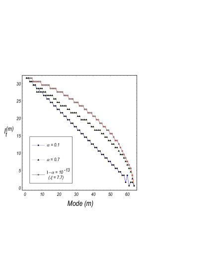
A second feature of the mode structure that is present in all circumstances is the existence of a characteristic turning point, henceforth denoted by $l_{t}^{(m)}$, which we define as the location (measured from the center of the block) of the oscillator for which the participation function $\mathcal{P}_{i}^{(m)}$ is maximal for the $m$-th mode. The general behavior of this turning point as a function of the mode number and coupling strength is shown in Fig. 12. What is observed is that $l_{t}^{(m)}$ is quite similar to the turning point of semiclassical solution to a wave equation: generally, the mode participation shows an exponential-like decay beyond the turning point, so that all the mode activity becomes effectively confined to site distances up to $l_{t}^{(m)}$ from the block midpoint; furthermore, insider this region, we find a less dramatic decay of the mode amplitudes from the turning point, achieving the minimum amplitude at the midpoint. However, in contrast to semiclassical solutions, what we find is an anti-correlation between the amplitude and the local wavelength: the longest wavelengths are present at the midpoint, whereas the oscillations become of the order of the lattice spacing at the turning point.

Figure 13: Mode shapes for the first three innermost modes for the strong regime case depicted in Fig. 13, demodulated by the oscillating factor $(-1)^{i}$. Here $n=N_{b}-m$.

The last general feature that we shall discuss is observed more prominently as the coupling strength increases, and has to do with the typical wavelength of oscillation of the mode over the majority of the interior region bounded by the turning points. This characteristic wavelength decreases with the depth ($m$) from around the order of of the chain size, for the outer mode, to the lattice spacing for the innermost modes. Interestingly, we also find a “dual” structure to the mode shape oscillations if the $u^{(m)}_{i}$ and $v^{(m)}_{i}$ mode entries are multiplied by the alternating factor $(-1)^{i}$ (corresponding to a shift of $\theta=\pi$ in their discrete Fourier transform), and the modes are ordered from the inside out. Using the index convention $n=N_{b}-m$, we find that as the coupling strength increases, the mode shapes for the lowest values of $n$ in this hierarchy of “demodulated” modes become virtually indistinguishable from harmonic oscillator wave functions of the corresponding value of $n$, with a variance of order $\sqrt{N_{b}}$ (Fig. 13). More generally, for the whole hierarchy the index $n$ labels the number of nodes in the demodulated mode functions.

Figure 14: Entanglement as a function of mode number in the weak regime, for different values of the coupling constant. Here $N_{b}=12,N=500$.

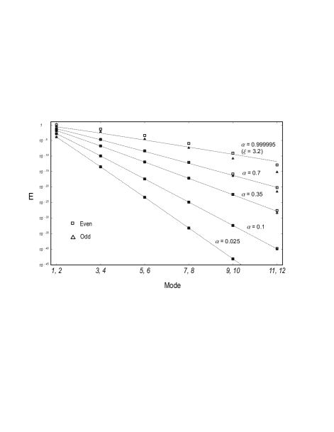
With these considerations in mind, we turn next to the characterization of the regimes of behavior discussed earlier from the standpoint of the mode structure. Beginning with the weak regime, we find that the modes for both the block and the complement fall into pairs of even and odd combinations of oscillator sites that are precisely localized in increasing distance from the edge of the block (Fig. 12), so that a mode involving a certain oscillator pair of the block is entangled with a mode of the complement involving the two oscillators’ specular images with respect to reflections about the interface. This “wedge-like” structure in the mode distribution of both sides of the chain observed in Fig. 10 can be understood in the $\alpha\rightarrow 0$ limit, where the basis of localized oscillator sites serves an eigenbasis for the whole chain; then, the leading effect of any infinitesimal coupling between contiguous oscillators is to recombine the localized modes so as to produce a mode basis consistent with the parity selection rules. We refer the reader to section VI.1 for more careful analysis discussion in this respect.

As we increase the coupling strength, and hence the correlation length $l_{c}(\alpha)$, the mode shapes become distorted to the same extent that the two participating sites lie within a distance from each other that is less than or equal to $l_{c}(\alpha)$. Thus the distortion of the modes proceeds from the inside modes of the block and then outwards as the coupling strength is increased. This distortion involves a gradual diffusion of the mode participation towards the interior region bounded by the modes, as well as the establishment of a characteristic wavelength of oscillation within this region. As the frequency spectrum of the modes becomes sharper, the width of the interior region of the mode becomes broadened, thus accounting for the gradual outward curving of the turning point location seen in Fig. 12.

Together with this mode-shape distortion, we also find the behavior of the entanglement contribution of the modes to be dictated by the correlation length in the weak regime. In Fig. 14 we have plotted on a logarithmic scale the dependence of the entanglement on the mode number in the weak regime. As stated earlier, in this regime the modes come in pairs of definite-parity combinations of oscillator sites at a precise distance from the edge; letting $d_{m}$ be this distance ($d_{m}=m/2$ for $m$ even, $(m+1)/2$ for $m$ odd) we have found that the entanglement is to leading order degenerate between modes of opposite parity and the same $d_{m}$, independent of $N_{b}$ (for $N_{b}>2$), and of exponential fall-off with $d_{m}$ according to

$$E_{m}(\alpha)\simeq\left(\frac{z(\alpha)}{4}\right)^{2(2d_{m}-1)}\left[1-2(2d_{m}-1)\ln\left(\frac{z}{4}\right)\right]\,,$$ (98)

where $z(\alpha)$ is as defined in eq. (74); from the definition  (76) of the correlation length $l_{c}$, the characteristic decay distance for the entanglement is then $l_{c}/4$. As the coupling strength is then increased, the degeneracy is lifted, with the innermost modes showing the greatest relative splitting.

This “wave” of mode distortion and degeneracy lifting continues from the inside of the chain out as the coupling increases until the correlation length becomes comparable to the size of the block and the outermost modes are distorted. As the coupling strength is increased beyond this point, no appreciable change in the shape of the modes is detected. Thus a critical value of $\alpha$ determined by

$$l_{c}(\alpha)\simeq N_{b}\,$$ (99)

sets a threshold beyond which the mode shape structure becomes frozen in its strong coupling configuration. It is this condition that underlies the transition between the type $I$ and the type $II$ transition in Fig. 7.

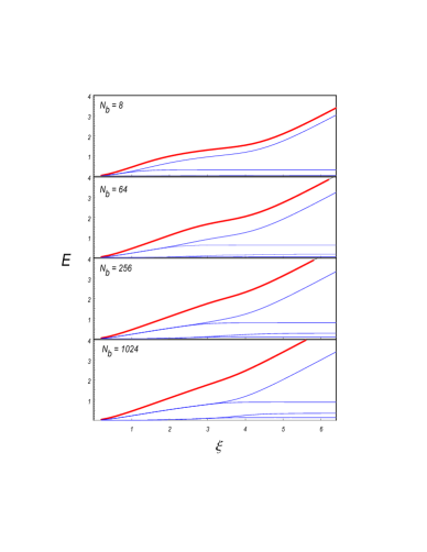
The onset of this transition and the ensuing behavior of entanglement thereafter is best appreciated from Fig. 15, where we plot, as a function of the coupling, the total entanglement and the partial entanglement from the first four dominant modes. The main signature of the transition is the lifting of the degeneracy involving the first (even) and second (odd) modes, which together up to that point are the predominant contributors to the total entanglement. Beyond that point, however, a clear decoupling occurs between the first mode and the remaining modes: the first mode accounts for the behavior of the entanglement as a function of coupling, reproducing the three-regime curve (Fig. 5) observed in section  (IV) for the case of the single entangled oscillator; on the other hand, the remaining modes become frozen in their coupling strength behavior. That this “freezing out” indeed occurs when $l_{c}(\alpha)\simeq N_{b}$ is best seen from Fig. 16, which shows the level curves on the $\xi-N_{b}$ plane for the entanglement of the first and second modes, together with a graph of the line $l_{c}(\alpha)=N_{b}$.

In this way we find that for strong coupling, the behavior of entanglement as a function of $\alpha$, particularly with respect to the type $II$ to type $III$ transition, is entirely due to the single outermost ($m=1$) Williamson mode of the block. As observed from the mode shape profiles (Fig. 11), this mode involves an essentially constant participation away from its turning points (located at the edge of the block) and may therefore be interpreted as a remnant of the $\theta_{k}=0$ collective normal eigenmode of the whole chain. In the context of the strong regimes, we shall therefore refer to this mode as the collective mode; similarly, we shall use the term residual modes for the remaining Williamson modes of the block. The reader is referred to sections  (VI.2) and  (VI.3) respectively for further analysis of the collective and residual behaviors.

Figure 15: Contribution of the first four dominant modes (thin lines) to the total entanglement (thick line) as a function of coupling strength $N_{b}$ for different values of the the block size ($N=2048$).

Figure 16: Level curves of entanglement contribution from first (left) and second (right) Williamson modes to the total entanglement depicted in Figures 6 and 7. The dotted line shows the correlation length $l_{c}$, Eq.  (76), as a function of coupling strength.

Figure 17: Contribution of the first four dominant modes (thin lines) to the total entanglement (thick line) as a function of $N_{b}$ for different values of the coupling strength ($N=2048$).

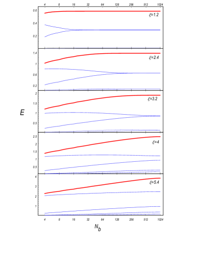
Addressing finally the large block size and chain size behavior of entanglement, we find that in contrast to the large coupling behavior, the responsible modes for the $\sim\ln N_{b}$ behavior are the residual modes. This can be seen from Fig. 17, which shows both the total entanglement and the contribution from the first four dominant modes as a function of $\ln N_{b}$ for various coupling strengths. For large enough coupling, we find that the collective mode shows a “freezing” in its $N_{b}$ behavior, while the greatest variation with $N_{b}$ is shown by the first couple residual modes. A more careful examination of the large $N_{b}$ behavior, however, indicates that the entanglement contribution of the outermost modes grows slower than $\ln N_{b}$–rather like $\ln\ln N_{b}$. Thus, the $\ln N_{b}$ behavior of the total entanglement has to be attributed to a cumulative effect from a certain number of residual modes that contribute significantly in the large $N_{b}$ limit, which turns out to be of order $\ln N_{b}$. If the modes are labelled by their characteristic frequencies, this phenomena translates to an enhancement by a factor $\ln N_{b}$ of the density of states at zero frequencypeschel04 , and corresponds in the black-hole analogy to the divergence of the density of states outside the horizon in the absence of a UV cutoffcallan .

In this respect, it is instructive to look at the entanglement contribution of all the residual modes, for which $N_{b}\ll N/2$ in the limit $\alpha\rightarrow 1$. As shown in Fig  (18), the logarithm of the entanglement of the $m$-th mode shows in this limit a scaling behavior

$$\ln E_{m}(N_{b})\sim-N_{b}f\left(\frac{m}{N_{b}}\right)$$ (100)

where $f(x)$ is some nonlinear function proportional to the central frequency of oscillation of the mode. Now, the significant contribution to the entropy comes from modes for which $\ln E_{m}$ is of magnitude unity or smaller, that is, $f\lesssim\frac{1}{N_{b}}$. As we then show in section  (VI.3), the function $f$ behaves for small values of its argument like

$$-f(x)\ln f(x)\sim x\,.$$ (101)

This behavior implies that an outer layer of residual modes, with mode numbers $m\lesssim\ln N_{b}$, yield the relevant contributions to the entropy.

Figure 18: Scaling curve of entanglement versus mode number for the strong regimes, for $N_{b}\ll N/2$. The plot includes data taken from a chain of size $N=256$ ($N_{b}$ ranging from $4$ to $32$), and chains of size $N=1024$ and $N=4096$ ($N_{b}$ ranging from $4$ to $64$), all using $\xi=10$ ($N_{c}\sim 10^{7}$).

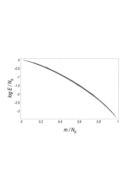
To summarize the results of our qualitative survey of the bipartite entanglement of the harmonic chain, we emphasize again the three-regime framework depicted in Fig. 7. We observe a weak coupling regime (type $I$), characterized by short range correlations, well localized modes of definite parity, and degenerate entanglement contribution from even and odd combinations of oscillator sites at the same distance from the edge. When the correlation length becomes of the order of the chain size, the mode shapes acquire a more collective behavior, a characteristic wavelength is established for each mode, and the degeneracy between contiguous modes of opposite parity is lifted. A distinction also emerges between the outermost, or “collective”, mode and the remaining (“residual”) modes. The collective mode shows a minimal contribution to the large chain size entanglement; however, it accounts for all the strong coupling constant behavior thereafter, including the transition between the type $II$ and type $III$ regimes. Conversely, the residual modes become frozen in their large coupling entanglement contribution, but are responsible for the large chain behavior. This behavior is conjectured to come from a cumulative effect from a layer of the first $\sim\ln N_{b}$ residual modes.

VI Mode structure: analytic results

We complement in this section the qualitative survey of the previous section with a more careful treatment of some of the results presented there. Our main aim is to produce simple analytic models that capture the essential elements of the modewise entanglement structure in weak and strong coupling.

VI.1 Entanglement in Weak coupling

As shown in our qualitative survey, entanglement for weak coupling involves modes that are definite parity superpositions of local oscillator-site modes. It will therefore be convenient to briefly discuss the role of parity in our problem.

Parity selection rules follow from the fact that while the local correlation matrices $(G_{A},H_{A})$ and $(G_{B},H_{B})$ lose the translational symmetry of the corresponding matrices for the whole chain, they still possess a symmetry with respect to reflections about the central indices, i.e., $G{}_{N_{b}+1-l,N_{b}+1-l}=G{}_{N_{b}+1-l,N_{b}+1-l}$. Thus, the $G$ and $H$ matrices can be written in block diagonal form as $G_{A}{}=G_{A}{}^{+}\oplus G_{A}{}^{-}$ and $H_{A}{}=H_{A}{}^{+}\oplus H_{A}{}^{-}$, in terms of blocks acting on subspaces of definite parity. Similarly, it is easy to show that with respect to the mode-mapping between the Williamson modes of the block and those of its its complement, it is also possible to show that the matrices $G_{AB}$ and $H_{AB}$ map modes of a given parity definite parity in the block to modes of the same parity in the complement. Thus, the whole problem of finding the Williamson modes in the size $N_{b}$ block, and their correlated counterparts in the complement can be reduced to two separate problems of finding Williamson modes for the sectors of size $N_{b}/2$ involving covariance matrices of definite parity.

¿From Fig. 14 it is evident that for small values of $\alpha$ the entanglement contribution decays exponentially with the mode number. This leading order exponential behavior may be understood from simple arguments based on the “wedge” shape in Fig. 10. If for a given entangled mode-pair the (properly-normalized) mode functions $u_{A}^{(m)}$, $v_{A}^{(m)}$, $u_{B}^{(m)}$ and $v_{B}^{(m)}$ are known, then the respective symplectic eigenvalue satisfies

$$\lambda_{m}^{2}=v_{A}^{(m)}{}^{T}H_{A}G_{A}u_{A}^{(m)}=\frac{1}{4}-v_{A}^{(m)}{}^{T}H_{AB}G_{BA}u_{A}^{(m)}\,.$$ (102)

Using the resolution of the identity $\openone_{B}=\sum_{\beta}v_{B}^{(\beta)}u_{B}^{(\beta)}{}^{T}$ this yields

$$\lambda_{m}^{2}=\frac{1}{4}-\sum_{\beta}v_{A}^{(m)}{}^{T}H_{AB}v_{B}^{(\beta)}u_{B}^{(\beta)}{}^{T}G_{BA}u_{A}^{(m)}\,.$$ (103)

However, we recall that $G_{BA}$ maps $u_{A}^{(m)}$ to $v_{B}^{(m)}$, meaning that the only term surviving in the sum is the one in which $\beta=m$. Thus we have that

$$\lambda_{m}^{2}=\frac{1}{4}-v_{A}^{(m)}{}^{T}H_{AB}v_{B}^{(m)}u_{B}^{(m)}{}^{T}G_{BA}u_{A}^{(m)}\,.$$ (104)

Now, in the weak coupling regime, we approximate the $m$-th even or odd mode functions in the weak regime by symmetric or antisymmetric combinations of localized site positions of depth $d_{m}$, where $d_{m}=m/2$ for $m$ even and $(m+1)/2$ for $m$ odd, as suggested by Fig. 10:

$$u_{A}^{(m\pm)}{}_{i}=v_{A}^{(m\pm)}{}_{i} = \frac{1}{\sqrt{2}}[\delta_{i,d_{m}}\pm\delta_{i,N_{b}-d_{m}+1}]$$ (105)

$$u_{B}^{(m\pm)}{}_{i}=v_{B}^{(m\pm)}{}_{i} = \frac{1}{\sqrt{2}}[\delta_{i,N_{b}+d_{m}}\pm\delta_{i,N-d_{m}+1}]\,.$$ (106)

Then, using the symmetries of the correlation functions Eq.  (104) yields

$$\lambda_{\alpha}^{2}=\frac{1}{4}-\left[h_{N_{b}}^{(N)}\pm h_{2d_{m}-1}^{(N)}\right]\left[g_{N_{b}}^{(N)}\pm g_{2d_{m}-1}^{(N)}\right]\,.$$ (107)

Next, we make use of the weak limit expressions for the correlation functions, namely that both $g_{l}$ and $h_{l}$ behave as $\sim z^{l}$, with $h_{l}$ negative for $l\geq 1$. Since $2d_{m}-1<N_{b}$ always, then the leading order expansion of $\lambda-\frac{1}{2}$ is expected to behave as $z^{2(2d_{m}-1)}$. Thus, in this approximation, the symplectic eigenvalue is seen as being due to correlations between a site in the block at a depth $d_{m}$ from the interface and a “mirror image” site in the complement at the same distance to the interface.

A careful symbolic computation of this leading order behavior for small $N_{b}$ and assuming $N=\infty$ shows that in fact the leading-order behavior of the symplectic spectrum is given by

$$\lambda_{m}(z)-\frac{1}{2}=\left(\frac{z}{4}\right)^{2(2d_{m}-1)}+o(z^{4d_{m}-1})\,.$$ (108)

This leads to a mainly exponential dependence with logarithmic corrections expressed in eq.  (98) for the entanglement per mode in the weak coupling regime, and yield the solid lines in Fig. 14, showing excellent agreement for weak coupling up to values of $z\simeq 0.7$. Our simple argument also leads us to expect from Eq.  (107) that the degeneracy between even and odd states in Eq.  (108) should be lifted by an eigenvalue splitting of order $z^{N_{b}+2m-1}$, thus becoming more significant as the mode-depth increases, and with the even parity modes having the slightly larger symplectic eigenvalue. This qualitative behavior is in fact verified in Fig. 14.

VI.2 Strong coupling–The collective mode

We turn next to the emergence of the collective mode in the strong coupling limit and its entanglement behavior. This has to do with the fact that the scale of the correlation function $g_{l}(\alpha)$ diverges as $\alpha\to 1$, together with the fact that the function behaves logarithmically as a function of $l$. Thus, the correlation function $g_{l}$ can be separated as

$$g_{l}=g_{0}(\alpha)+\Delta_{l}\,,$$ (109)

where $g_{0}$ is the diverging in $\alpha$ self-correlation function, and $\Delta_{l}$ is tends to fixed limit independent of $\alpha$. In turn, the correaltion matrix $G_{A}$ of the block takes the form

$$G_{A}\rightarrow N_{b}g_{0}\,\chi\chi^{T}+\Delta G\,,$$ (110)

where $\Delta G\sim O(1)$ and independent of $\alpha$, and

$$\chi\equiv\frac{1}{\sqrt{N_{b}}}\left(\begin{array}[]{ccccc}1&1&\ldots&1&1\\ \end{array}\right)^{T}\,.$$ (111)

Note that since for fixed $N_{b}$,

$$\lim_{g_{o}\rightarrow\infty}G_{A}\chi\rightarrow N_{b}g_{o}[\chi+o(g_{o}^{-1})]\,,$$ (112)

the vector $\chi$ becomes an eigenvector of $G_{A}$ in that limit with eigenvalue $N_{b}g_{0}$.

Similarly, since the momentum correlation functions are regular and tend to a fixed value as $\alpha\rightarrow 1$, the product $H_{A}G_{A}$ is also split into diverging and finite parts:

$$H_{A}G_{A}=N_{b}\,g_{0}(H_{A}\chi)(\chi^{T})+H_{A}\Delta G\,.$$ (113)

We now construct the vectors

$$u_{c}\propto H_{A}\chi,\,\ \ \ \ \ v_{c}\propto\chi,\,,$$ (114)

with normalization set so that $u_{c}\cdot v_{c}=1$, and define

$$g_{\chi}\equiv\chi^{T}H_{A}\chi=N_{b}g_{0}\,,\ \ \ \ \ h_{\chi}\equiv\chi^{T}H_{A}\chi\,.$$ (115)

Then, we have that

$$\lim_{g_{o}\rightarrow\infty}H_{A}G_{A}u_{c} \rightarrow g_{\chi}h_{\chi}[u_{c}+o(g_{o}^{-1})]$$ (116)

$$\lim_{g_{o}\rightarrow\infty}v_{c}^{T}H_{A}G_{A} \rightarrow g_{\chi}h_{\chi}[v_{c}^{T}+o(g_{o}^{-1})]\,,$$ (117)

showing that $u_{c}$ and $v_{c}$ become the right and left eigenvectors of $G_{A}H_{A}$ in the strong coupling limit with symplectic eigenvalue

$$\lambda^{2}_{c}=g_{\chi}h_{\chi}\,.$$ (118)

Next, we compute the value of $h_{\chi}$,

$$h_{\chi} = \chi^{T}H\chi$$ (119)

$$= \frac{1}{N_{b}}\sum_{i=1}^{N_{b}}\sum_{j=1}^{N_{b}}\left[-\frac{\sqrt{2}}{\pi}\frac{1}{4(i-j)^{2}-1}\right]$$

$$= \frac{1}{\sqrt{2}N_{b}\pi}\left[\psi\left(N_{b}+\frac{1}{2}\right)+\ln(4)+\gamma\right]\,,$$

where $\psi$ is the DiGamma function. For large $N_{b}$, we approximate

$$h_{\chi}\simeq\frac{1}{\sqrt{2}N_{b}\pi}\ln\left(4N_{b}\right)\,,$$ (120)

so that

$$\lambda_{c}^{2}\simeq\frac{g_{o}}{\sqrt{2}\pi}\ln\left(4N_{b}\right)\,$$ (121)

becomes the symplectic eigenvalue the approximation.

The behavior of the collective mode entanglement for the type-$II$ and type-$III$ regimes follows the same analysis performed in section IV for the single entangled oscillator, based on the two regimes of strong coupling behavior of $g_{o}$ determined by $N_{t}(\alpha)$ and $N_{c}(\alpha)$. Asymptotically, we find that

$$E\sim\left\{\begin{array}[]{cc}\frac{1}{2}\ln\ln N_{b}+\frac{1}{2}\ln\ln N_{t}(\alpha)\ \,,&\ N_{t}(\alpha)\sim N\gtrsim N_{c}\\ {}\hfil&{}\hfil\\ \frac{1}{2}\ln\ln N_{b}+\frac{1}{2}\ln N_{t}(\alpha)/N\ \,,&\ N_{c}(\alpha)\gg N\ \ \ \,.\end{array}\right.$$ (122)

Thus, the entanglement curve of the collective mode is essentially that of the single entangled oscillator, except for sublogarithmnc corrections dependent on the chain size $N_{b}$.

VI.3 Strong Coupling–Residual Modes

General qualitative and quantitative aspects of residual mode entanglement in the strong regime can be illustrated through a simple analytical model in the continuum, along the lines of similar models discussed in the context of geometric entropy in black hole physics callan and reduced density matrices for free electron chains peschel04 . Such models are useful in deriving the correlation between mode number, wavelength and turning point location, and thus can account for the scaling relation depicted in Fig 18, and the density of states determining the $\ln N_{b}$ behavior.

As discussed in section II, an eigenvalue problem equivalent to $HGu=\lambda^{2}u$ for a given region $A$, is the eigenvalue problem

$$Cu^{(m)}=-\kappa_{m}^{2}u_{A}^{(m)}\,,\ \ \ C\equiv H_{AB}G_{AB}^{T}\,,$$ (123)

where $H_{AB}$ and $G_{AB}$ are the matrices containing correlations between the two complementary regions $A$ and $B$, and where the eigenvalue $\kappa_{m}$ is related to the symplectic eigenvalue $\lambda_{m}$ according to $\lambda_{m}^{2}=\frac{1}{4}+\kappa_{m}^{2}\,$. We assume henceforth an infinite chain, and for the block adopt an index convention centered at the block midpoint, i.e., so that indices run from $-(N_{b}-1-1)/2$ to $(N_{b}-1-1)/2$; no loss of generality is entailed by assuming $N_{b}$ odd so that indices are integers. With these assumptions, the matrix elements of $\Gamma$ are given by the sums to infinity over both regions of the complement bordering the block

$$C_{ij}=\sum_{k=\frac{N_{b}+1}{2}}^{\infty}h_{k-i}g_{k-j}+\sum_{k=\frac{N_{b}+1}{2}}^{\infty}h_{k+i}g_{k+j}\,.$$ (124)

We base our computation of $C$ on the asymptotic expressions for the correlation functions  (78) and  (78), retaining the terms yielding the leading order behavior in $N_{b}$ upon converting the above sums to integrals. Thus we use

$$g_{i-j} \simeq g_{0}-\frac{1}{\sqrt{2}\,\pi}\ln|i-j|\,,$$

$$h_{i-j} \simeq -\frac{1}{2\sqrt{2}\,\pi}\frac{1}{|i-j|^{2}}\,.$$ (125)

where we include the diverging part $g_{0}$ corresponding to the collective mode. Replacing the sums in  (124) by integrals in $k$ from $N_{b}/2$ to infinity, and defining the scaled variables $x\equiv i/N_{b}$, and $y\equiv i/N_{b}$, we finally obtain a result of the form

$$C(i,j)=N_{b}^{-1}\Gamma(x,y)\,,\ \ \ \ \Gamma=\Gamma_{CS}+\Gamma_{CA}+\Gamma_{R}\,,\ \ \$$ (126)

where

$$\Gamma_{CS} = -\frac{\sqrt{2}}{4\pi(\frac{1}{4}-y^{2})}\left[g_{0}-\frac{\ln(N_{b}\sqrt{\frac{1}{4}-x^{2}})}{\sqrt{2}\pi}\right]$$

$$\Gamma_{CA} = \frac{x}{4\pi^{2}(\frac{1}{4}-x^{2})}\,\ln\left(\frac{1+2y}{1-2y}\right)$$

$$\Gamma_{R} = \frac{1}{4\pi^{2}(x-y)}\ln\left(\frac{(1+2x)(1-2y)}{(1-2x)(1+2y)}\right)\,.$$ (127)

The matrices $\Gamma_{CS}$ and $\Gamma_{CA}$ are of rank one and determine the behavior of the dominant mode for the even and odd sectors respectively; in turn, the bulk of the residual modes is determined by $\Gamma_{R}$.

To probe the solutions to the above eigenvalue problem, we next consider the continuum generalization,

$$\int_{-1/2}^{1/2}dy\,\Gamma(x,y)\,\psi(y)=-\kappa^{2}\psi(x)\,.$$ (128)

For this, it will be convenient to perform a change of variables suggested by  (VI.3), mapping the interval $(-1/2,1/2)$ to the real line

$$u=\ln\left(\frac{1+2x}{1-2x}\right)\,,\ \ \ v=\ln\left(\frac{1+2y}{1-2y}\right)\,,$$ (129)

and rescale the wave function according to

$$\tilde{\psi}(u)=\frac{1}{4}\cosh^{-2}\left(\frac{u}{2}\right)\,\psi(u)\,.$$ (130)

The new eigenvalue equation then reads

$$\int_{-\infty}^{\infty}dv\,\tilde{\Gamma}(u,v)\,\psi(v)=-\kappa^{2}\psi(u)\,,$$ (131)

where the new kernel $\tilde{\Gamma}(u,v)$ is split in the form $\tilde{\Gamma}_{CS}+\tilde{\Gamma}_{CA}+\tilde{\Gamma}_{R}$, with the respective terms given by

$$\tilde{\Gamma}_{CS} = -\frac{\sqrt{2}}{4\pi}g_{0}-\frac{1}{4\pi^{2}}\left[\ln\left(\frac{N_{b}}{2\cosh\left(\frac{v}{2}\right)}\right)-\frac{u}{2}\tanh\left(\frac{u}{2}\right)\right]$$

$$\tilde{\Gamma}_{CA} = \frac{v}{4\pi^{2}}\tanh\left(\frac{u}{2}\right)$$

$$\tilde{\Gamma}_{R} = \frac{1}{8\pi^{2}}\,\frac{u-v}{\tanh\left(\frac{u-v}{2}\right)}\,.$$ (132)

We now use $\tilde{\Gamma}\simeq\tilde{\Gamma}_{R}$ for the inner modes, which amounts to neglecting the lowest wavelength solutions. In this case, it is straightforward to see that the plane wave function $\tilde{\psi}(u)=\exp(i\omega u)$ is an eigenfunction of $\tilde{\Gamma}_{R}$. The resulting integral for the eigenvalues can be performed by contour methods and yields

$$\kappa_{R}^{2}=-\frac{1}{8\pi^{2}}\int_{-\infty}^{\infty}dv\frac{v\,e^{i\omega v}}{\tanh\left(\frac{v}{2}\right)}\,=\frac{1}{4}\sinh^{-2}(\pi\omega)\,.$$ (133)

Finally, reverting to the variables $x$, $y$ and taking even/ odd combinations of the plane wave solutions, we find as finite- wavelength eigenfunctions of the continuum eigenvalue problem  (128), the solutions

$$\psi(x)=\frac{1}{1-4x^{2}}\left\{\begin{array}[]{c}\cos(S_{\omega}(x))\\ \sin(S_{\omega}(x))\end{array}\right\}$$ (134)

where

$$S_{\omega}(x)=\omega\ln\left(\frac{1+2x}{1-2x}\right)\,,$$ (135)

The local wavenumber of these solutions, $S^{\prime}_{\omega}(x)$, increases from the value $4\omega$ as one moves away from the midpoint and diverges at the boundaries ($x=\pm 1/2$). Similar mode functions were obtained in peschel04 for the eigenmodes of the reduced density matrix of the free-electron chain. Note that the symplectic eigenvalues are

$$\lambda=\sqrt{\frac{1}{4}+\frac{1}{4}\sinh^{-2}(\pi\omega)}=\frac{1}{2}\coth(\pi\omega)\,,$$ (136)

so the Boltzmann-like $\beta_{m}$ factors associated with each Williamson mode according to eqs.  (11) are given by $\beta=2\pi\omega$. For large $\beta$, this yields an asymptotic expansion of the entropy $E\sim e^{-2\pi\omega}$, from which the scaling relation depicted in Fig. 18 should then be expected to follow.

We next connect these solutions to the corresponding solutions of the discrete chain. The first thing to note is that in the continuum approximation, the discrete modes correspond to averages of the continuum modes over the lattice spacing. Thus, the diverging oscillatory behavior of the continuum modes as the block edge is approached holds only up to a certain distance from the edge in the discrete approximation, corresponding to the point where the local oscillation wavenumber becomes of the order of the cutoff imposed by the lattice spacing. As one moves towards the edges beyond this point, the oscillations are washed out in the average and thus the mode amplitude decays. This is consistent with the fact, noted in section V, that at the turning points each Williamson mode shows oscillations of the maximum wavenumber. The turning points are therefore fixed by the condition that

$$\zeta\left|\frac{dS}{dx}\right|_{x=\pm x_{t}}=\pi N_{b}$$ (137)

where $\zeta$ is number of order unity. With the definition $~{}(\ref{defs})$, this yields the relation between the turning point and $\omega$

$$x_{t}=\frac{1}{2}\sqrt{1-\zeta\frac{4\omega}{\pi N_{b}}}\,.$$ (138)

Once the turning point is identified as a function of $\omega$, we can work out the quantization of the modes. For this we use the fact observed from our numerical calculations in section V, that when the interior modes are modulated by the oscillating factor $(-1)^{i}$–corresponding to frequency shift by the cutoff frequency–the modes show a hierarchy in which each mode can be labelled by the number of nodes $n+N_{b}-m$. Writing the modulated functions like

$$\psi_{\mathrm{mod}}(x)=(-1)^{i}\psi(x)=\frac{1}{1-4x^{2}}\cos(\pi N_{b}x-S_{\omega}(x))\,,$$ (139)

and similarly for the antisymmetric mode, we demand that $\psi_{\mathrm{mod}}(x)$ show $n$ nodes between the turning points; in this way we obtain the quantization condition

$$\pi N_{b}x_{t}(\omega)-S_{\omega}(x_{t}(\omega))=\frac{n\pi}{2}\,.$$ (140)

The resulting equation for $\omega$ is best cast in a form that can easily be interpreted from the scaling relation of the entropy  (100). For this we define the dimensionless parameters

$$f\equiv\frac{4\omega}{\pi N_{b}}\,\ \ \ \ \mu=\frac{m}{N_{b}}\,,$$ (141)

where $m=N_{b}-n$ labels the modes from the outside in, and $f$ measures the central wavelength of the mode relative to the cutoff wavelength $\pi N_{b}$; for large $\omega$, the entanglement of the mode is therefore given by

$$N_{b}^{-1}\ln E=\frac{\pi^{2}}{2}f(\mu)\,,$$ (142)

in accordance with equation  (100). From the quantization condition  (140), the function $f(\mu)$ is then the solution to the equation

$$1-\sqrt{1-\zeta f}+\frac{f}{2}\ln\left(\frac{1+\sqrt{1-\zeta f}}{1-\sqrt{1-\zeta f}}\right)=\mu\,.$$ (143)

For the outermost modes, corresponding to small $\mu$, small $f$, the relation becomes independent of $\zeta$ to leading order and reduces to

$$f\ln f=-2\mu\,,$$ (144)

as mentioned earlier. On the other hand, the fit for the innermost modes is sensitive to the precise value of $\zeta$. We have found that a value of $\zeta\simeq 0.45$ yields a remarkably good fit to the numerical data (Fig 19), as well as the turning point location depicted in Fig. 12.

It is worth mentioning that in the present approach, the role of a cutoff frequency for the continuum is not only reflected in a cutoff of the resulting frequency spectrum of the reduced density matrix, but also entails a localization of the mode functions away from the interface between the block and the complement. The condition determining the turning point can only be approximately estimated from the continuum model and therefore fails to account for the exponential fall-off of the amplitude beyond the turning point. The method also fails to account for the $\Delta x\sim N_{b}^{-1/2}$ scaled width of the the innermost mode functions , which is sensitive to the fall-off details.

Figure 19: Comparison between analytical and numerical results for the scaled central wavelength $f$ as a function of the scaled mode number, using $\zeta=0.45$.

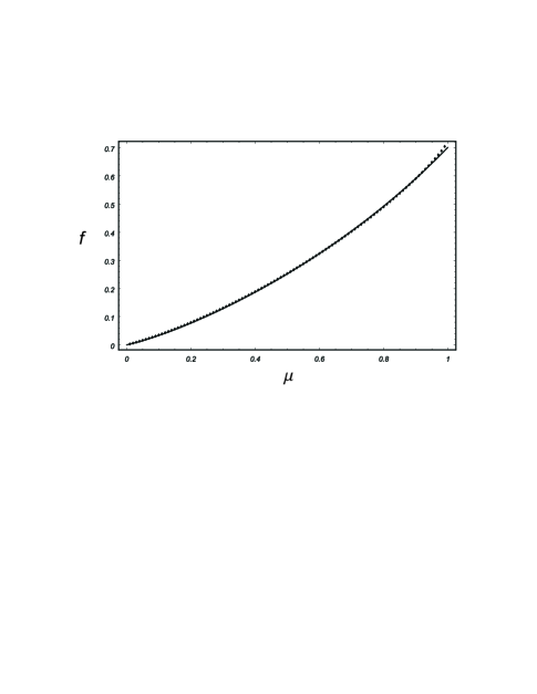
VI.4 Residual mode contribution to the Entropy

To obtain the asymptotic $\ln N_{b}$ behavior for $N_{b}\ll N$, we note that the significant contributions to the entropy will come from modes for which $\omega$ is of order unity or smaller, since the entanglement is suppressed exponentially for $\omega>1$; since this implies that $f$ will be of order $1/N_{b}$ or smaller, the approximation  (144) becomes more accurate for these modes as $N_{b}\rightarrow\infty$. Thus, discarding terms of order unity in the logarithm, the eigenvalue equation for $\omega$ can be cast in the implicit form

$$\omega_{m}=\frac{m\pi}{2\ln(N_{b})\left[1-\frac{\ln\omega}{\ln N_{b}}\right]}\,.$$ (145)

Next, we can argue that as $N_{b}\rightarrow\infty$, the term in brackets in the denominator of  (145)can be neglected for the calculation of the entanglement; this term becomes important when $N_{b}^{-1}\sim\omega\ll 1$ in the lower (since $\omega\gtrsim 1$, the approximation is already warranted in the upper end). For the lower end, we consider the smallest posible value of $\omega$, for $m=2$; according to  (145), this value is of order of $1/\ln N_{b}$ and is therefore of an order $N_{b}/\ln N_{b}$ greater than the scale at which  (145) deviates from linearity. Hence we find the approximate linear expression for $\omega$,

$$\omega_{m}\simeq\frac{m\pi}{2\ln(N_{b})}\,,$$ (146)

for the range of modes yielding relevant contributions to the entanglement as $N_{b}\rightarrow\infty$. Using the approximation $E(\beta)\simeq 1-\ln\beta$ for $\beta\ll 1$, the entanglement of the modes for which $\ln N_{b}\gg m\geq 2$, can then be estimated to be

$$E_{m}\simeq-\ln\left(\frac{\pi^{2}m}{\ln N_{b}}\right)\,.$$ (147)

Consequently, the outermost residual modes yield a contribution of order $\ln\ln N_{b}$, in the same way that the collective mode behaves for large $N_{b}$.

To obtain the leading term in the asymptotic expansion of the the total residual mode entanglement, we note that for $N_{b}\gg m\gg\ln N_{b}$ the entanglement contribution is suppressed, the total residual entanglement can be estimated to be

$$E_{R}\simeq\left.\left(\frac{dm}{d\beta}\right)\right|_{0}\int_{0}^{\infty}d\beta\,S(\beta)$$ (148)

where

$$S(\beta)=\frac{\beta}{e^{\beta}-1}-\ln(1-e^{-\beta})\,,$$ (149)

and where we evaluate the density of states assuming a linear relation at $\beta=\omega=0$ (note that this approximation entails neglecting terms of order $o(\ln\ln N_{b})$ and lower). With an integration by parts, the entropy can expressed as

$$E_{R}=2\left(\frac{dm}{d\beta}\right)\int_{0}^{\infty}\,d\beta\,\frac{\beta}{e^{\beta}-1}+O(\ln\ln N_{b})\,,$$ (150)

and from  (146), the density of states is given by

$$\frac{dm}{d\beta}=\frac{1}{2\pi}\frac{dm}{d\omega}=\frac{1}{\pi^{2}}\ln N_{b}\,.$$ (151)

The integral is standard in statistical mechanics and is given by $\pi^{2}/6$. Thus we find that as $N_{b}\rightarrow\infty$, the residual mode entropy is given by

$$E_{R}=\frac{1}{3}\ln N_{b}\,+O(\ln\ln N_{b})\,,$$ (152)

as expected.

VII Comparison with previous results

In this section we comment on the relation of our results with earlier work. Audenaert et. al. plenio have studied the entanglement in the circular linear chain model, for various choices of bipartite divisions. In this work, the logarithmic negativity log-negativity has been used as a measure for entanglement. Interestingly, we find that the von-Neumann entanglement seems to be, in the present problem, a more sensitive quantifier of the connection between entanglement and correlations. In Section IIIa we showed that the behavior of vacuum correlation functions quantifies three regimes: a weak coupling regime characterized by short-ranged correlations, an intermediate regime that is reached when the correlation length is of the order of the whole chain, and finally, a long range correlation regime. The transition between these regimes is clearly manifested in the behavior of the von-Neumann entropy (see Figs. 5, 7, 15), but is absent in the behavior of the logarithmic negativity. The difference also shows up when comparing the dependence of the two measures on the total chain size $N$. In the particular case where $N_{b}=N/2$ (plenio , corollary 1), the logarithmic negativity shows no $N$ dependence. The von-Neumann entropy, on the other hand, decreases as a function of $N$ like $\ln(N_{t}/N)$ (see eqs. (4.8), (6.21) and Fig. 9). This dependence on $N$, can be physically understood as due to the contribution of the collective mode to the entanglement, which reduces with increasing $N$. Thus is seems that the logarithmic negativity is not sensitive to the contribution of the collective mode.

The entanglement of a finite region for a one dimensional field bosonic and fermionic fields has been previously investigated in connection with the black hole entropy “area law” bombelli ; srednicki ; dowker . By employing methods of conformal field theory it has been shown callan ; holzhey ; kabat that in the massless case entanglement behaves like

$${c+\bar{c}\over 6}\ln{L\over\epsilon}$$ (153)

where $\epsilon$ plays the role of the UV cutoff, and $c$ and $\bar{c}$ are the holomorphic and anti-holomorphic central charges of the conformal field theory, with $c=\bar{c}=1$ for bosons, and $c=\bar{c}=1/2$ for fermions. Thus the overall coefficient is given by either 1/3 for bosons, or 1/6 for fermions. The same type of universal behavior has been recently derived the XY and Heisenberg spin-chain models vidal .

In the present work, we obtained a logarithmic dependance of the entanglement $\frac{1}{3}\ln N$, corresponding as expected to a bosonic field (Fig.  (8)). Furthermore we have seen that the logarithmic increase of the can be understood as an increase in the number of relevant contributing modes while the coefficient $1/3$ can be obtained from the density of the modes. As in previous results, these modes can be identified to be in a layer that becomes infinitesimally narrow in the limit of large $N$. However, no attention has so far been given to the structure of the inner modes. A central outcome of the present work is that the inclusion of an ultraviolet cutoff, which is needed for the consistency of the one dimensional field theory, gives rise to a localization of the highest frequency modes around the midpoint of the region. Although the contribution of these modes to the entanglement is exponentially small it is plausible that these inner modes play an important role in the persistence of vacuum entanglement between separated regions as we suggest in the next section.

A number of results presented in this paper can also be related to previously obtained results for both fermions and bosons in the context of the density matrix renormalization group (DMRG)whiteDMRG ; whiterev ; peschel04 ; peschel98 ; peschel99 ; peschel00 . In particular, the factorized thermal form of the reduced density matrices, the shape of the corresponding mode functions in the continuum limit, and the approximately linear behavior of the frequency spectrum for the outermost modes have been studied extensively in that context. It is possible that the method used in Section VI.3, whereby the cutoff imposed by the lattice spacing is used to establish the turning points and quantization condition of the mode functions, may prove useful for the DMRG scheme.

VIII Summary and discussion

Previous work on ground state entanglement in chain-like systems has mostly focused on the dependence of the amount of entanglement on parameters such as the block size, the separation between sites and the nature of the bipartite splitting. While in the present work we have reproduced several earlier results, as discussed in the previous section, the emphasis here has been on the study of the spatial entanglement structure emerging from the modewise decomposition of the ground state wave function.

From this analysis, we have identified certain general properties of the mode structure and its relation to the entanglement contribution. A first feature is localization–a definite characteristic distance from the division interface for the entangled modes at either side of the interface, thus establishing a characteristic distance separating the entangled mode functions. This in turn, serves to characterize the strength of the entanglement, which decays exponentially with this distance.

A second feature, which becomes sharper with increasing coupling strength, is a characteristic wavelength correlated with the degree of localization of the modes. This correlation is in fact observed in two guises: on the one hand, it provides an alternative characterization of the modes in terms of their central wavelength, with the innermost modes possessing the shortest wavelength dictated by the lattice spacing; on the other hand, the amplitude of each mode is correlated to the local oscillation wavelength, with the largest amplitude occurring when a the cutoff wavelength.

We have shown that the effect of the interaction strength on the shape of the modes and their contribution to entanglement is fundamentally connected with the correlation length. When the coupling is strong enough such as the correlation length becomes comparable to the size of the system, and the system becomes effectively massless, scale free behavior emerges for the bulk of the modes. The shape of the mode functions can be connected to the scale free continuum field theory, and both the localization and the characteristic wavelength scale with the size of the block.

On a more speculative note, it is possible the results of this paper may shed new light into several features of mixed state entanglement for separated non-complementary regions in vacuum. It has been shown that for arbitrarily separated regions, vacuum entanglement persists and Bell inequalities are violated vac-bell-ineq , with a lower bound of the entanglement that goes like $\exp(-L^{2}/D^{2})$ where $D$ and $L$ denote the size of the regions and their separation. It was shown that a large probe energy gap is required in order to extract this entanglement. This seems to suggest that the localization of the inner modes and their short wavelength characteristic are linked with the persistence of vacuum entanglement at large distances. It is possible this persistence represents an effective shielding of the entanglement content of the innermost modes. This qualitative argument could help explain the truncation effect that takes place beyond a critical distance in the discrete version of this problem when the region sizes are kept fixed, and could explain the discrepancy between entanglement and correlation lengths in other models.

IX Appendix: Discretization of the Massive Continuum Theory

In this appendix we connect our results for the discrete chain with a continuum bosonic theory in one dimension. To this end, consider the Hamiltonian for the one-dimensional massive continuum theory on a circular topology

$$H=\frac{1}{2}\int dx\,\left[\pi(x)^{2}+(\phi^{\prime}(x))^{2}+\mu^{2}\phi(x)^{2}\right]\,,$$ (154)

where we assume that $x$ runs from $-L/2$ to $L$ and that $\phi(x-L/2)=\phi(x+L/2)$, and field configuration and momentum operators satisfying the commutation relations

$$[\phi(x,t),\pi(y,t)]=i\delta(x-y)\,.$$ (155)

The Hamiltonian is diagonalized in terms of normal mode creation (annihilation) operators $a(k_{n})(a(k_{n})^{\dagger})$ with $k_{n}=\frac{2\pi}{L}n$, $n\in\mathbb{Z}$, and such that $[a(k_{n}),a(k_{m})^{\dagger}]=\delta_{n,m}$. The fields are then given by

$$\phi(x) = \frac{1}{\sqrt{L}}\sum_{n}\,\frac{1}{\sqrt{2\omega(k_{n})}}\left[a(k_{n})e^{ik_{n}x}\!+\!\mathrm{h.c.}\right]\,,$$ (156)

$$\pi(x) = \frac{-i}{\sqrt{L}}\sum_{n}\sqrt{\frac{\omega(k_{n})}{2}}\left[a(k_{n})e^{ik_{n}x}\!-\!\mathrm{h.c.}\right]\,,$$ (157)

where $\omega(k)$ is the usual dispersion relation $\omega(k)=\sqrt{\mu^{2}+k^{2}}$. The continuum field correlation functions can then be obtained yielding

$$\tilde{g}^{(L)}(x) = \frac{1}{2L}\sum_{n}\frac{\cos(k_{n}x)}{\omega(k_{n})}\,$$ (158)

$$\tilde{h}^{(L)}(x) = \frac{1}{2L}\sum_{n}\omega(k_{n})\cos(k_{n}x)$$ (159)

In the limit when $L\rightarrow\infty$, these expressions can be expressed in terms of the modified Bessel functions:

$$\tilde{g}^{(\infty)}(x) = \frac{1}{4\pi}\int_{-\infty}^{\infty}dk\frac{\cos(kx)}{\sqrt{k^{2}+\mu^{2}}}$$ (160)

$$= \frac{1}{2\pi}K_{0}(\mu|x|)$$ (161)

$$\tilde{h}^{(\infty)}(x) = \frac{1}{4\pi}\int_{-\infty}^{\infty}dk\sqrt{k^{2}+\mu^{2}}\ \cos(kx)$$ (162)

$$= -\frac{\mu}{2\pi x}K_{1}(\mu|x|)$$ (163)

The asymptotic form of the correlation functions is given for $x\ll\mu^{-1}$ by

$$\tilde{g}^{(\infty)}(x) \rightarrow -\frac{1}{2\pi}\left[\ln\left(\frac{\mu|x|}{2}\right)+\gamma\right]$$ (164)

$$\tilde{h}^{(\infty)}(x) \rightarrow -\frac{1}{2\pi|x|^{2}}$$ (165)

and for $x\gg\mu^{-1}$, we have

$$\tilde{g}^{(\infty)}(x) \rightarrow -\frac{e^{-\mu|x|}}{2\sqrt{2\pi\mu|x|}}$$ (166)

$$\tilde{h}^{(\infty)}(x) \rightarrow \sqrt{\frac{\mu}{8\pi|x|^{3}}}e^{-\mu|x|}$$ (167)

The theory at the continuum may be approximated by a linear chain of $N$ sites in a ring topology, introducing discretized variables $q_{n}$ and $p_{n}$, which up to scale changes samples the field and its conjugate momentum field at points $x_{n}=-L/2+\frac{n}{N}L$. To obtain a Hamiltonian of the form  (50), we first approximate the field Hamiltonian by replacing $\int dx\rightarrow\frac{L}{N}\sum_{n}$, $\phi^{\prime}(x_{n})\rightarrow\frac{N}{L}(\phi_{n}\!-\!\phi_{n-1})$. Then we perform the following transformation

$$\phi(x_{n})=\sqrt{\frac{N}{L}}\,\Lambda^{-1/2}\,q_{n}\,,\ \ \ \pi(x_{n})=\sqrt{\frac{N}{L}}\,\Lambda^{1/2}\,p_{n}$$ (168)

It is can now be seen that with the choice

$$\Lambda=\left[2\left(\frac{N}{L}\right)^{2}+\mu^{2}\right]^{1/2}\,.$$ (169)

we obtain a Hamiltonian of the form  (50) with

$$E_{o}=\Lambda$$ (170)

and an effective coupling strength

$$\alpha(\mu L/N)=\frac{1}{1+\frac{1}{2}\left(\frac{\mu L}{N}\right)^{2}}=1-\left(\frac{\mu}{\Lambda}\right)^{2}\,.$$ (171)

The correlation functions in the continuum are characterized by the length scale $1/\mu$. As can be seen from eqs. (164-167),for separation $x<1/\mu$ the theory behaves essentially as massless, while for $x>1/\mu$, the correlations decay exponentially. This length scale can then be related to the correlation length obtained from the infinite harmonic chain by the relation $\mu a\leftrightarrow N_{c}(\alpha)=\sqrt{2\over{1-\alpha}}$. We can then verify that the following relations hold between the discrete and continuum correlation functions

$$\tilde{g}^{L}(x) = \frac{1}{\sqrt{2}}\lim_{N\rightarrow\infty}\left.g^{(N)}_{n(x,N)}\right|_{\alpha(\mu L/N)}$$ (172)

$$\tilde{h}^{L}(x) = \sqrt{2}\lim_{N\rightarrow\infty}\left(\frac{N}{L}\right)^{2}\left.h^{(N)}_{n(x,N)}\right|_{\alpha(\mu L/N)}$$ (173)

In finite massive chains, another useful limits are

$$\tilde{g}^{\infty}(x) = \frac{1}{\sqrt{2}}\lim_{\Lambda\rightarrow\infty}\left.g^{(\infty)}_{n=x\Lambda/\sqrt{2}}\right|_{\alpha(\mu/\Lambda)}$$ (174)

$$\tilde{h}^{\infty}(x) = {\sqrt{2}}\lim_{\Lambda\rightarrow\infty}\Lambda^{2}\left.h^{(\infty)}_{n=x\Lambda/\sqrt{2}}\right|_{\alpha(\mu/\Lambda)}$$ (175)

or equivalently

$$\tilde{g}^{\infty}(x) = \frac{1}{\sqrt{2}}\lim_{l\rightarrow\infty}\left.g^{(\infty)}_{l}\right|_{\alpha=1-\frac{1}{2}\left(\frac{\mu x}{l}\right)^{2}}$$ (176)

$$\tilde{h}^{\infty}(x) = \sqrt{2}\lim_{l\rightarrow\infty}\left(\frac{x}{l}\right)^{2}\left.h^{(\infty)}_{l}\right|_{\alpha=1-\frac{1}{2}\left(\frac{\mu x}{l}\right)^{2}}$$ (177)

References

- (1) T. J. Osborne and M. A. Nielsen, Phys. Rev. A 66, 032110 (2002). quant-ph/0202162.
- (2) A. Osterloh, L. Amico, G. Falci, R. Fazio, Nature 416, 608 (2002). quant-ph/0202029.
- (3) G. Vidal, J. I. Lattore, E. Rico and A. Kitaev, Phys. Rev. Lett. 90 227902 (2003). quant-ph/0009041
- (4) J. I. Latorre, E. Rico, G. Vidal, quant-ph/0304098.
- (5) B. Q. Jin, V. E. Korepin, quant-ph/0304108.
- (6) P. Zanardi, X. Wang J. Phys. A, 35 7947 (2002). quant-ph/0201028.
- (7) M.A. Martín-Delgado, quant-ph/0207026.
- (8) K. Audenaert, J. Eisert M. B. Plenio and R. F. Werner, Phys. Rev. A 66, 042327 (2002). quant-ph/0205025.
- (9) M. B. Plenio, J. Hartley and J. Eisert, New. J. Phys. 6 36 (2004). quant-ph/0402004.
- (10) V. Vedral, quant-ph/0302040.
- (11) C. Callan and F. Wilczek, Phys.Lett.55 B333 (1994). hep-th/9401072.
- (12) D. Kabat and M. J. Strassler ,Phys.Lett. B329, 46 (1994). hep-th/9401125.
- (13) C. Holzhey, F. Larsen, F. Wilczek, Nucl.Phys. B424 (1994) 443 (1994). hep-th/9403108.
- (14) L. Bombelli, R. Koul, J. Lee and R. Sorkin, Phys. Rev. D 71, 66 (1986).
- (15) M. Srednicki, Phys. Rev. Lett. 71, 666 (1993). hep-th/9303048.
- (16) J. S. Dowker, Class.Quant.Grav. 11, L55 (1994). hep-th/9401159.
- (17) F. Verstraete, M. Popp, J.I. Cirac Phys. Rev. Lett. 92, 027901 (2004). quant-ph/0307009.
- (18) F. Verstraete, M.A. Martin-Delgado, J.I. Cirac, Phys. Rev. Lett. 92, 087201 (2004). quant-ph/0311087.
- (19) J. K. Pachos, M. B. Plenio, quant-ph/0401106
- (20) A. Botero and B. Reznik, unpublished.
- (21) J. Eisert, M.B. Plenio, Quant. Inf. Comp. 1, 479 (2003).
- (22) A. Botero and B. Reznik, Phys. Rev. A 67, 052311(2003). quant-ph/0209026.
- (23) G. Giedke, J. Eisert, J.I. Cirac, M.B. Plenio, Quant. Inf. Comp. 3, 211 (2003), quant-ph/0301038.
- (24) B. Reznik, Found.Phys.33:167-176,2003. quant-ph/0008006, quant-ph/0212044.
- (25) B. Reznik, A. Retzker, J. Silman, quant-ph/0310058.
- (26) J. Williamson, Amer. J. Math. 58, 141 (1936).
- (27) R. Simon, E.C.G. Sudarshan and N. Mukunda, Phys. Rev. A 36 3868 (1987).
- (28) R. Simon, N. Mukunda and B. Dutta, Phys. Rev. A 49, 1567 (1994).
- (29) I. Peschel, cond-mat/0403048.
- (30) G. Vidal, R.F. Werner, Phys. Rev. A 65, 032314 (2002). quant-ph/0102117.
- (31) S. R. White, Phys. Rev. Lett. 69, 2863 (1992)
- (32) S. R. White, Phys. Rep. 301, 187 (1998)
- (33) I. Peschel, M. Kaulke, Ö. Legeza, Ann. Physik (Leipzig) 8, 153 (1999). cond-mat/9810174.
- (34) I. Peschel, M. C. Chung J.Phys.A:Math. 32, 8419 (1999). cond-mat/9906224.
- (35) M.C. Chung, I. Peschel Phys.Rev. B 62, 4191 (2000). cond-mat/0004222.