Entropic uncertainty relations and entanglement

Abstract

We discuss the relationship between entropic uncertainty relations and entanglement. We present two methods for deriving separability criteria in terms of entropic uncertainty relations. Especially we show how any entropic uncertainty relation on one part of the system results in a separability condition on the composite system. We investigate the resulting criteria using the Tsallis entropy for two and three qubits.

I Introduction

Quantum theory departs in many aspects from the classical intuition. One of these aspects is the uncertainty principle heisenberg . The fact that for certain pairs of observables the outcomes of a measurement cannot both be fixed with an arbitrary precision has led to many physical and philosophical discussions. There are different mathematical formulations of the physical content of uncertainty relations: Besides the standard formulation in terms of variances heisenberg ; robertson there is another formulation in terms of entropies, the so called entropic uncertainty relations early ; maassen . The main difference between these formulations lies in the fact that entropic uncertainty relations only take the probabilities of the different outcomes of a measurement into account. Variance based uncertainty relations depend also on the measured values (i.e. the eigenvalues of the observable) itself.

Entanglement is another feature of quantum mechanics, which contradicts the classical intuition erwin . Since it has been shown that it is a useful resource for tasks like cryptography or teleportation teleportation , entanglement enjoys an increasing attention. But despite a lot of progress in the past years it is still not fully understood. For instance, even for the simple question, whether a given state is entangled or not, no general answer is known criteria .

It is a natural question to ask whether there is any relationship between the uncertainty principle and entanglement. For the variance based uncertainty relations it is well known that they can be used for a detection of entanglement. This has first been shown for infinite dimensional systems infini . Recently, also variance based criteria for finite dimensional systems have been developed hofmann ; guhne1 ; toth . The first work which raised the question whether entropic uncertainty relations and entanglement are somehow connected was to our knowledge done in Ref. oldpla . Recently, in Ref. giovannetti , some separability criteria in terms of entropic uncertainty relations were derived.

The aim of this paper is to establish deeper connections between entropic uncertainty relations and entanglement. We will derive criteria for separability from entropic uncertainty relations. To this aim we will prove entropic uncertainty relations which have to hold for separable states, but which might be violated by entangled states. Especially we will show how any entropic uncertainty relation on one part of a bipartite system gives rise to a separability criterion on the composite system.

To avoid misunderstandings, we want to remind the reader that many entropy based separability criteria are known, which relate the entropy of the total state with the entropy of its reductions majo . The main difference between this approach and ours is that in our approach the probability distribution of the outcomes of a measurement is taken into account, and not the eigenvalues of the density matrix. Our criteria can therefore directly be applied to measurement data, no state reconstruction is needed.

This paper is divided into three sections. They are organized as follows: In Section II we recall some known facts about entropies and related topics. We introduce several entropies and list some of their properties. Then we discuss the relationship between majorization and entropies. Eventually, we recall some facts about entropic uncertainty relations. In Section III we explain our main idea for the detection of entanglement via entropic inequalities. We present two different methods for obtaining entropic entanglement criteria. In the Section IV we investigate the power of the resulting criteria for the case of two and three qubits. We mainly make use of the so called Tsallis entropy there, but in principle our methods are not restricted to this special choice of the entropy.

II Entropies

For a general probability distribution $\mathcal{P}=(p_{1},...,p_{n})$ there are several possibilities to define an entropy. We will focus on some entropies, which are used often in the literature. We will use the Shannon entropy shannon

$$S^{S}(\mathcal{P}):=-\sum_{k}p_{k}\ln(p_{k})$$ (1)

and the so called Tsallis entropy darozzi ; tsallis

$$S^{T}_{q}(\mathcal{P}):=\frac{1-\sum_{k}(p_{k})^{q}}{q-1};\;\;\;\;q>1.$$ (2)

Another entropy used in physics is the Rényi entropy renyi , which is given by

$$S^{R}_{q}(\mathcal{P}):=\frac{\ln(\sum_{k}(p_{k})^{q})}{1-q};\;\;\;\;q>1.$$ (3)

Let us state some of their properties. For a proof we refer to tsallis ; renyi ; wehrl .

Proposition 1. The entropies $S^{S},S^{T}_{q},S^{R}_{q}$ have the following properties:
(a) They are positive and they are zero if and only if the probability distribution is concentrated at one $j,$ i.e. $p_{i}=\delta_{ij}.$
(b) For $q\rightarrow 1$ the Tsallis and the Rényi entropy coincide with the Shannon entropy:

$$\lim_{q\rightarrow 1}S^{R}_{q}(\mathcal{P})=\lim_{q\rightarrow 1}S^{T}_{q}(\mathcal{P})=S^{S}(\mathcal{P}).$$ (4)

Thus we often write $S^{T}_{1}:=S^{S}.$
(c) $S^{S}(\mathcal{P})$ and $S^{T}_{q}(\mathcal{P})$ are concave functions in $\mathcal{P},$ i.e. they obey $S(\lambda\mathcal{P}_{1}+(1-\lambda)\mathcal{P}_{2})\geq\lambda S(\mathcal{P}_{1})+(1-\lambda)S(\mathcal{P}_{2}).$ The Rényi entropy $S^{R}_{q}(\mathcal{P})$ is not concave. $S^{R}_{q}(\mathcal{P})$ and $S^{T}_{q}(\mathcal{P})$ both decrease monotonically in $q.$ Further, $S^{R}_{q}(\mathcal{P})$ is a monotonous function of $S^{T}_{q}(\mathcal{P})$:

$$S^{R}_{q}(\mathcal{P})=\frac{\ln(1+(1-q)S^{T}_{q}(\mathcal{P}))}{1-q}.$$ (5)

(d) In the limit $q\rightarrow\infty$ we have

$$\lim_{q\rightarrow\infty}S^{R}_{q}(\mathcal{P})=-\ln\max_{j}(p_{j}).$$ (6)

Now we can introduce more general entropic functions and note some facts about their relationship to majorization. Let $\mathcal{P}=(p_{1},...,p_{n})$ and $\mathcal{Q}=(q_{1},...,q_{n})$ be two probability distributions. We can write them decreasingly ordered, i.e. we have $p_{1}\geq p_{2}\geq...\geq p_{n}.$ We say that “$\mathcal{P}$ majorizes $\mathcal{Q}$” or “$\mathcal{Q}$ is more mixed than $\mathcal{P}$” and write it as

$$\mathcal{P}\succ\mathcal{Q}\;\;\;\mbox{resp.}\;\;\;\mathcal{Q}\prec\mathcal{P}$$ (7)

iff for all $k$

$$\sum_{i=1}^{k}p_{k}\geq\sum_{i=1}^{k}q_{k}$$ (8)

holds remark1 . If the probability distributions have a different number of entries, one can append zeroes in this definition. We can characterize majorization completely, if we look at functions of a special type, namely functions $S(\mathcal{P})$ of the form

$$S(\mathcal{P})=\sum_{i}s(p_{i})$$ (9)

where $s:[0;1]\rightarrow\mathbbm{R}$ is a concave function. Such functions are by definition concave in $\mathcal{P}$ and obey several natural requirements for information measures wehrl ; argentina1 . We will call them entropic functions and reserve the notion $S(\mathcal{P})$ for such functions. Note that the Shannon and the Tsallis entropy are of the type (9), while the Rényi entropy is not.

There is an intimate connection between entropic functions and majorization: We have $\mathcal{P}\succ\mathcal{Q}$ if and only if for all entropic functions $S(\mathcal{P})\leq S(\mathcal{Q})$ holds wehrl . It is a natural question to ask for a small set of concave functions $\{s_{j}\}$ such that if $\sum_{i}s_{j}(p_{i})\leq\sum_{i}s_{j}(q_{i})$ holds for all $s_{j},$ this already implies $\mathcal{P}\succ\mathcal{Q}.$ Here, we only point out that the set of all Tsallis entropies is not big enough for this task, but there is two parameter family of $\{s_{j}\}$ which is sufficient for this task argentina2 . We will discuss this in more detail later.

Now we turn to entropic uncertainty relations. Let us assume that we have a non-degenerate observable $M$ with a spectral decomposition $M=\sum_{i}\mu_{i}|m_{i}\rangle\langle m_{i}|.$ A measurement of this observable in a quantum state $\varrho$ gives rise to a probability distribution of the different outcomes:

$$\mathcal{P}(M)_{\varrho}=(p_{1},...,p_{n});\;\;\;p_{i}=Tr(|m_{i}\rangle\langle m_{i}|\varrho).$$ (10)

Given this probability distribution, we can look at its entropy $S(\mathcal{P}(M))_{\varrho}.$ We will often write for short $S(M):=S(\mathcal{P}(M))_{\varrho},$ when there is no risk of confusion.

If we have another observable $N=\sum_{i}\nu_{i}|n_{i}\rangle\langle n_{i}|$ we can define $\mathcal{P}(N)_{\varrho}$ in the same manner. Now, if $M$ and $N$ do not share a common eigenstate, it is clear that there must exist a strictly positive constant $C$ such that

$$S^{S}(M)+S^{S}(N)\geq C$$ (11)

holds. Estimating $C$ is not easy, after early works early on this problem, it was shown by Maassen and Uffink maassen that one could take

$$C=-2\ln(\max_{i,j}|\langle m_{i}|n_{j}\rangle|).$$ (12)

There are generalizations of this bound to degenerate observables indian , more than two observables sanchez1 , or other entropies than the Shannon entropy polish . Also one can sharpen this bound in many cases sanchez ; ghirardi .

A few remarks about the entropic uncertainty relations are in order at this point. First, a remarkable fact is that the bound in Eq. (11) does not depend on the state $\rho.$ This is in contrast to the usual Heisenberg uncertainty relation for finite dimensional systems. Second, as already mentioned, the Maassen-Uffink bound (12) is not optimal in general. Third, it is very difficult to obtain an optimal bound even for simple cases. For instance, for the case of two qubits, the optimal bound for arbitrary observables relies on numerical calculations at some point ghirardi .

Let us finally mention that there are other ways of associating an entropy with the measurement of an observable. Given an observable $M$ one may decompose it as

$$M=\sum_{i}\eta_{i}|e_{i}\rangle\langle e_{i}|$$ (13)

where a weighted sum of the $|e_{i}\rangle\langle e_{i}|$ forms a partition of the unity:

$$\sum_{i}\lambda_{i}|e_{i}\rangle\langle e_{i}|=\mathbbm{1},\;\;\;\lambda_{i}\geq 0.$$ (14)

Here the $|e_{i}\rangle\langle e_{i}|$ are not necessarily orthogonal, i.e. the decomposition (13) is not necessarily the spectral decomposition. The expression (14) corresponds to a POVM, and by performing this POVM one could measure the probabilities $q_{i}=Tr(\varrho\lambda_{i}|e_{i}\rangle\langle e_{i}|)$ and determine the expectation value of $M.$ This gives rise to a probability distribution $\mathcal{Q}=(q_{1},q_{2},...)$ and thus to an entropy for the measurement via

$$S(M,\vec{\eta},\vec{\lambda})_{\varrho}=S(\mathcal{Q}).$$ (15)

This construction of an entropy depends on the choice of the decompositions in Eqns. (13, 14) which makes it more difficult to handle. Thus we will mostly consider the entropy defined by the spectral decomposition as in Eq. (10) in this paper.

III Main theorems

The scheme we want to use for the detection of entanglement is conceptually very simple: We take one or several observables $M_{i}$ and look at the sum of the entropies $\sum_{i}S(M_{i})_{\varrho}.$ For product states we derive lower bounds for this sum, which by concavity also hold for separable states. Violation of this bound for a state $\varrho$ thus implies that $\varrho$ is entangled. The difficulty of this scheme lies in the determination of the lower bound. We will present two methods for obtaining such a bound here.

The first method applies if we look only at one $M.$ If the set of the eigenvectors of $M$ does not contain any product vector, it is clear that there must be a $C>0$ such that $S^{T}_{q}(\mathcal{P}(M))\geq C$ holds for all separable states. From the Schmidt coefficients of the eigenvectors of $M$ we can determine $C.$

Theorem 1. Let $M=\sum\mu_{i}|m_{i}\rangle\langle m_{i}|$ be a nondegenerate observable. Let $c<1$ be an upper bound for all the squared Schmidt coefficients of all $|m_{i}\rangle.$ Then

$$S^{T}_{q}(M)\geq\frac{1-\lfloor 1/c\rfloor c^{q}-(1-\lfloor 1/c\rfloor c)^{q}}{q-1}$$ (16)

holds for all separable states.Here, the bracket $\lfloor x\rfloor$ denotes the integer part of $x.$

Proof. The maximal Schmidt coefficient of an entangled state is just the maximal overlap between this state an the product states wei . Thus all the probabilities $p_{i}$ appearing in $\mathcal{P}(M)_{\varrho}$ are bounded by $c,$ if $\varrho$ is a projector onto a product vector. Due to the concavity, $S^{T}_{q}$ is minimized, when $\mathcal{P}(M)_{\varrho}$ is as peaked as possible, i.e. $\lfloor 1/c\rfloor$ of the $p_{i}$ satisfy the bound $p_{i}=c,$ while one other $p_{i}$ is as big as possible. This proves (16). $\hfill\Box$

Note that for this approach due to Eq. (5) the Tsallis and the Rényi entropy are equivalent. The Rényi entropy will later be used to discuss the limit $q\rightarrow\infty.$ Note also that a similar statement for the entropy defined via the corresponding POVM as in Eq. (15) can be derived, provided that a bound on the probabilities for the outcomes of the POVM is known.

The second method for deriving lower bounds of the entropy for separable states, deals with product observables, which might be degenerate. If an observable $M$ is degenerate, the definition of $\mathcal{P}(M)$ is not unique, since the spectral decomposition is not unique. By combining eigenvectors with the same eigenvalue one arrives, however, at a unique decomposition of the form

$$M=\sum_{i}\eta_{i}X_{i}$$ (17)

with $\eta_{i}\neq\eta_{j}$ for $i\neq j$ and the $X_{i}$ are orthogonal projectors of maximal rank. Thus we can define for degenerate observables $\mathcal{P}(M)_{\varrho}$ by $p_{i}=Tr(\varrho X_{i}).$

To proceed, we need the following Lemma.

Lemma 1. Let $\varrho=\varrho_{A}\otimes\varrho_{B}$ be a product state on a bipartite Hilbert space $\mathcal{H}=\mathcal{H}_{A}\otimes\mathcal{H}_{B}.$ Let $A$ (resp. $B$) be observables with nonzero eigenvalues on $\mathcal{H}_{A}$ (resp. $\mathcal{H}_{B}$). Then

$$\mathcal{P}(A\otimes B)_{\varrho}\prec\mathcal{P}(A)_{\varrho_{A}}$$ (18)

holds. Also $\mathcal{P}(A\otimes B)_{\varrho}\prec\mathcal{P}(B)_{\varrho_{B}}$ is valid.

Proof. To prove the bound we use the fact that for two probability distributions $\mathcal{P}=\vec{p}$ and $\mathcal{Q}=\vec{q}$ we have $\mathcal{P}\succ\mathcal{Q}$ if and only if there is a doubly stochastic matrix $D$ (i.e. a matrix where all column and row sums equal one) such that $\vec{q}=D\vec{p}$ holds bhatia . We will construct this matrix D.

Define $\mathcal{P}=\mathcal{P}(A)_{\varrho_{A}}=\{p_{i}\}$ and $\mathcal{Q}=\mathcal{P}(B)_{\varrho_{B}}=\{q_{j}\}.$ Without loosing generality we can assume that $A$ and $B$ are non-degenerate and have both $n$ different outcomes. We only have to distinguish the cases where $A\otimes B$ is degenerate or non-degenerate.

If $A\otimes B$ is non-degenerated we have $\mathcal{R}=\vec{r}:=\mathcal{P}(A\otimes B)_{\varrho}=\{p_{i}q_{j}\}.$ Let us look at the $n^{2}\times n^{2}$-matrix

$$\Lambda_{0}=(\lambda_{ij});\;\;\;\lambda_{ij}=\mathbbm{1}_{n}q_{((i+j-1)\!\!\!\!\!\mod\!n)}.$$ (19)

$\Lambda_{0}$ is an $n\times n$ block matrix, the blocks $\lambda_{ij}$ are themselves $n\times n$ matrices. It is now clear, that

$$\vec{r}=\Lambda_{0}\vec{p}$$ (20)

and $\Lambda_{0}$ is also doubly stochastic. This proves the claim for the case that $A\otimes B$ is non-degenerate.

If $A\otimes B$ is degenerate, some of the $q_{i}p_{j}$ are grouped together since they belong to the same eigenvalue. This grouping can be achieved by successive contracting two probabilities:

$$\{p_{i}q_{j}\;,\;p_{l}q_{m}\}\rightarrow p_{i}q_{j}+p_{l}q_{m}.$$ (21)

Since $A$ and $B$ have nonzero eigenvalues we have here $i\neq l$ and $j\neq m.$ We can now construct a new matrix $\Lambda$ from $\Lambda_{0}$ which is generates this contraction: Set

$$(\lambda_{11})_{il}=q_{m};\;\;(\lambda_{m1})_{ll}=0;\;\;(\lambda_{1m})_{ii}=0;\;\;(\lambda_{mm})_{li}=q_{m}.$$ (22)

This corresponds to shifting the entry $q_{m}$ in the first block column up $\Lambda$ from block $\lambda_{m1}$ to $\lambda_{11}$ to obtain $p_{i}q_{j}+p_{l}q_{m}.$ Then in the $m$-th block column of $\Lambda$ this index is shifted downwards to keep the resulting matrix doubly stochastic. By iterating this procedure one can generate any contraction, which is compatible with the fact that $A$ and $B$ have nonzero eigenvalues. The resulting $\Lambda$ is clearly doubly stochastic. $\hfill\Box$

With the help of this Lemma we can derive separability criteria from entropic uncertainty relations:

Theorem 2. Let $A_{1},A_{2},B_{1},B_{2}$ be observables with nonzero eigenvalues on Alice’s resp. Bob’s space obeying an entropic uncertainty relation of the type

$$S(A_{1})+S(A_{2})\geq C$$ (23)

or the same bound for $B_{1},B_{2}.$ If $\varrho$ is separable, then

$$S(A_{1}\otimes B_{1})_{\varrho}+S(A_{2}\otimes B_{2})_{\varrho}\geq C$$ (24)

holds.

Proof. We can write $\varrho=\sum_{k}\alpha_{k}\varrho^{A}_{k}\otimes\varrho^{B}_{k}$ as a convex combination of product states and with the help of Lemma 1 and the properties of the entropic functions we have: $S(A_{1}\otimes B_{1})_{\varrho}+S(A_{2}\otimes B_{2})_{\varrho}\geq\sum_{k}\alpha_{k}[S(A_{1}\otimes B_{1})_{\varrho^{A}_{k}\otimes\varrho^{B}_{k}}+S(A_{2}\otimes B_{2})_{\varrho^{A}_{k}\otimes\varrho^{B}_{k}}]\geq\sum_{k}\alpha_{k}[S(A_{1})_{\varrho_{A}}+S(A_{2})_{\varrho_{A}}]\geq C.$ This proves the claim. Of course, the same result holds, if we look at three or more $A_{i}.$ $\hfill\Box$

For entangled states this bound can be violated, since $A_{1}\otimes B_{1}$ and $A_{2}\otimes B_{2}$ might be degenerate and have a common (entangled) eigenstate. Note that the precondition on the observables to have nonzero eigenvalues is more a technical condition. It is needed to set some restriction on the degree of degeneracy of the combined observables. Given an entropic uncertainty relation, this requirement can always be achieved simply by altering the eigenvalues, since the entropic uncertainty relation does not depend on them.

This corollary shows how any entropic uncertainty relation can be transformed into a necessary separability criterion. On the other hand, if one is interested in numerical calculations, one can calculate bounds on $S(A_{1}\otimes B_{1})_{\varrho}+S(A_{2}\otimes B_{2})$ for separable states easily, since one only has to minimize the entropy for one party of the system.

IV Applications

In this section we want to investigate the power of the resulting separability criteria. We will restrict ourselves to qubit systems. First, we will consider two qubit systems and then multipartite systems.

IV.1 Two qubits

To investigate Theorem 1, assume that we have a non degenerate observable, which is Bell diagonal

$$M:=\sum_{i}\mu_{i}|BS_{i}\rangle\langle BS_{i}|$$ (25)

with $|BS_{1}\rangle=(|00\rangle+|11\rangle)/\sqrt{2},|BS_{2}\rangle=(|00\rangle-|11\rangle)/\sqrt{2},|BS_{3}\rangle=(|01\rangle+|10\rangle)/\sqrt{2},|BS_{4}\rangle=(|01\rangle-|10\rangle)/\sqrt{2}.$ Since the maximal squared overlap between the Bell states and and the separable states equals $1/2,$ we can state:

Corollary 1. If $\varrho$ is separable, then for every $q>1$

$$S^{T}_{q}(M)_{\varrho}\geq\frac{1-2^{1-q}}{q-1}$$ (26)

holds.

For the Rényi entropy the bound reads $S^{R}_{q}(M)_{\varrho}\geq\ln(2),$ thus this criterion becomes stronger when $q$ increases.

To investigate the power of this criterion, first note that Eq. (26) is for the case $q=2$ equivalent to the variance based criterion $\sum_{i}\delta^{2}({|BS_{i}\rangle\langle BS_{i}|})\geq 1/2$ in guhne1 . For other values of $q$ it is useful, to notice that the expectation values of the $|BS_{i}\rangle\langle BS_{i}|$ can be determined by measuring three combinations of Pauli matrices. Indeed, if we define $i=Tr(\varrho\sigma_{i}\otimes\sigma_{i})$ for $i=x,y,z$ we find $\langle BS_{1}|\varrho|BS_{1}\rangle=(1+x-y+z)/4;\langle BS_{2}|\varrho|BS_{2}\rangle=(1-x+y+z)/4;\langle BS_{3}|\varrho|BS_{3}\rangle=(1+x+y-z)/4;\langle BS_{4}|\varrho|BS_{4}\rangle=(1-x-y-z)/4.$ Thus any density matrix correspond to a point in the three dimensional space labelled by three coordinates $x,y$ and $z,$ the Bell states are represented by the points $(-1,1,1);(1,-1,1);(1,1,-1);(-1,-1,-1).$ The set of all states forms an tetrahedron with the Bell states as vertices, the separable states lie inside an octahedron in this tetrahedron thirring (see also Fig. 1(a)).

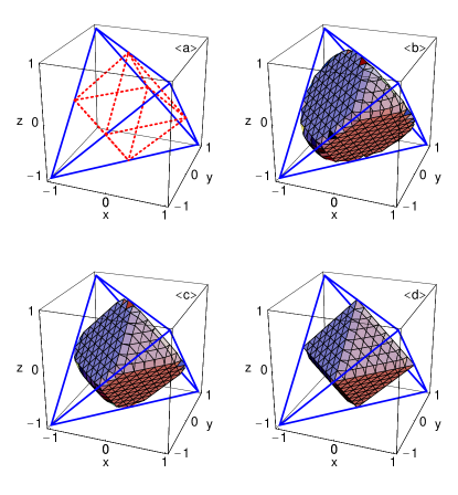
Figure 1: Investigation of the criterion from Eq. (26) for different values of $q:$ (a): The tetrahedron (blue, solid lines) of all states and the octahedron (red, dashed lines) which contains the separable states. (b): The subset of states which are not detected by Eq.(26) for $q=2.$ (c): As (b) but for $q=4.$ (d): As (b) but for $q=15.$

One can depict the border of the states which are not detected (for different $q$) in this three dimensional space. This has been done in Fig. 1. One can directly observe, that in the limit $q\rightarrow\infty$ the Corollary 1 enables one to detect all states, which are outside the octahedron. This is not by chance and can also be proven analytically: In the limit $q\rightarrow\infty$ Corollary 1 requires

$$\max_{i}\{p_{i}\in\mathcal{P}(M)_{\varrho}\}\leq\frac{1}{2}.$$ (27)

from a state to escape the detection. This condition is equivalent, to a set of four witnesses: The observables

$$\mathcal{W}_{i}=\frac{\mathbbm{1}}{2}-|BS_{i}\rangle\langle BS_{i}|$$ (28)

are all optimal witnesses, imposing the same condition on $\varrho$ witnesdef .

To investigate the consequences of Theorem 2, we focus on the case that the observables for Alice and Bob are spin measurements in the $x$,$y$, or $z$-direction. First note, that due to the Maassen-Uffink relation

$$S^{T}_{1}(\sigma_{x})_{\varrho}+S^{T}_{1}(\sigma_{y})_{\varrho}\geq\ln(2)$$ (29)

holds. This implies that for all separable states

$$S^{T}_{1}(\sigma_{x}\otimes\sigma_{x})_{\varrho}+S^{T}_{1}(\sigma_{y}\otimes\sigma_{y})_{\varrho}\geq\ln(2)$$ (30)

has to hold, too. This is just the bound which was numerically confirmed in giovannetti . Also the bound $S^{T}_{1}(\sigma_{x}\otimes\sigma_{x})_{\varrho}+S^{T}_{1}(\sigma_{y}\otimes\sigma_{y})_{\varrho}+S^{T}_{1}(\sigma_{z}\otimes\sigma_{z})_{\varrho}\geq 2\ln(2)$ for all separable states has been asserted in the same reference. In view of Theorem 2 this follows from the entropic uncertainty relation $S^{T}_{1}(\sigma_{x})_{\varrho}+S^{T}_{1}(\sigma_{y})_{\varrho}+S^{T}_{1}(\sigma_{z})_{\varrho}\geq 2\ln(2),$ proven in sanchez1 .

It is now interesting to take the Tsallis entropy and vary the parameter $q$. We do this numerically. We first compute by minimizing over all pure single qubit states

$$S_{xy}(q) = \min_{\varrho}(S^{T}_{q}(\sigma_{x})_{\varrho}+S^{T}_{q}(\sigma_{y})_{\varrho})$$

$$S_{xyz}(q) = \min_{\varrho}(S^{T}_{q}(\sigma_{x})_{\varrho}+S^{T}_{q}(\sigma_{y})_{\varrho}+S^{T}_{q}(\sigma_{z})_{\varrho}).$$

The results are shown in Fig. 2 analytical .

Figure 2: Numerical lower bounds in Eq. (LABEL:xyzschranke) depending on $q.$

Then we look at the corresponding separability criteria

$$S^{T}_{q}(\sigma_{x}\otimes\sigma_{x})+S^{T}_{q}(\sigma_{y}\otimes\sigma_{y})\geq S_{xy}(q)$$ (32)

$$S^{T}_{q}(\sigma_{x}\otimes\sigma_{x})+S^{T}_{q}(\sigma_{y}\otimes\sigma_{y})+S^{T}_{q}(\sigma_{z}\otimes\sigma_{z})\geq S_{xyz}(q)$$

(33)

To investigate the power of this criteria, let us look at Werner states $\rho(p)=p|\psi^{-}\rangle\langle\psi^{-}|+(1-p)\mathbbm{1}/4.$ We can make the following estimation: There are single qubit states with $\mathcal{P}(\sigma_{x})=\mathcal{P}(\sigma_{y})=\{(2-\sqrt{2})/4,(2+\sqrt{2})/4\}.$ The lower bound $S_{xy}(q)$ must therefore obey $S_{xy}(q)\leq 2S^{T}_{q}(\{(2-\sqrt{2})/4,(2+\sqrt{2})/4\}).$ For the Werner states we have $\mathcal{P}(\sigma_{x}\otimes\sigma_{x})=\mathcal{P}(\sigma_{y}\otimes\sigma_{y})=\{(1+p)/2,(1-p)/2\}.$ From this one can easily calculate that Eq. (32) cannot detect them for $p\leq 1/\sqrt{2}\approx 0.707.$ A similar argumentation shows that Eq. (33) has to fail for $p\leq 1/\sqrt{3}\approx 0.577.$ The numerical results are shown in Fig. 3. They show that indeed the Tsallis entropy for $q\in[2;3]$ can reach this bound.

Here, it is important to note that Werner states are already entangled for $p>1/3.$ The criteria from Eqns. (32,33) therefore fail to detect all Werner states, while the criterion from Eq. (27) is strong enough to detect all of them.

Figure 3: Values of $p_{min}$ depending on $q$ such that for $p>p_{min}$ Werner states of the form $\rho(p)=p|\psi^{-}\rangle\langle\psi^{-}|+(1-p)\mathbbm{1}/4.$ are detected via Eqns. (32,33). The curve $p_{xy}$ refers to the separability criterion in Eq. (32) and $p_{xyz}$ to Eq. (33). Note that Werner states are entangled for $p>1/3.$

As already mentioned, the Tsallis entropy is not the only entropic function. A more general function is of the type:

$$S^{RC}_{a,t}(\mathcal{P}) := \sum_{i}f(p_{i}),$$

$$f(x) := g_{t}(x-a)-(1-x)g_{t}(-a)-xg_{t}(1-a)$$

$$\mbox{ with }a\in[0;1],$$

$$g_{t}(y) := -\frac{\ln(\cosh(ty))}{2t}\mbox{ with }t\in[0;\infty).$$ (34)

One can show that $\mathcal{P}\succ\mathcal{Q}$ iff $S^{RC}_{a,t}(\mathcal{Q})\leq S^{RC}_{a,t}(\mathcal{P})$ for all $a$ and $t$ argentina2 . This is a property which does not hold for the Tsallis entropy. But this does not mean that criteria based on $S^{RC}_{a,t}$ are stronger than criteria based on the $S^{T}_{q}.$ With the use of the entropy $S^{RC}_{a,t}$ one can, of course, better use the property of Lemma 1. But since for the proof of Theorem 2 also the concavity of the entropy was used, one might loose this advantage there. In fact, by numerical calculations one can easily show that for $a=1/2$ and $t$ large the criterion using $S^{RC}_{a,t}$ and the measurements $\sigma_{x}\otimes\sigma_{x}$ and $\sigma_{y}\otimes\sigma_{y}$ (resp. $\sigma_{x}\otimes\sigma_{x},\sigma_{y}\otimes\sigma_{y}$ and $\sigma_{z}\otimes\sigma_{z}$) reaches, as the Tsallis entropy, the best possible value $p=1/\sqrt{2}.$ (resp. $p=1/\sqrt{3}$).

IV.2 Three qubits

Here we want to show with two examples how true multipartite entanglement can be detected. We focus on three qubit states. Let us first recall some facts about them duer1 ; acin :

Let us first consider pure states. There are two classes of pure states which are not genuine tripartite entangled: The fully separable states, which can be written as $|\phi_{fs}\rangle_{ABC}=|\alpha\rangle_{A}\otimes|\beta\rangle_{B}\otimes|\gamma\rangle_{C},$ and the biseparable states which are product states with respect to a certain bipartite splitting. One example is $|\phi_{bs}\rangle_{A-BC}=|\alpha\rangle_{A}\otimes|\delta\rangle_{BC}.$ There are three possibilities of grouping two qubits together, hence there are three classes of biseparable states. The genuine tripartite entangled states are the states which are neither fully separable nor biseparable. There are two classes of fully entangled states which are not convertible into each other by stochastic local operations and classical communication duer1 . These classes are called the GHZ-class and the W-class.

A mixed state is called fully separable if it can be written as a convex combination of fully separable pure states. A state is called biseparable if it can be written as a convex combination of biseparable pure states. Finally, a mixed state is fully entangled if it is neither biseparable nor fully separable. There are again two classes of fully entangled mixed states, the W-class (i.e. the states which can be written as a mixture of pure W-class states) and the GHZ-class. Also, it can be shown that the W-class forms a convex set inside the GHZ-class acin .

The results of Theorem 1 can easily be applied to multipartite systems:

Corollary 2. Let $M=\sum_{i}\mu_{i}|\psi_{i}\rangle\langle\psi_{i}|$ be an observable which is GHZ-diagonal, i.e. the $|\psi_{i}\rangle$ are of the form $|\psi_{1/5}\rangle=(|000\rangle\pm|111\rangle)/\sqrt{2};\;\;|\psi_{2/6}\rangle=(|100\rangle\pm|011\rangle)/\sqrt{2};\;\;|\psi_{3/7}\rangle=(|010\rangle\pm|101\rangle)/\sqrt{2};\;\;|\psi_{4/8}\rangle=(|001\rangle\pm|110\rangle)/\sqrt{2}.$ Then for all biseparable states

$$S^{T}_{q}(M)_{\varrho}\geq\frac{1-2^{1-q}}{q-1}$$ (35)

holds. For states belonging to the W-class the entropy is bounded by $S^{T}_{q}(M)_{\varrho}\geq({1-(3/4)^{q}+(1/4)^{q}})/({q-1}).$

Proof. Due to the concavity of the entropy we have to show the bound only for pure biseparable states. Then the proof follows directly from the fact that the maximal overlap between the states $|\psi_{i}\rangle$ and the biseparable (resp. W-class) states is $1/2$ (resp. $3/4$) acin ; wei . $\hfill\Box$

Again, as in the two qubit case, for $q=2$ the criterion is equivalent to a criterion in terms of variances guhne1 . Also one can show that this criterion becomes stronger, when $q$ increases, and in the limit $q\rightarrow\infty$ it is equivalent to a set of eight witnesses of the type $\mathcal{W}_{i}=1/2\cdot\mathbbm{1}-|\psi_{i}\rangle\langle\psi_{i}|$ (resp. $\mathcal{W}_{i}=3/4\cdot\mathbbm{1}-|\psi_{i}\rangle\langle\psi_{i}|$).

In order to show that also Theorem 2 can be applied for the detection of multipartite entanglement, we give an example which allows to detect the three qubit GHZ state.

Corollary 3. Let $\varrho$ be a biseparable three qubit state. Then for the Shannon entropy as well as for the Tsallis entropy for $q\in\{2,3,4,...\}$ the following bounds hold:

$$S^{T}_{1}(\sigma_{x}\otimes\sigma_{x}\otimes\sigma_{x})_{\varrho}+S^{T}_{1}(\sigma_{z}\otimes\sigma_{z}\otimes\mathbbm{1})_{\varrho}+S^{T}_{1}(\mathbbm{1}\otimes\sigma_{z}\otimes\sigma_{z})_{\varrho} \geq \ln(2)$$ (36)

$$S^{T}_{q}(\sigma_{x}\otimes\sigma_{x}\otimes\sigma_{x})_{\varrho}+S^{T}_{q}(\sigma_{z}\otimes\sigma_{z}\otimes\mathbbm{1})_{\varrho}+S^{T}_{q}(\mathbbm{1}\otimes\sigma_{z}\otimes\sigma_{z})_{\varrho} \geq \frac{1-2^{1-q}}{q-1}$$ (37)

For the GHZ state $|GHZ\rangle=(|000\rangle+|111\rangle)/\sqrt{2}$ the left hand side of Eqns. (36, 37) is zero.

Proof. Again, we only have to prove the bound for pure biseparable states. If a state is A-BC biseparable, the bounds in Eq. (36) follows directly from Theorem 2 and the Maassen Uffink uncertainty relation, which guarantees that for the first qubit $S^{T}_{1}(\sigma_{x})+S^{T}_{1}(\sigma_{z})+S^{T}_{1}(\mathbbm{1})\geq\ln(2)$ holds. Eq. (37) follows similarly, using the fact that $S^{T}_{q}(\sigma_{x})+S^{T}_{q}(\sigma_{z})\geq{(1-2^{1-q})}/{(q-1)}$ analytical . The proof for the other bipartite splittings is similar. $\hfill\Box$

Note that the observables used in Corollary 3 are so called stabilizers of the GHZ state. By this we mean that the GHZ state is an eigenstate of them with the eigenvalue one. Stabilizers can also be used to detect the entanglement of other multipartite entangled states toth ; toth2 .

Let us finally investigate, how robust against noise these criteria are. One can easily calculate that a state of the type $\varrho(p)=p|GHZ\rangle\langle GHZ|+(1-p)\mathbbm{1}/8$ can be detected by Eq. (36) if $p\geq 0.877.$ Eq. (37) seems to detect the most states for $q\in\{2,3\},$ then they detect $\varrho(p)$ for $p\geq\sqrt{2/3}\approx 0.816.$

V Conclusion

In conclusion, we have established connections between entropic uncertainty relations and entanglement. We have presented two methods to develop entropy based separability criteria. Especially we have shown how an arbitrary entropic uncertainty relation on one part of a composite quantum system can be used to detect entanglement in the composite system. We have investigated the power of these criteria and have shown that they are extendible to multipartite systems.

There are several question which should be addressed further. One interesting question is, which entropies are best suited for special detection problems. We have seen that in some of our examples the Tsallis entropies with $q\in[2;3]$ seemed to be the best. Clarifying the physical meaning of the parameter $q$ might help to understand this property.

Another important task is to find good (i.e. sharp) entropic uncertainty relations, especially for more than two observables. One the one hand, this is an interesting field of study for itself, on the other hand, this might help to explore the full power of the methods presented here. Finally, it is worth mentioning, that entropic uncertainty relations also enable a new possibility of locking classical correlation in quantum states datahiding . A better understanding of entropic uncertainty relations would therefore also lead to a better understanding of this phenomenon.

VI Acknowledgements

We wish to thank Dagmar Bruß, Michał, Paweł and Ryszard Horodecki, Philipp Hyllus, Anna Sanpera, Geza Tóth and Michael Wolf for discussions.

This work has been supported by the DFG (Graduiertenkolleg “Quantenfeldtheoretische Methoden in der Teilchenphysik, Gravitation, Statistischen Physik und Quantenoptik” and Schwerpunkt “Quanten-Informationsverarbeitung”).

References

- (1) W. Heisenberg, Z. Phys. 43, 172 (1927).
- (2) H.P. Robertson, Phys. Rev. 34, 163 (1929); ibid. 46 794 (1934).
- (3) I. Białynicki-Birula and J. Mycielski, Commun. Math. Phys. 44, 129 (1975). D. Deutsch, Phys. Rev. Lett. 50, 631 (1983); K. Kraus, Phys. Rev. D 35, 3070 (1987).
- (4) H. Maassen and J.B.M. Uffink, Phys. Rev. Lett. 60, 1103, (1988); see also H. Maassen, in “Quantum Probability and Applications V”, Lecture Notes in Mathematics 1442, edited by L. Accardi, W. von Waldenfels, (Springer, Berlin, 1988) p. 263.
- (5) E. Schrödinger, Naturwissenschaften 23, 807 (1935); 23, 823 (1935); 23, 844 (1935); A. Einstein, N. Podolski, and N. Rosen, Phys. Rev. 47, 777 (1935).
- (6) A.K. Ekert, Phys. Rev. Lett. 67, 661 (1991); C.H. Bennett, G. Brassard, C. Crépeau, R. Jozsa, A. Peres and W.K. Wootters, Phys. Rev. Lett. 70, 1895 (1993).
- (7) For recent results on the separability problem see A.C. Doherty, P.A. Parrilo, and F.M. Spedalieri, Phys. Rev. Lett. 88, 187904 (2002); O. Rudolph, Phys. Rev. A 67, 032312 (2003); K. Chen and L. Wu, Quant. Inf. Comp. 3, 193 (2003); M. Horodecki, P. Horodecki, and R. Horodecki, quant-ph/0206008; A.C. Doherty, P.A. Parrilo, and F.M. Spedalieri, Phys. Rev. A 69, 022308 (2004); for a review see D. Bruß, J. I. Cirac, P. Horodecki, F. Hulpke, B. Kraus, M. Lewenstein, and A. Sanpera, J. Mod. Opt. 49, 1399 (2002).
- (8) M.D. Reid and P.D. Drummond, Phys. Rev. Lett. 60, 2731 (1988); L.-M. Duan, G. Giedke, J. I. Cirac, and P. Zoller, ibid. 84, 2722 (2000); S. Mancini, V. Giovannetti, D. Vitali, and P. Tombesi, ibid. 88, 120401 (2002); P. van Loock and A. Furusawa, Phys. Rev. A 67, 052315 (2003); G. Tóth, C. Simon, and J.I. Cirac, ibid. 68, 062310 (2003).
- (9) H.F. Hofmann and S. Takeuchi, Phys. Rev. A 68, 032103 (2003); H.F. Hofmann, ibid. 68, 034307 (2003).
- (10) O. Gühne, Phys. Rev. Lett. 92, 117903 (2004).
- (11) G. Tóth, Phys. Rev. A 69, 052327 (2004).
- (12) R. Horodecki and P. Horodecki, Phys. Lett. A 194, 147, (1994).
- (13) V. Giovannetti, Phys. Rev. A 70, 012102 (2004).
- (14) See, e.g. R. Horodecki, P. Horodecki, and M. Horodecki, Phys. Lett. A 210, 377, (1996); R. Horodecki and M. Horodecki, Phys. Rev. A 54, 1838, (1996); N.J. Cerf and C. Adami, Phys. Rev. Lett. 79, 5194 (1997); A. Vidiella-Barranco, Phys. Lett A 260, 335 (1999); S. Abe and A.K. Rajagopal, Physica A 289, 157 (2001); C. Tsallis, S. Lloyd, and M. Baranger Phys. Rev. A 63, 042104 (2001); K.G.H. Vollbrecht, and M.M. Wolf, J. Math. Phys. 43, 4299 (2002); F. Mintert and K. Życzkowski, Phys. Rev. A 69, 022317 (2004); some of these results follow from a majorization relation proved in: M.A. Nielsen and J. Kempe, Phys. Rev. Lett. 86, 5184 (2001).
- (15) C. Shannon and W. Weaver, The Mathematical Theory of Communication. (University of Illinois, Urbana, 1949).
- (16) J. Havrda and F. Charvat, Kybernetika 3, 30 (1967).
- (17) C. Tsallis, J. Stat. Phys. 52, 479 (1988).
- (18) A. Rényi, Valószínűségszámítás, (Tankönyvkiadó, Budapest, 1966). English translation: Probability theory, (North Holland, Amsterdam, 1970).
- (19) A. Wehrl, Rev. Mod. Phys. 50, 221 (1978); for results on the relationships between the different entropies see also K. Życzkowski, Open Syst. Inf. Dyn. 10, 297 (2003).
- (20) Note that the sign “” is sometimes defined the other way round in the literature.
- (21) N. Canosa and R. Rossignoli, Phys. Rev. Lett. 88, 170401 (2002); R. Rossignoli and N. Canosa, Phys. Rev. A 66, 042306 (2002).
- (22) R. Rossignoli and N. Canosa, Phys. Rev. A 67, 042302 (2003).
- (23) M. Krishna and K.R. Parthasarathy, Sankhya: The Indian Journal of Statistics, Series A, 64, 842 (2002).
- (24) J. Sánchez, Phys. Lett. A 173, 233 (1993).
- (25) V. Majerník and E. Majerníková, Rep. Math. Phys. 47, 381 (2001).
- (26) J. Sánchez-Ruiz, Phys. Lett. A 244, 189 (1998).
- (27) G.-C. Ghirardi, L. Marinatto, and R. Romano, Phys. Lett. A 317, 32 (2003).
- (28) T.-C. Wei and P.M. Goldbart, Phys. Rev. A 68, 042307 (2003); M. Bourennane, M. Eibl, C. Kurtsiefer, S. Gaertner, H.Weinfurter, O. Gühne, P. Hyllus, D. Bruß, M. Lewenstein, and A. Sanpera, Phys. Rev. Lett. 92, 087902 (2004).
- (29) R. Bhatia, Matrix analysis, (Springer, Berlin, 1997).
- (30) This geometrical picture was also studied in R. Horodecki and M. Horodecki, Phys. Rev. A 54, 1838, (1996); R.A. Bertlmann, H. Narnhofer, and W. Thirring, ibid. 66, 032319 (2002).
- (31) An entanglement witness is an observable with the property for all separable states and for some entangled states. See, e.g. M. Lewenstein, B. Kraus, J.I. Cirac, and P. Horodecki, Phys. Rev. A 62, 052310 (2000).
-
(32)
Some bounds for this figure can also
be proven analytically:
For one can prove
The proof goes as follows: It is clear that the mimimum of is obtained for a state in the - plane. Calculating for a pure state in this plane one recognizes that minimizing is equivalent to maximizing Using now the formula(38)
(see E.T. Whittaker and G.N. Watson, A Course of Modern Analysis (Cambridge University Press, 1927), p. 263) one can rewrite as a series of the form Then it is easy to show that if for all the coefficients are positive, thus is maximized if This proves that is minimized for an eigenstate of which yields (38). Numerically, (38) seems also to hold for other values of except(39) - (33) W. Dür, G. Vidal, and J.I. Cirac, Phys. Rev. A, 62, 062314 (2000).
- (34) A. Acín, D. Bruß, M. Lewenstein, and A. Sanpera, Phys. Rev. Lett. 87, 040401 (2001).
- (35) G. Tóth, (private communication); see also V. Scarani, A. Acín, E. Schenck, and M. Aspelmeyer, quant-ph/0405119; G. Tóth and O. Gühne, quant-ph/0405165.
- (36) D.P. DiVincenzo, M. Horodecki, D.W. Leung, J.A. Smolin, and B.M. Terhal, Phys. Rev. Lett. 92, 067902 (2004); P. Hayden, D.W. Leung, P.W. Shor, and A. Winter, quant-ph/0307104.