Control of decoherence: analysis and comparison of three different strategies

Abstract

We analyze and compare three different strategies, all aimed at controlling and eventually halting decoherence. The first strategy hinges upon the quantum Zeno effect, the second makes use of frequent unitary interruptions (“bang-bang” pulses and their generalization, quantum dynamical decoupling), and the third of a strong, continuous coupling. Decoherence is shown to be suppressed only if the frequency $N$ of the measurements/pulses is large enough or if the coupling $K$ is sufficiently strong. Otherwise, if $N$ or $K$ are large, but not extremely large, all these control procedures accelerate decoherence. We investigate the problem in a general setting and then consider some practical examples, relevant for quantum computation.

I Introduction

Interactions with the environment deteriorate the purity of quantum states. This general phenomenon, known as decoherence decoherencereview , is a serious obstacle against the preservation of quantum superpositions and entanglement over long periods of time. Decoherence entails non-unitary evolutions, with serious consequences, like a loss of information and/or probability leakage towards the environment.

This issue is recently attracting much attention in view of interesting applications: for instance, the possibility of controlling and eventually halting decoherence is a key problem in quantum computation Review , where several computational states are simultaneously described by a single wave function and parallel information processing is carried out by unitary operations. In such a situation, efficient quantum algorithms need large scale computations, performed over (microscopically) long time spans Unruh .

A number of interesting schemes have been proposed during the last few years in order to counter the effects of decoherence. Among these, there are quantum error correcting codes ErrorCorrecting , schemes based on feedback or stochastic control feedback , the use of decoherence free subspaces and noiseless subsystems NoiselessSub and mechanisms based on “bang-bang” (BB) pulses and their generalization, quantum dynamical decoupling BBDDsem ; BBDD ; Zanardi ; Vitali ; BL . In this context, it was recently proposed bang that the method of dynamical decoupling can be unified with the basic ideas underlying the quantum Zeno effect (QZE) QZEseminal ; MS (for a review, see QZEreview ; PIO ). In particular, the decoherence free subspace is one of the dynamically generated quantum Zeno subspaces FPsuper , within which the dynamics is not trivial compactregularize and whose subtle mathematical aspects are still debated Friedman72 ; MS ; Gustavson ; ExnerIchinose ; Schmidt ; MisraAntoniou .

It is worth stressing that the “bang-bang” scheme is a well-established “classical” control method, typically used in engineering problems and in connection with spin-echo techniques: see, for instance, Ref. classicalBB . Its revival in quantum-information-related problems is only very recent. The key ingredient of BB and dynamical decoupling is to apply frequent (unitary) interruptions during the evolution of the system, in order to suppress the system-environment interaction. The similarity with the QZE was already noticed in BBDDsem . It is however clear that the two procedures are physically equivalent, if one adheres to the commonly accepted interpretation of the QZE as a bona fide dynamical process, that can be completely explained in terms of unitary evolutions QZEbxl . One should notice that this idea hinges upon a seminal remark by Wigner Wigner63 , who introduced in 1963 the notion of “spectral decomposition,” namely a dynamical process that associates a different wave packet with each eigenvalue of the observable to be measured. For example, the interesting proposal by Cook Cook and the subsequent experiment with Rabi oscillations WinelandZeno can be easily interpreted in fully dynamical terms when one observes that the “measurement” was realized as a dynamical process (optical pulse irradiation) PIO ; QZEbxl ; Itanodisc .

Once this physical equivalence is appreciated, the next logical step is a natural one: after having analyzed and understood the consequences of frequent unitary pulses, one studies the effect of a strong (unitary) continuous coupling. The relationship between these two procedures can be made mathematically precise (see Sec. II) and is of interest in itself: if an external field or “apparatus” is coupled to the system in such a way that the state of the system is “monitored” in some sense Simonius ; HS ; Peres ; Schulman98 , a Zeno-like dynamics takes place in the strong coupling limit and once again one can tailor decoherence-free subspaces bang . This happens to be one of the most efficient and convenient control procedures, from a practical point of view.

The aim of this article is to investigate these different physical procedures (Zeno, BB-dynamical decoupling and continuous coupling) and compare their effects. We will study the dynamics generated by very frequent interruptions (projective measurements or unitary “kicks,” yielding dynamical decoupling), or by very strong coupling, and investigate the possibility of designing decoherence-free subspaces. The method is general and can be applied to diverse situations of practical interest, such as atoms and ions in cavities, organic molecules, quantum dots and Josephson junctions Wineland ; expt ; qdot ; JJs .

Our main objective is to endeavor to understand whether it is possible to control decoherence Calarco ; Falci ; Paladino:02 ; Falci:03 ; KofKu . Clearly, this requires a thorough understanding of the physical mechanisms that provoke decoherence and in general dissipative phenomena. One finds that very frequent kicks/measurements or very strong couplings can indeed control the evolution of the system and suppress decoherence. The physical mechanisms at the origin of this phenomenon are very close to the quantum Zeno effect. However, if the kicks/measurements are not extremely frequent or the coupling not extremely strong, both controls may accelerate decoherence. This extends the notion of “inverse” quantum Zeno effect (IZE) IZE ; Heraclitus to a wider framework (not necessarily based on projection operators and non-unitary dynamics) and entails a deterioration of the performance of these schemes. We will analyze this effect in great detail and see that in order to avoid it, one must carefully design the control and study the timescales involved. Our analysis is of general validity; however, for the sake of definiteness, we will study in particular the control of thermal decoherence TTFP .

This article is organized as follows. In Sec. II we briefly review the main features of the different control procedures. Our analysis is based on a master equation which is derived in Sec. III, where the relevant timescales are emphasized and the general type of interaction specified. We then consider the case of thermal decoherence, discussing the Zeno control, the control via dynamical decoupling and the control by means of a strong continuous coupling in Secs. IV, V and VI, respectively. Some relevant examples are then considered in Sec. VII, where we focus on the primary role of the form factors of the interaction in order to compare the different control procedures. Section VIII is devoted to conclusions and perspectives.

II Control procedures: generalities

Let the total system consist of a target system and a reservoir and its Hilbert space ${\cal H}_{\rm tot}={\cal H}_{S}\otimes{\cal H}_{B}$ be expressed as the tensor product of the system Hilbert space ${\cal H}_{S}$ and the reservoir Hilbert space ${\cal H}_{B}$. The total Hamiltonian

$$H_{\rm tot}=H_{0}+H_{SB}=H_{S}\otimes\openone_{B}+\openone_{S}\otimes H_{B}+H_{SB}$$ (1)

is the sum of the system Hamiltonian $H_{S}\otimes\openone_{B}$, the reservoir Hamiltonian $\openone_{S}\otimes H_{B}$ and their interaction $H_{SB}$, which is responsible for decoherence; the operators $\openone_{S}$ and $\openone_{B}$ are the identity operators in the Hilbert spaces ${\cal H}_{S}$ and ${\cal H}_{B}$, respectively, and the operators $H_{S}$ and $H_{B}$ act on ${\cal H}_{S}$ and ${\cal H}_{B}$, respectively.

The dynamics of the total system is conveniently expressed in terms of the Liouville operator (Liouvillian) ${\cal L}_{\rm tot}$, defined by

$${\cal L}_{\mathrm{tot}}\rho\equiv-i[H_{\rm tot},\rho]=-i\left(H_{\rm tot}\rho-\rho H_{\rm tot}\right)\ ,$$ (2)

where $\rho$ is the density matrix. If the Hamiltonian is given by (1), the Liouvillian is accordingly decomposed into

$${\mathcal{L}}_{\mathrm{tot}}={\mathcal{L}}_{0}+{\mathcal{L}}_{SB}={\mathcal{L}}_{S}+{\mathcal{L}}_{B}+{\mathcal{L}}_{SB},$$ (3)

where the meaning of the symbols is obvious. We will not explicitly write the coupling constant $\lambda$ multiplying the interaction Liouvillian ${\mathcal{L}}_{SB}$.

We focus on a proper subspace ${\cal H}_{\rm comp}\subset{\cal H}_{S}$, in which quantum computation is to be performed. For this reason we will look in detail at the case

$${\cal H}_{S}={\cal H}_{\rm comp}\oplus{\cal H}_{\rm orth}.$$ (4)

In particular, when we will look at some concrete examples, in Sec. VII, the computation subspace will be a qubit, ${\cal H}_{\rm comp}=\mathbb{C}^{2}$.

Since, in general, the reservoir state is mixed, it is convenient to describe the time evolution in terms of density matrices. In the case of a quantum state manipulation, the initial state of the total system $\rho(0)$ is set to be a tensor product of the system initial state $\sigma(0)$ and a reservoir (usually equilibrium) state $\rho_{B}$

$$\rho(0)=\sigma(0)\otimes\rho_{B}.$$ (5)

The validity of this assumption, usually taken for granted, is discussed in Appendix A (see also factorassumption ). The system state $\sigma(t)$ at time $t$ is given by the partial trace of the state $\rho(t)$ of the whole system with respect to the reservoir degrees of freedom:

$$\sigma(t)\equiv{\rm tr}_{B}\rho(t).$$ (6)

When $\sigma(t)$ is not unitarily equivalent to $\sigma(0)$ for a given class of initial states, decoherence is said to occur. The purpose of the control is to suppress such decoherence. Note that, for the control of decoherence, it is not necessary to look at all possible states: rather, it is sufficient to consider only those initial states which are relevant to the quantum state manipulation in question.

II.1 Quantum Zeno control

We first look at the Zeno control, by adapting the argument of Ref. FPsuper . The control is obtained by performing frequent measurements of the system. The measurement is described by a projection superoperator $\hat{P}$ acting on the density matrix

$$\rho\to{\hat{P}}\rho\equiv\sum_{n}\left(P_{n}\otimes\openone_{B}\right)\rho\left(P_{n}\otimes\openone_{B}\right),$$ (7)

where $\{P_{n}\}$ is a set of orthogonal projection operators acting on ${\cal H}_{S}$. In the following, we restrict our analysis to a measuring apparatus that does not “select” the different outcomes (nonselective measurement) Schwinger , with a complete set of projection operators $\sum_{n}P_{n}=\openone_{S}$. The measurement is designed so that

$${\hat{P}}H_{SB}=\sum_{n}\left(P_{n}\otimes\openone_{B}\right)H_{SB}\left(P_{n}\otimes\openone_{B}\right)=0.$$ (8)

In terms of the Liouvillian, this condition reads

$${\hat{P}}{\mathcal{L}}_{SB}{\hat{P}}=0.$$ (9)

(We will see in the next subsection that a similar requirement is necessary for the BB control and for the control via a continuous coupling.) The Zeno control consists in performing repeated nonselective measurements at times $t=k\tau$ ($k=0,1,2,\ldots$) (we include an initial “state preparation” at $t=0$). Between successive measurements, the system evolves via $H_{\rm tot}$. The density matrix after $N+1$ measurements, with an initial state $\rho(0)$, is given by

$$\rho(t)=\rho(N\tau)=\left({\hat{P}}e^{{\mathcal{L}}_{\rm tot}\tau}{\hat{P}}\right)^{N}\rho(0)\ .$$ (10)

We take the limit $\tau\to 0$ while keeping $t=N\tau$ constant and get

$$\rho(t)={\hat{P}}\left[1+{\hat{P}}{\cal L}_{\rm tot}{\hat{P}}\tau+{\rm O}\left(\tau^{2}\right)\right]^{t\over\tau}\rho(0)\stackrel{{\scriptstyle\tau\to 0}}{{\longrightarrow}}{\hat{P}}e^{{\hat{P}}{\cal L}_{\rm tot}{\hat{P}}t}\rho(0)\ .$$ (11)

Equation (8) yields ${\hat{P}}{\cal L}_{\rm tot}{\hat{P}}\rho=-i{\hat{P}}[H_{\rm tot},{\hat{P}}\rho]=-i{\hat{P}}[({\hat{P}}H_{\rm tot}),\rho]=-i{\hat{P}}[H^{\prime}_{S}\otimes\openone_{B}+\openone_{S}\otimes H_{B},\rho]$ , whence

$${\hat{P}}e^{{\hat{P}}{\cal L}_{\rm tot}{\hat{P}}t}\rho(0) = {\hat{P}}e^{{\cal L}_{\rm tot}^{\prime}t}\rho(0)$$ (12)

$$= {\hat{P}}\left(e^{-iH^{\prime}_{\rm tot}t}\rho(0)e^{iH^{\prime}_{\rm tot}t}\right)$$

$$= {\hat{P}}\left(e^{-iH^{\prime}_{S}t}\otimes e^{-iH_{B}t}\rho(0)e^{iH^{\prime}_{S}t}\otimes e^{iH_{B}t}\right)\ ,$$

where the controlled Hamiltonian $H^{\prime}_{\rm tot}$ and Liouvillian ${\mathcal{L}}^{\prime}_{\rm tot}$ are given by

$$H^{\prime}_{\rm tot} \equiv {\hat{P}}H_{\rm tot}=\sum_{n}\left(P_{n}\otimes\openone_{B}\right)H_{\rm tot}\left(P_{n}\otimes\openone_{B}\right)=H^{\prime}_{S}\otimes\openone_{B}+\openone_{S}\otimes H_{B}\ ,$$ (13)

$${\mathcal{L}}^{\prime}_{\rm tot} = {\hat{P}}{\cal L}_{\rm tot}{\hat{P}}={\hat{P}}{\cal L}_{S}{\hat{P}}+{\mathcal{L}}_{B}{\hat{P}}={\mathcal{L}}^{\prime}_{S}+{\mathcal{L}}_{B}{\hat{P}}\ .$$ (14)

with $H^{\prime}_{S}={\hat{P}}H_{S}=\sum_{n}P_{n}H_{S}P_{n}$. Hence, as a result of infinitely frequent measurements, the system-reservoir coupling is eliminated and, thus, decoherence is halted. We notice the formation of invariant Zeno subspaces FPsuper : in the limit of very frequent measurements, the evolution is given by (13)-(14) and transitions among different sectors of the Hilbert space vanish, yielding a superselection rule. The subspaces are defined by the superoperator $\hat{P}$ defining the measurement. The “decoherence-free” subspace is one of these Zeno subspaces.

We will assume for simplicity that ${\hat{P}}$ commutes with the system Liouvillian

$${\hat{P}}{\mathcal{L}}_{S}={\mathcal{L}}_{S}{\hat{P}},$$ (15)

i.e. $H^{\prime}_{S}={\hat{P}}H_{S}=H_{S}$, because our purpose is to control decoherence and we are not interested in a QZE over the system Hamiltonian $H_{S}$. The above assumption is equivalent to the following hypothesis on the Hamiltonian

$$\left[P_{n},H_{S}\right]=0,\qquad\forall n\ .$$ (16)

In such a case

$${\mathcal{L}}^{\prime}_{\rm tot}=({\mathcal{L}}_{S}+{\mathcal{L}}_{B}){\hat{P}}\ .$$ (17)

II.2 Control via Quantum Dynamical Decoupling and “Bang-Bang” Pulses

We now turn our attention to the so-called quantum dynamical decoupling BBDD ; Zanardi ; Vitali , of which “bang-bang” pulses can be viewed as a particular case. The control of decoherence is achieved via a time-dependent system Hamiltonian $H_{c}(t)$:

$$H(t)=H_{\rm tot}+H_{c}(t)\otimes\openone_{B}\ ,$$ (18)

where $H_{c}(t)$ is designed so that $U_{c}(t)\equiv{\cal T}\exp\left(-i\int_{0}^{t}H_{c}(s)ds\right)$ (${\cal T}$ denotes time ordering) satisfies

$$U_{c}(t+\tau)=U_{c}(t)$$ (19)

$$\int_{0}^{\tau}dt\bigl{(}U_{c}^{\dagger}(t)\otimes\openone_{B}\bigr{)}H_{SB}\bigl{(}U_{c}(t)\otimes\openone_{B}\bigr{)}=0.$$ (20)

In the interaction picture in which $H_{c}(t)$ is unperturbed, the density matrix at time $t=N\tau$, with initial state $\rho(0)$, is given by $\rho(t)=U_{\rm tot}(N\tau)\rho(0)U_{\rm tot}^{\dagger}(N\tau)$ where

$$U_{\rm tot}(N\tau)={\cal T}\exp\left(-i\int_{0}^{N\tau}{\widetilde{H}}_{\rm tot}(s)ds\right)=\left[{\cal T}\exp\left(-i\int_{0}^{\tau}{\widetilde{H}}_{\rm tot}(s)ds\right)\right]^{N}$$ (21)

and ${\widetilde{H}}_{\rm tot}(t)=\bigl{(}U_{c}^{\dagger}(t)\otimes\openone_{B}\bigr{)}H_{\rm tot}\bigl{(}U_{c}(t)\otimes\openone_{B}\bigr{)}$. The second equality follows from the periodicity of ${\widetilde{H}}_{\rm tot}(t)$. A standard Magnus expansion of the time-ordered exponential Magnus leads to

$${\cal T}\exp\left(-i\int_{0}^{\tau}{\widetilde{H}}_{\rm tot}(s)ds\right)=e^{-i[{\bar{H}}^{(0)}+{\bar{H}}^{(1)}+\cdots]\tau}$$ (22)

where ${\bar{H}}^{(0)}\equiv{1\over\tau}\int_{0}^{\tau}{\tilde{H}}_{\rm tot}(s)ds$ and the term ${\bar{H}}^{(j)}$ is of order $\tau^{j}$ ($j=1,2,\cdots$). By assumption (20), one has

$${\bar{H}}^{(0)}=H^{\prime}_{S}\otimes\openone_{B}+\openone_{S}\otimes H_{B}=H^{\prime}_{\rm tot}\ ,$$ (23)

which is formally identical to (13), where $H^{\prime}_{S}\equiv{1\over\tau}\int_{0}^{\tau}dtU_{c}^{\dagger}(t)H_{S}U_{c}(t)=\int_{0}^{1}dxU_{c}^{\dagger}(x\tau)H_{S}U_{c}(x\tau)$ is independent of $\tau$ because $U_{c}(t)$ is $\tau$-periodic by (19) and is always written as a function of $t/\tau$: $U_{c}(t)=V(t/\tau)$. Therefore, in the limit $\tau\to 0$ while keeping $t=N\tau$ constant, one obtains

$$U_{\rm tot}(t)=\left[1-iH^{\prime}_{\rm tot}\tau+{\rm O}\left(\tau^{2}\right)\right]^{t\over\tau}\stackrel{{\scriptstyle\tau\to 0}}{{\longrightarrow}}e^{-iH^{\prime}_{\rm tot}t}=e^{-iH^{\prime}_{S}t}\otimes e^{-iH_{B}t}\ .$$ (24)

In short, as a result of the infinitely fast control, the system-reservoir coupling is eliminated and, thus, decoherence is halted. As we shall see in a while, this is a consequence of the formation of invariant subspaces.

As is well known, dynamical decoupling is a generalization of the evolution obtained by acting on the system with “bang-bang” pulses BBDD . In the latter, particular case, one applies during a time interval $\tau$ two instantaneous unitary operators $U_{\mathrm{k}}$ and $U_{\mathrm{k}}^{\dagger}$ and gets bang

$$H^{\prime}_{\rm tot}={\hat{P}}H_{\rm tot}=\sum_{n}\left(P_{n}\otimes\openone_{B}\right)H_{\rm tot}\left(P_{n}\otimes\openone_{B}\right)$$ (25)

[see (13)], where the projections $P_{n}$ arise from the spectral decomposition

$$U_{\mathrm{k}}=\sum_{n}e^{-i\lambda_{n}}P_{n},\qquad(\lambda_{n}\neq\lambda_{m}\;\mathrm{mod}\;2\pi,\quad\mbox{for}\;n\neq m)\ .$$ (26)

Notice that the map ${\hat{P}}$ is in this case the projection onto the commutant

$$Z(U_{\mathrm{k}})=\{X|\;[X,U_{\mathrm{k}}]=0\}.$$ (27)

Equation (25) yields a convenient explicit expression of the effective Hamiltonian. As in the case discussed in the previous subsection, one observes the formation of invariant Zeno subspaces: transitions among different subspaces vanish in the $\tau\to 0$ limit, yielding a superselection rule. In this case, the subspaces are defined by (25)-(26) and are nothing but the ergodic sectors of $U_{\mathrm{k}}$.

By assuming again, as in (15)-(16), that ${\hat{P}}H_{S}=H_{S}$ and that ${\hat{P}}H_{SB}=0$, as in (8)-(9), we get that the controlled evolution for $\tau\to 0$ is given by

$$U_{\rm tot}(t)=e^{-iH^{\prime}_{\rm tot}t}=e^{-iH_{S}t}\otimes e^{-iH_{B}t}$$ (28)

or, in terms of Liouvillians, by $e^{{\mathcal{L}}^{\prime}_{\rm tot}t}$ with ${\mathcal{L}}^{\prime}_{\rm tot}={\hat{P}}{\mathcal{L}}_{\rm tot}{\hat{P}}=({\mathcal{L}}_{S}+{\mathcal{L}}_{B}){\hat{P}}$, exactly as in (17).

Moreover, in Ref. bang it was shown that one can obtain the same result (25) by repeating a single “bang”, i.e. by using a single instantaneous unitary operator $U_{\mathrm{k}}$, without closing the group with $U_{\mathrm{k}}^{\dagger}$. For simplicity, in the following we will always consider such a situation and will assume the commutation property (15). In such a case, the evolution is conveniently expressed in terms of the Liouvillian and density matrix

$$\rho(t)=\left[e^{{\mathcal{L}}_{\mathrm{k}}}e^{{\cal L}_{\rm tot}\tau}\right]^{\frac{t}{\tau}}{\hat{P}}\rho(0)\to e^{{\mathcal{L}}^{\prime}_{\mathrm{tot}}t}{\hat{P}}\rho(0),\qquad\tau\to 0\ ,$$ (29)

where ${\mathcal{L}}_{\mathrm{k}}$ is the Liouvillian corresponding to the evolution (26) and ${\mathcal{L}}^{\prime}_{\rm tot}$ is given by (17). Note that the controlled Hamiltonians for bang bang pulses, (25), and for the Zeno control, (13), coincide when the set of orthogonal projections (7) is chosen equal to the set (26) of eigenprojections of $U_{\rm k}$, namely

$${\mathcal{L}}_{\mathrm{k}}{\hat{P}}=0,\qquad({\hat{P}}\openone)=\openone.$$ (30)

Therefore, the two controls are equivalent in the ideal (limiting) case bang . However, throughout this article, by dynamical decoupling we will refer to a situation where the evolution is coherent (unitary), while by Zeno control to a situation where the evolution involves incoherent (nonunitary) processes, such as quantum measurements.

The index “$\mathrm{k}$” in the above expressions stands for “kicks.” In the following, we shall use the expressions “bang-bang” pulses and “kicks” interchangeably. The latter is reminiscent of quantum chaos qch1 . In fact, there is an interesting link between quantum chaotic dynamics, quantum diffusion processes and (inverse) quantum Zeno effect qch2 . We will not elaborate on this issue in the present article.

II.3 Control via a strong continuous coupling

The formulation in the preceding sections hinges upon instantaneous processes, that can be unitary or nonunitary. However, as explained in the Introduction, the basic features of the QZE can be obtained by making use of a continuous coupling, when the external system takes a sort of steady “gaze” at the system of interest. The mathematical formulation of this idea is contained in a theorem FPsuper on the (large-$K$) dynamical evolution governed by a generic Hamiltonian of the type

$$H_{K}=H_{\mathrm{tot}}+KH_{\mathrm{c}}\otimes\openone_{B},$$ (31)

which again need not describe a bona fide measurement process: $H_{\mathrm{c}}$ can be viewed as an “additional” interaction Hamiltonian performing the “measurement” and $K$ is a coupling constant.

Consider the time evolution operator

$$U_{K}(t)=\exp(-iH_{K}t).$$ (32)

In the infinitely strong measurement (infinitely quick detector) limit $K\to\infty$, the dominant contribution is $\exp(-iKH_{\mathrm{c}}t)$. One therefore considers the limiting evolution operator

$${\mathcal{U}}(t)=\lim_{K\to\infty}\exp(iKH_{\mathrm{c}}t)\,U_{K}(t),$$ (33)

that can be shown to have the form

$${\mathcal{U}}(t)=\exp(-iH^{\prime}_{\mathrm{tot}}t),$$ (34)

where

$$H^{\prime}_{\mathrm{tot}}=\hat{P}H_{\mathrm{tot}}=\sum_{n}(P_{n}\otimes\openone_{B})H_{\mathrm{tot}}(P_{n}\otimes\openone_{B})\ ,$$ (35)

$P_{n}$ being the eigenprojection of $H_{\mathrm{c}}$ belonging to the eigenvalue $\eta_{n}$

$$H_{\mathrm{c}}=\sum_{n}\eta_{n}P_{n},\qquad(\eta_{n}\neq\eta_{m},\quad\mbox{for}\;n\neq m)\ .$$ (36)

By designing $H_{c}$ so that $\hat{P}H_{SB}=0$, the system-reservoir coupling is eliminated and, thus, decoherence is halted. Equation (35), restricted to the system of interest, is formally identical to (25) and (13).

In conclusion, the limiting evolution operator is

$$U_{K}(t)\sim\exp(-iKH_{\mathrm{c}}t)\,{\mathcal{U}}(t)=\exp\left(-iKt\sum_{n}\eta_{n}P_{n}\otimes\openone_{B}-i\hat{P}H_{\mathrm{tot}}t\right).$$ (37)

The above statements can be proved by making use of the adiabatic theorem Messiah61 . It is worth noting that the evolution in the strong coupling limit is known to force the system to “cling” to the eigenstates of the interaction Frasca . In this sense, one expects that the dynamics be dominated by $H_{\mathrm{c}}$ for $K$ large. The above theorem clarifies how the structure of $H_{\mathrm{c}}$ determines the features of the dynamics. Once again, like in the two previous sections, one observes the formation of invariant Zeno subspaces, that are in this case the eigenspaces of the interaction (35)-(36): the block-diagonal structure of (37) is explicit. The links between the quantum Zeno effect and the notion of “continuous coupling” to an external apparatus or environment has often been proposed in the literature of the last 25 years Simonius ; HS ; Schulman98 ; varicont . The novelty here lies in the gradual formation of the Zeno subspaces as $K$ becomes increasingly large. In such a case, they are nothing but the adiabatic subspaces. In terms of the Liouvillian:

$$\rho(t)=e^{(K{\mathcal{L}}_{c}+{\mathcal{L}}_{\mathrm{tot}})t}{\hat{P}}\rho(0)\to e^{{\mathcal{L}}^{\prime}_{\mathrm{tot}}t}{\hat{P}}\rho(0),\qquad K\to\infty\ ,$$ (38)

[see (29)] where the notation is obvious and

$${\mathcal{L}}_{c}{\hat{P}}=0,\qquad({\hat{P}}\openone)=\openone$$ (39)

[see (30)]. The Liouvillian ${\mathcal{L}}^{\prime}_{\mathrm{tot}}={\hat{P}}{\mathcal{L}}_{\mathrm{tot}}{\hat{P}}$ corresponds to $\hat{P}H_{\mathrm{tot}}=H^{\prime}_{\mathrm{tot}}$ and, under the assumption (15) and (9), is again given by (17).

II.4 Controlled evolution and Zeno subspaces

The three different procedures described in this section yield, by different physical mechanisms, the formation of invariant Zeno subspaces. This is shown in Fig. 1. If one of these invariant subspaces is the “computational” subspace ${\cal H}_{\rm comp}$ introduced in Eq. (4), the possibility arises of inhibiting decoherence in this subspace.

Of course, in the $\tau,K^{-1}\to 0$ limit, decoherence can be completely halted, according to Eqs. (12)-(14), (24)-(25) and (35)-(36). However, the objective of our study is to understand how the limit is attained and analyze the deviations from the ideal situation. This will be done by studying the transition rates $\gamma_{n}$ between different subspaces and in particular their $\tau$ and $K$ dependence (see Fig. 1). We shall see that in general this dependence can be complicated, leading to enhancement of decoherence in some cases and suppression in other cases. For this reason, the physical meaning of the expressions $\tau,K^{-1}\to 0$ in this section must be scrutinized with great care.

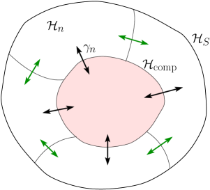
Figure 1: The Zeno subspaces are formed when the frequency $\tau^{-1}$ of measurements or BB pulses or the strength $K$ of the continuous coupling tend to $\infty$. The shaded region represents the “computational” subspace ${\cal H}_{\rm comp}\subset{\cal H}_{S}$ defined in Eq. (4). The transition rates $\gamma_{n}$ depend on $\tau$ or $K$.

III Master equation

We consider the time evolution when the initial state is factorized as in (5) and the reservoir equilibrium state has inverse temperature $\beta$

$$\rho_{B}={1\over Z}\exp(-\beta H_{B})={1\over Z}\sum_{\mu}\exp(-\beta E_{\mu})|\mu{\rangle}{\langle}\mu|,\qquad({\mathcal{L}}_{B}\rho_{B}=0)$$ (40)

where $Z=\mathrm{tr}_{B}e^{-\beta H_{B}}=\sum_{\mu}e^{-\beta E_{\mu}}$ is the normalization constant. We will assume throughout our analysis that the characteristic timescales of quantum state manipulation in the space ${\cal H}_{\rm comp}$ [see (4)] are much longer than any other timescales, so that the process is well described by the van Hove $``\lambda^{2}t"$ limit vanHove ; SpohnLeb ; AVL ; Yuasa , where $\lambda$ is the coupling constant between system and reservoir [see the comment after Eq. (3)]. For instance, if we take the timescale of quantum state manipulation to be of order $\lambda^{-2}$ ($\sim$ to a Rabi period in ${\cal H}_{\rm comp}$), then the other energies involved are at most O($\lambda^{0}$). We will look at some concrete examples in Sec. VII.

Following Gardiner and Zoller GardinerZoller , we now quickly derive the master equation and set up our notation. The starting point is the decomposition of the Liouville equation with the aid of the projection operators

$${\cal P}\rho=\mathrm{tr}_{B}\{\rho\}\otimes\rho_{B}=\sigma\otimes\rho_{B},\qquad{\mathcal{Q}}=1-{\mathcal{P}}$$ (41)

where ${\rm tr}_{B}$ stands for the partial trace over the reservoir degrees of freedom and $\rho_{B}$ is the equilibrium reservoir state (40). Note that ${\mathcal{P}}^{2}={\mathcal{P}}$ and ${\mathcal{Q}}^{2}={\mathcal{Q}}$. Moreover,

$${\mathcal{P}}{\mathcal{L}}_{S}={\mathcal{L}}_{S}{\mathcal{P}},\qquad{\mathcal{P}}{\mathcal{L}}_{B}={\mathcal{L}}_{B}{\mathcal{P}}=0$$ (42)

and we assume that

$${\mathcal{P}}{\mathcal{L}}_{SB}{\mathcal{P}}=0,$$ (43)

which can always be satisfied by redefining the system Liouville operator ${\mathcal{L}}_{S}\rho\to{\mathcal{L}}_{S}\rho+\mathrm{tr}_{B}\{{\mathcal{L}}_{SB}\rho\}\otimes\rho_{B}$ and the interaction Liouville operator ${\mathcal{L}}_{SB}\rho\to{\mathcal{L}}_{SB}\rho-\mathrm{tr}_{B}\{{\mathcal{L}}_{SB}\rho\}\otimes\rho_{B}$.

The evolution in the interaction picture reads

$$\dot{\rho}_{\mathrm{I}}(t)={\mathcal{L}}_{SB}(t)\rho_{\mathrm{I}}(t),\qquad{\mathcal{L}}_{SB}(t)=e^{-{\mathcal{L}}_{0}t}{\mathcal{L}}_{SB}e^{{\mathcal{L}}_{0}t}$$ (44)

and by applying the projection (41) together with Eq. (43) one gets

$${\mathcal{P}}\dot{\rho}_{\mathrm{I}}(t)={\mathcal{P}}{\mathcal{L}}_{SB}(t){\mathcal{Q}}\rho_{\mathrm{I}}(t),\qquad{\mathcal{Q}}\dot{\rho}_{\mathrm{I}}(t)={\mathcal{Q}}{\mathcal{L}}_{SB}(t){\mathcal{P}}\rho_{\mathrm{I}}(t)+{\mathcal{Q}}{\mathcal{L}}_{SB}(t){\mathcal{Q}}\rho_{\mathrm{I}}(t).$$ (45)

By formally integrating the second equation and plugging the result into the first one, one obtains to order $\lambda^{2}$

$${\mathcal{P}}\dot{\rho}_{\mathrm{I}}(t)=\int_{0}^{t}ds\;{\mathcal{P}}{\mathcal{L}}_{SB}(t){\mathcal{Q}}{\mathcal{L}}_{SB}(s){\mathcal{P}}\rho_{\mathrm{I}}(s),$$ (46)

where the initial condition (5), yielding ${\mathcal{Q}}\rho_{\mathrm{I}}(0)=0$, was used. By using the definitions (41) and the conditions (42)-(43), Eq. (46) yields

$$\dot{\sigma}_{\mathrm{I}}(t)=\int_{0}^{t}ds\,{\mathcal{K}}_{\mathrm{I}}(t,s)\sigma_{\mathrm{I}}(s),$$ (47)

where

$${\mathcal{K}}_{\mathrm{I}}(t,s)\,\sigma=\mathrm{tr}_{B}\left\{{\mathcal{L}}_{SB}(t){\mathcal{L}}_{SB}(s)\,\sigma\otimes\rho_{B}\right\}.$$ (48)

By making use of the first Markov approximation $\sigma_{\mathrm{I}}(s)\to\sigma_{\mathrm{I}}(t)$ GardinerZoller , which is motivated by the fact that the bath correlation kernel ${\mathcal{K}}_{\mathrm{I}}(t,s)$ is different from zero only for $s\simeq t-\tau_{c}$ such that $\sigma_{\mathrm{I}}(t-\tau_{c})\simeq\sigma_{\mathrm{I}}(t)$, one gets

$$\dot{\sigma}_{\mathrm{I}}(t)={\mathcal{L}}(t)\sigma_{\mathrm{I}}(t),\qquad{\mathcal{L}}(t)=\int_{0}^{t}ds\,{\mathcal{K}}_{\mathrm{I}}(t,s)\ .$$ (49)

If the time $t$ in Eqs. (49) is much larger than the bath correlation time, $t\gg\tau_{c}$, one can safely replace the upper limit of integration with $\infty$, getting a Markovian equation with the time independent Liouville operator ${\mathcal{L}}={\mathcal{L}}(\infty)$.

We emphasize that this procedure can be rigorously justified in the (weak coupling) limit AVL

$${\mathcal{L}}=\lim_{\lambda\to 0}\int_{0}^{t/\lambda^{2}}ds\,{\mathcal{K}}_{\mathrm{I}}(t/\lambda^{2},s),$$ (50)

which physically corresponds to a time coarse-graining ansatz Pauli ; LBW . From (48) and (50) one gets (by suppressing, for simplicity, the subscript I for the operators in the interaction picture)

$${\mathcal{L}}\,\sigma = \lim_{\lambda\to 0}\;\mathrm{tr}_{B}\left\{e^{-{\mathcal{L}}_{S}\,t/\lambda^{2}}\left[\int_{-t/\lambda^{2}}^{0}ds\;{\mathcal{L}}_{SB}{\mathcal{L}}_{SB}(s)\right]e^{{\mathcal{L}}_{S}\,t/\lambda^{2}}\,\sigma\otimes\rho_{B}\right\}$$ (51)

$$= \mathrm{tr}_{B}\left\{\sum_{\omega}\tilde{Q}_{\omega}\left[\int_{-\infty}^{0}ds\;{\mathcal{L}}_{SB}{\mathcal{L}}_{SB}(s)\right]\tilde{Q}_{\omega}\,\sigma\otimes\rho_{B}\right\},$$

where $\tilde{Q}_{\omega}$ are the eigenprojections of the Liouvillian ${\mathcal{L}}_{S}$,

$${\mathcal{L}}_{S}=-i\sum_{\omega}\omega\tilde{Q}_{\omega},\quad\sum_{\omega}\tilde{Q}_{\omega}=1,\quad\tilde{Q}_{\omega}\tilde{Q}_{\omega^{\prime}}=\delta_{\omega,\omega^{\prime}}\tilde{Q}_{\omega}\ ,$$ (52)

and in the limit the off-diagonal terms, $e^{i(\omega-\omega^{\prime})t/\lambda^{2}}\tilde{Q}_{\omega}[\cdots]\tilde{Q}_{\omega^{\prime}}$, vanish due to the Riemann-Lesbegue lemma. Notice that the superoperators $\tilde{Q}_{\omega}$ can be expressed in terms of the eigenprojections of the Hamiltonian $H_{S}$ as

$$\tilde{Q}_{\omega}\rho=\sum_{\scriptstyle m,n\atop\scriptstyle E_{m}-E_{n}=\omega}Q_{m}\rho Q_{n},\qquad H_{S}=\sum_{n}E_{n}Q_{n}\ .$$ (53)

From a physical point of view, the result (51) hinges upon a second-order perturbation expansion of the Liouvillian (3) in the interaction picture

$$e^{-{\mathcal{L}}_{0}t}e^{{\cal L}_{\rm tot}t}={\cal T}\exp\left(\int_{0}^{t}ds\;{\mathcal{L}}_{SB}(s)\right)\simeq\openone+\int_{0}^{t}ds\;{\mathcal{L}}_{SB}(s)+\int_{0}^{t}ds\int_{0}^{s}ds_{1}\;{\mathcal{L}}_{SB}(s){\mathcal{L}}_{SB}(s_{1}).$$ (54)

Indeed, the first-order term vanishes after the projection due to (43), while the projected second-order term reads

$$\mathrm{tr}_{B}\left\{\int_{0}^{t}ds\int_{0}^{s}ds_{1}\;{\mathcal{L}}_{SB}(s){\mathcal{L}}_{SB}(s_{1})\,\sigma\otimes\rho_{B}\right\}=\int_{0}^{t}ds\;\mathrm{tr}_{B}\left\{e^{-{\mathcal{L}}_{S}s}\left[\int_{-s}^{0}ds_{1}\;{\mathcal{L}}_{SB}{\mathcal{L}}_{SB}(s_{1})\right]e^{{\mathcal{L}}_{S}s}\,\sigma\otimes\rho_{B}\right\}$$

$$\simeq\int_{0}^{t}ds\;\mathrm{tr}_{B}\left\{e^{-{\mathcal{L}}_{S}s}\left[\int_{-\infty}^{0}ds_{1}\;{\mathcal{L}}_{SB}{\mathcal{L}}_{SB}(s_{1})\right]e^{{\mathcal{L}}_{S}s}\,\sigma\otimes\rho_{B}\right\}\simeq t\;\mathrm{tr}_{B}\left\{\sum_{\omega}\tilde{Q}_{\omega}\left[\int_{-\infty}^{0}ds\;{\mathcal{L}}_{SB}{\mathcal{L}}_{SB}(s)\right]\tilde{Q}_{\omega}\,\sigma\otimes\rho_{B}\right\}$$

$$={\mathcal{L}}t\;\sigma\ .$$ (55)

In the second equality we considered times $t$ much larger than the bath correlation time $\tau_{c}$, so that the integration range can be extended from $(-s,0)$ to $(-\infty,0)$, while in the third equality we neglected the rapidly oscillating (compared with those responsible for decoherence) off-diagonal terms. By combining (55) and (54) we finally get

$$\sigma_{\mathrm{I}}(t)=\mathrm{tr}_{B}\left\{e^{-{\mathcal{L}}_{0}t}e^{{\cal L}_{\rm tot}t}\,\sigma_{\mathrm{I}}(0)\otimes\rho_{B}\right\}\simeq\exp\left({\mathcal{L}}t\right)\sigma_{\mathrm{I}}(0)\ ,$$ (56)

which is nothing but (49), when one substitutes ${\mathcal{L}}(t)\to{\mathcal{L}}(\infty)={\mathcal{L}}$.

Some of these ideas and techniques, at different levels of rigor, have been investigated and applied in the literature of the last four decades vanHove ; SpohnLeb ; Yuasa .

III.1 The general case

Assume now that the interaction Hamiltonian $H_{SB}$ can be written as GardinerZoller

$$H_{SB}=\sum_{m}\left(X_{m}\otimes A^{\dagger}_{m}+X^{\dagger}_{m}\otimes A_{m}\right),$$ (57)

where the $X_{m}$ are the eigenoperators of the system Liouvillian, satisfying

$${\mathcal{L}}_{S}X_{m}=i\omega_{m}X_{m}\qquad(\omega_{m}\neq\omega_{n},\quad\mathrm{for}\quad m\neq n)$$ (58)

and $A_{m}$ are destruction operators of the bath

$$A_{m}=A(g_{m})=\int d^{3}k\;g_{m}^{*}(\bm{k})\;a(\bm{k})\ ,$$ (59)

expressed in terms of bosonic operators $a(\bm{k})$, with form factors $g_{m}(\bm{k})$. We are specifying our analysis to three dimensions (although it is valid in any dimensions). Incidentally, the form of the Hamiltonian (57) is of very general validity (and is not limited, as one might naively think, to dipole-like approximations): the only assumption made is that the coupling with the bath be linear, i.e. one is not considering terms of the type $a^{2},a^{\dagger 2}$, etc., which would only be relevant for squeezed reservoirs. In practice, one determines the operators (58), then finds the bath operators in order to write the interaction in the form (57), and neglects nonlinear terms.

In the interaction representation we get

$$H_{SB}(t)=e^{-{\mathcal{L}}_{0}t}H_{SB}=\sum_{m}\left(X_{m}\otimes A^{\dagger}_{m}(t)+X^{\dagger}_{m}\otimes A_{m}(t)\right),$$ (60)

where

$$A_{m}(t)=\int d^{3}k\;g_{m}^{*}(\bm{k})\;e^{-i(\omega_{k}-\omega_{m})t}a(\bm{k})\ .$$ (61)

If the bath is in the thermal state (40) we obtain

$$\left\langle A_{m}(t)A_{m}^{\dagger}(s)\right\rangle = \int d^{3}k\;|g_{m}(\bm{k})|^{2}\left(N(\omega_{k})+1\right)e^{-i(\omega_{k}-\omega_{m})(t-s)}\ ,$$

$$\left\langle A_{m}^{\dagger}(t)A_{m}(s)\right\rangle = \int d^{3}k\;|g_{m}(\bm{k})|^{2}N(\omega_{k})e^{i(\omega_{k}-\omega_{m})(t-s)}\,$$ (62)

and $\left\langle A_{m}(t)A_{m}(s)\right\rangle=\left\langle A_{m}^{\dagger}(t)A_{m}^{\dagger}(s)\right\rangle=0$, with $N(\omega)=1/(e^{\beta\omega}-1)$.

From (51) we get

$${\mathcal{L}}\sigma=\int_{-\infty}^{0}ds\;\mathrm{tr}_{B}\left\{\tilde{Q}_{\omega}{\mathcal{L}}_{SB}{\mathcal{L}}_{SB}(s)\tilde{Q}_{\omega}\sigma\otimes\rho_{B}\right\}$$ (63)

and by using the property

$$\sum_{\omega}\tilde{Q}_{\omega}{\mathcal{L}}_{1}{\mathcal{L}}_{2}\tilde{Q}_{\omega}\rho=-\sum_{\omega}\tilde{Q}_{\omega}\left[H_{1},\left[H_{2},\tilde{Q}_{\omega}\rho\right]\right]=-\sum_{\omega}\left[(\tilde{Q}_{\omega}H_{1}),\left[(\tilde{Q}_{-\omega}H_{2}),\rho\right]\right]\ ,$$ (64)

which easily follows from the definition (52), we get

$${\mathcal{L}}\sigma=-\sum_{\omega}\int_{-\infty}^{0}ds\;\mathrm{tr}_{B}\left\{\left[\left(\tilde{Q}_{\omega}H_{SB}\right),\left[\left(\tilde{Q}_{-\omega}H_{SB}(s)\right),\sigma\otimes\rho_{B}\right]\right]\right\}.$$ (65)

By using (53) and (57) one obtains

$$\tilde{Q}_{\omega_{m}}H_{SB}=H_{SB}^{(m)}=X_{-m}\otimes A^{\dagger}_{-m}+X^{\dagger}_{m}\otimes A_{m},$$ (66)

whence

$${\mathcal{L}}\sigma = -\sum_{m}\int_{-\infty}^{0}ds\;\mathrm{tr}_{B}\left\{\left[H_{SB}^{(m)},\left[H_{SB}^{(-m)}(s),\sigma\otimes\rho_{B}\right]\right]\right\}$$ (67)

$$= -\sum_{m}\int_{-\infty}^{0}ds\;\mathrm{tr}_{B}\left\{\left[X^{\dagger}_{m}\otimes A_{m},\left[X_{m}\otimes A^{\dagger}_{m}(s),\sigma\otimes\rho_{B}\right]\right]+\left[X_{-m}\otimes A^{\dagger}_{-m},\left[X^{\dagger}_{-m}\otimes A_{-m}(s),\sigma\otimes\rho_{B}\right]\right]\right\}\ .\$$

In the second equality we neglected terms containing two annihilation or creation operators, which identically vanish by performing the trace over the thermal state $\rho_{B}$. Equation (67) can be put in the form GardinerZoller

$${\mathcal{L}}\sigma = -i\sum_{m}\left[\delta_{m}X_{m}^{\dagger}X_{m}+\epsilon_{m}X_{m}X_{m}^{\dagger},\sigma\right]$$ (68)

$$+\sum_{m}K_{m}\left(X_{m}\sigma X_{m}^{\dagger}-\frac{1}{2}\left\{X_{m}^{\dagger}X_{m},\sigma\right\}\right)+\sum_{m}G_{m}\left(X_{m}^{\dagger}\sigma X_{m}-\frac{1}{2}\left\{X_{m}X_{m}^{\dagger},\sigma\right\}\right)\ ,$$

and

$$\frac{1}{2}K_{m}-i\delta_{m}=\int_{0}^{\infty}dt\left\langle A_{m}(0)A_{m}^{\dagger}(t)\right\rangle\ ,\qquad\frac{1}{2}G_{m}-i\epsilon_{m}=\int_{0}^{\infty}dt\left\langle A_{m}^{\dagger}(0)A_{m}(t)\right\rangle\ .$$ (69)

The first line in (68) is just the renormalization of the free Liouvillian ${\mathcal{L}}_{S}$ by Lamb and Stark shift terms and will be neglected in the following. The dissipative part is given by the second line, which appears in the Lindblad form, so that $\mathrm{tr{\mathcal{L}}\sigma}=0$.

In Eq. (58) we will identify $\omega_{-m}=-\omega_{m}$, and will assume that $X_{-m}=X_{m}^{\dagger}$ and $g_{m}=g_{-m}$, which is equivalent to the hypothesis that the interaction Hamiltonian be the product of selfadjoint operators acting on the system and the bath, namely $H_{SB}=\sum_{i}H_{S}^{(i)}\otimes H_{B}^{(i)}$, with $H_{S}^{(i)}$ and $H_{B}^{(i)}$ selfadjoint. Notice, therefore, that we are not making any rotating-wave approximation, and the interaction Hamiltonian $H_{SB}$ (57) contains both rotating and counter-rotating terms. The dissipative part of (68) can now be rewritten as

$${\mathcal{L}}\sigma = \gamma_{0}\left(X_{0}\sigma X_{0}-\frac{1}{2}\left\{X_{0}X_{0},\sigma\right\}\right)$$ (70)

$$+\sum_{m\geq 1}\gamma_{m}\left(X_{m}\sigma X_{m}^{\dagger}-\frac{1}{2}\left\{X_{m}^{\dagger}X_{m},\sigma\right\}\right)+\sum_{m\geq 1}\gamma_{-m}\left(X_{m}^{\dagger}\sigma X_{m}-\frac{1}{2}\left\{X_{m}X_{m}^{\dagger},\sigma\right\}\right)\ ,$$

where $\gamma_{m}=K_{m}+G_{-m}$. We introduce the bare spectral density functions (form factors)

$$\kappa_{m}(\omega)=\int d^{3}k\;|g_{m}(\bm{k})|^{2}\delta(\omega_{k}-\omega),\qquad\kappa_{m}(\omega)=0,\quad\mathrm{for}\quad\omega<0$$ (71)

and the thermal spectral density functions,

$$\kappa_{m}^{\beta}(\omega)=\kappa_{m}(\omega)\left(N(\omega)+1\right)+\kappa_{m}(-\omega)N(-\omega)=\frac{1}{1-e^{-\beta\omega}}\left[\kappa_{m}(\omega)-\kappa_{m}(-\omega)\right],$$ (72)

which extend along the whole real axis due to the counter-rotating terms and satisfy the KMS symmetry SpohnLeb

$$\kappa_{m}^{\beta}(-\omega)=\frac{N(\omega)}{N(\omega)+1}\,\kappa_{m}^{\beta}(\omega)=\frac{N(-\omega)+1}{N(-\omega)}\,\kappa_{m}^{\beta}(\omega)=\exp(-\beta\omega)\,\kappa_{m}^{\beta}(\omega).$$ (73)

We explicitly get

$$K_{m}=2\pi\kappa_{m}(\omega_{m})\,\left(N(\omega_{m})+1\right),\qquad G_{m}=2\pi\kappa_{m}(\omega_{m})\,N(\omega_{m})$$ (74)

and

$$\gamma_{m}=2\mathrm{\,Re}\int_{0}^{\infty}dt\left(\left\langle A_{m}A^{\dagger}_{m}(t)\right\rangle+\left\langle A_{-m}^{\dagger}A_{-m}(t)\right\rangle\right)=2\pi\kappa_{m}^{\beta}(\omega_{m})\ .$$ (75)

It is useful to look at some concrete examples and scrutinize the modification of the form factor (71), due to the presence of the thermal bath. Let us focus, for the sake of clarity, on two particular Ohmic cases: an exponential form factor

$$\kappa_{m}^{(E)}(\omega)=g^{2}\omega\exp(-\omega/\Lambda)\theta(\omega)$$ (76)

and a polynomial form factor

$$\kappa^{(P)}_{m}(\omega)=g^{2}\frac{\omega}{[1+(\omega/\Lambda)^{2}]^{n}}\theta(\omega).$$ (77)

In the latter case, we focus on $n=2$, which is typical of quantum dots qdot (the case $n=4$ is also of interest, being the nonrelativistic form factor of the 2P-1S transition of the hydrogen atom Hff ; PLA98 ). In the above formulas, $g$ is a coupling constant, $\Lambda$ a cutoff and $\theta$ the unit step function.

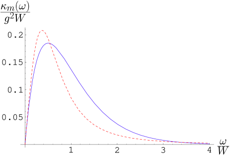
Figure 2: The form factors at zero temperature, $\kappa(\omega)/(g^{2}W)$ vs $\omega/W$. Full line: exponential form factor (76); dashed line: polynomial form factor (77).

In order to properly compare these two cases, we will require that the bandwidth be the same:

$$W={\int_{-\infty}^{\infty}d\omega\;|\omega|\kappa^{(E)}_{m}(\omega)\over\int_{-\infty}^{\infty}d\omega\;\kappa^{(E)}_{m}(\omega)}={\int_{-\infty}^{\infty}d\omega\;|\omega|\kappa^{(P)}_{m}(\omega)\over\int_{-\infty}^{\infty}d\omega\;\kappa^{(P)}_{m}(\omega)},$$ (78)

where the square root of the denominator

$$\left[\int_{-\infty}^{\infty}d\omega\;\kappa_{m}(\omega)\right]^{-{1\over 2}}\equiv\tau_{\mathrm{Z}}$$ (79)

is the so-called Zeno time, characterizing the convexity of the survival probability at the origin PLA98 ; Antoniou ; PIO . Notice that a finite natural cutoff $\Lambda\simeq 8.498\cdot 10^{18}\mbox{rad/s}$ and a finite Zeno time $\tau_{\rm Z}\simeq 3.593\cdot 10^{-15}\mbox{s}$ can also be computed for the hydrogen atom in vacuum [polynomial form factor (77) with $n=4$], as well as for atomic and molecular systems whose electronic wave functions are known. The condition (78) when $n=2$ yields the ratio $\Lambda_{\rm pol}/\Lambda_{\rm exp}=1.275$ between the cutoffs for the polynomial and exponential form factors, and $W=1.99\Lambda_{\rm exp}$. The two form factors are displayed in Fig. 2 for $g=1$.

The thermal form factors (72) are displayed in Fig. 3 for two different temperatures. Three features are apparent: the form factor is an increasing function of the temperature $\beta^{-1}$. Its value at $\omega=0$ is $\kappa_{m}^{\beta}(0)=\kappa^{\prime}_{m}(0^{+})/\beta=g^{2}/\beta$, where the prime denotes derivative. Moreover, its derivative reads $\kappa_{m}^{\beta\prime}(0^{\pm})=\kappa^{\prime}_{m}(0^{+})/2\pm\kappa^{\prime\prime}_{m}(0^{+})/(2\beta)$, whence it is continuous, $\kappa_{m}^{\beta\prime}(0)=g^{2}/2$, in the polynomial case (because $\kappa^{\prime\prime}_{m}(0^{+})=0$), and discontinuous, $\kappa_{m}^{\beta\prime}(0^{\pm})=g^{2}/2\mp g^{2}/(\beta\Lambda)$, in the exponential case; this is more apparent at higher temperatures. Finally, the support of the thermal form factors is no longer lower bounded, due to the effect of the counter-rotating terms.

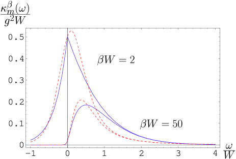
Figure 3: The thermal form factors $\kappa_{m}^{\beta}(\omega)$ vs $\omega$. Full lines: exponential form factors (72), (76); dashed lines: polynomial form factors (72), (77). The form factor is larger at higher temperature $\beta^{-1}$. Note the discontinuity of the derivative in the exponential case at $\omega=0$ (more apparent at high temperature). We set $\beta W=50$ (low temperature) and $\beta W=2$ (very high temperature).

III.2 Two-level system

A particular case of the above is the qubit Hamiltonian

$$H_{0}=\frac{\Omega}{2}\sigma_{z},\qquad H_{SB}=\sigma_{z}\otimes\left(A(g_{0})+A^{\dagger}(g_{0})\right)+\sigma_{x}\otimes\left(A(g_{1})+A^{\dagger}(g_{1})\right).$$ (80)

This is of the form (57), when one identifies

$$X_{0}=\sigma_{z},\quad X_{\pm 1}=\sigma_{\mp}=\frac{\sigma_{x}\mp i\sigma_{y}}{2},\quad\omega_{\pm 1}=\pm\Omega,\quad\omega_{0}=0,$$ (81)

hence

$${\mathcal{L}}\rho=\gamma_{0}\left(\sigma_{z}\rho\sigma_{z}-\rho\right)+\gamma_{+1}\left(\sigma_{-}\rho\sigma_{+}-\frac{1}{2}\left\{\sigma_{+}\sigma_{-},\rho\right\}\right)+\gamma_{-1}\left(\sigma_{+}\rho\sigma_{-}-\frac{1}{2}\left\{\sigma_{-}\sigma_{+},\rho\right\}\right)\ ,$$ (82)

with

$$\gamma_{0}=2\pi\kappa_{0}^{\beta}(0)=2\pi\frac{\kappa^{\prime}_{0}(0^{+})}{\beta},\qquad\gamma_{\pm 1}=2\pi\kappa_{1}^{\beta}(\pm\Omega)\ ,$$ (83)

where we used (72).

IV Quantum Zeno Control

Let us look at the quantum Zeno dynamics with a finite interval $\tau=t/N$ between measurements,

$$\rho(t)=\left[{\hat{P}}e^{{\cal L}_{\rm tot}\tau}{\hat{P}}\right]^{\frac{t}{\tau}}\rho(0)\ ,$$ (84)

where ${\mathcal{L}}_{\mathrm{tot}}$ and ${\hat{P}}$ are given by (3) and (7), respectively. We will look at the subtle effects on the decay rate arising from the presence of the short-time quadratic (Zeno) region. Therefore the standard method vanHove is not applicable to the present situation and the limit must be evaluated by a different technique. We only sketch the main steps in the derivation and give more details in Appendix B. Second order perturbation in ${\mathcal{L}}_{SB}$ and the conditions (8)-(9) yield

$${\hat{P}}e^{{\cal L}_{\rm tot}\tau}{\hat{P}}={\hat{P}}e^{{\mathcal{L}}_{0}\tau}{\cal T}\exp\left(\int_{0}^{\tau}ds\;{\mathcal{L}}_{SB}(s)\right){\hat{P}}\simeq e^{{\mathcal{L}}_{0}\tau}{\hat{P}}\left[\openone+\int_{0}^{\tau}ds\;{\mathcal{L}}_{SB}(s)+\int_{0}^{\tau}ds\int_{0}^{s}ds_{1}\;{\mathcal{L}}_{SB}(s){\mathcal{L}}_{SB}(s_{1})\right]{\hat{P}}\ .$$ (85)

In terms of the operator ${\mathcal{G}}_{\mathrm{Z}}(\tau)$, defined as the solution of the operator equation

$$\int_{0}^{\tau}ds\;e^{-{\mathcal{L}}_{0}s}{\mathcal{G}}_{\mathrm{Z}}(\tau)e^{{\mathcal{L}}_{0}s}={\hat{P}}\int_{0}^{\tau}ds\int_{0}^{s}ds_{1}\;{\mathcal{L}}_{SB}(s){\mathcal{L}}_{SB}(s_{1}){\hat{P}}=\int_{0}^{\tau}ds\;e^{-{\mathcal{L}}_{0}s}\left[\int_{0}^{s}ds_{1}\;{\hat{P}}{\mathcal{L}}_{SB}{\mathcal{L}}_{SB}(-s_{1}){\hat{P}}\right]e^{{\mathcal{L}}_{0}s}\ ,$$ (86)

one obtains

$$\left[{\hat{P}}e^{{\mathcal{L}}_{\rm tot}\tau}{\hat{P}}\right]^{t/\tau}\simeq\left[{\hat{P}}e^{{\mathcal{L}}_{0}\tau}{\cal T}\exp\left(\int_{0}^{\tau}ds\;e^{-{\mathcal{L}}_{0}s}{\mathcal{G}}_{\mathrm{Z}}(\tau)e^{{\mathcal{L}}_{0}s}\right){\hat{P}}\right]^{t/\tau}={\hat{P}}\exp\left\{[{\mathcal{L}}_{0}+{\mathcal{G}}_{\mathrm{Z}}(\tau)]t\right\}.$$ (87)

Under the assumption that the bath state can well be approximated by an equilibrium state at time $t$, the final reduced state $\sigma(t)$ is shown to satisfy the equation

$$\dot{\sigma}(t)=\left[{\mathcal{L}}_{S}+{\mathcal{L}}_{\mathrm{Z}}(\tau)\right]\sigma(t)\ ,$$ (88)

with

$${\mathcal{L}}_{\mathrm{Z}}(\tau)\sigma=\mathrm{tr}_{B}\left\{{\mathcal{G}}_{\mathrm{Z}}(\tau)\sigma\otimes\rho_{B}\right\}\ .$$ (89)

Note that ${\mathcal{L}}_{\mathrm{Z}}(\tau)$ is the solution of the operator equation

$$\int_{0}^{\tau}dt\;e^{-{\mathcal{L}}_{S}t}{\mathcal{L}}_{\mathrm{Z}}(\tau)e^{{\mathcal{L}}_{S}t}=\int_{0}^{\tau}dt{\hat{P}}{\mathcal{L}}(t){\hat{P}}=\int_{0}^{\tau}dt\int_{0}^{t}ds\;{\hat{P}}{\mathcal{K}}_{\mathrm{I}}(t,s){\hat{P}}\ .$$ (90)

where ${\mathcal{K}}_{\mathrm{I}}$ is defined in (48). The dissipative part of (89) is found to have the explicit form [analogous to Eq. (70)]

$${\mathcal{L}}_{\mathrm{Z}}(\tau)\sigma = \gamma_{0}^{\mathrm{Z}}(\tau){\hat{P}}\left(X_{0}{\hat{P}}\sigma X_{0}-\frac{1}{2}\left\{X_{0}X_{0},{\hat{P}}\sigma\right\}\right)$$

$$+\sum_{m\geq 1}\gamma_{m}^{\mathrm{Z}}(\tau){\hat{P}}\left(X_{m}{\hat{P}}\sigma X_{m}^{\dagger}-\frac{1}{2}\left\{X_{m}^{\dagger}X_{m},{\hat{P}}\sigma\right\}\right)+\sum_{m\geq 1}\gamma_{-m}^{\mathrm{Z}}(\tau){\hat{P}}\left(X_{m}^{\dagger}{\hat{P}}\sigma X_{m}-\frac{1}{2}\left\{X_{m}X_{m}^{\dagger},{\hat{P}}\sigma\right\}\right)\ ,$$

where the controlled decay rates read

$$\gamma_{m}^{\mathrm{Z}}(\tau)=\frac{2}{\tau}\mathrm{\,Re}\int_{0}^{\tau}dt\int_{-t}^{0}ds\left(\left\langle A_{m}A^{\dagger}_{m}(s)\right\rangle+\left\langle A_{-m}^{\dagger}A_{-m}(s)\right\rangle\right)=\tau\int_{-\infty}^{\infty}d\omega\;\kappa_{m}^{\beta}(\omega)\;{\rm sinc}^{2}\left(\frac{\omega-\omega_{m}}{2}\tau\right)\ ,$$ (92)

with $\mathrm{sinc}(x)=\sin(x)/x$. This yields Zeno and inverse Zeno effects as $\tau$ is changed, as we will see in Sec. VII. The key issue, once again, is to understand how small $\tau$ should be in order to get suppression (control) of decoherence (QZE), rather than its enhancement (IZE).

V Control via dynamical decoupling

We can now investigate the nonideal bang-bang control of decoherence. From Eq. (29), describing a BB control with a single kick bang ,

$$\rho(t)=\left[e^{{\mathcal{L}}_{\mathrm{k}}}e^{{\cal L}_{\rm tot}\tau}\right]^{\frac{t}{\tau}}\rho(0)\ ,$$ (93)

where ${\mathcal{L}}_{\mathrm{tot}}$ is again given by (3). As in the Zeno control, we consider here the case where $\tau$ is finite, so that the effects on the decay rate arising from the presence of a short-time quadratic (Zeno) region play a fundamental role. Once again, we only sketch the main steps in the derivation and give more details in Appendix C. Second order perturbation in ${\mathcal{L}}_{SB}$ yields

$$e^{{\mathcal{L}}_{\mathrm{k}}}e^{{\cal L}_{\rm tot}\tau}=e^{{\mathcal{L}}_{\mathrm{k}}}e^{{\mathcal{L}}_{0}\tau}{\cal T}\exp\left(\int_{0}^{\tau}ds\;{\mathcal{L}}_{SB}(s)\right)\simeq e^{{\mathcal{L}}_{\mathrm{k}}}e^{{\mathcal{L}}_{0}\tau}\left[\openone+\int_{0}^{\tau}ds\;{\mathcal{L}}_{SB}(s)+\int_{0}^{\tau}ds\int_{0}^{s}ds_{1}\;{\mathcal{L}}_{SB}(s){\mathcal{L}}_{SB}(s_{1})\right]\ .$$ (94)

In terms of the operators ${\mathcal{F}}_{\mathrm{k}}(\tau)$ and ${\mathcal{G}}_{\mathrm{k}}(\tau)$, defined as solutions of the operator equations

$$\int_{0}^{\tau}ds\;e^{-{\mathcal{L}}_{\tau}s}{\mathcal{F}}_{\mathrm{k}}(\tau)e^{{\mathcal{L}}_{\tau}s}=\int_{0}^{\tau}ds\;{\mathcal{L}}_{SB}(s)$$ (95)

$$\int_{0}^{\tau}ds\;e^{-{\mathcal{L}}_{\tau}s}{\mathcal{G}}_{\mathrm{k}}(\tau)e^{{\mathcal{L}}_{\tau}s}=\int_{0}^{\tau}ds\int_{0}^{s}ds_{1}\;\left[{\mathcal{L}}_{SB}(s){\mathcal{L}}_{SB}(s_{1})-e^{-{\mathcal{L}}_{\tau}s}{\mathcal{F}}_{\mathrm{k}}(\tau)e^{{\mathcal{L}}_{\tau}(s-s_{1})}{\mathcal{F}}_{\mathrm{k}}(\tau)e^{{\mathcal{L}}_{\tau}s_{1}}\right]\ ,$$ (96)

with

$${\mathcal{L}}_{\tau}=\frac{{\mathcal{L}}_{\mathrm{k}}}{\tau}+{\mathcal{L}}_{0},$$ (97)

one has

$$\left[e^{{\mathcal{L}}_{\mathrm{k}}}e^{{\cal L}_{\rm tot}\tau}\right]^{N}\simeq\left[e^{{\mathcal{L}}_{\tau}\tau}{\cal T}\exp\left(\int_{0}^{\tau}ds\;e^{-{\mathcal{L}}_{\tau}s}\left({\mathcal{F}}_{\mathrm{k}}(\tau)+{\mathcal{G}}_{\mathrm{k}}(\tau)\right)e^{{\mathcal{L}}_{\tau}s}\right)\right]^{N}=\exp\left\{\left[\frac{{\mathcal{L}}_{\mathrm{k}}}{\tau}+{\mathcal{L}}_{0}+{\mathcal{F}}_{\mathrm{k}}(\tau)+{\mathcal{G}}_{\mathrm{k}}(\tau)\right]t\right\}.$$ (98)

With the aid of (98), the final reduced state $\sigma(t)$ satisfies the equation

$$\dot{\sigma}(t)=\left[\frac{{\mathcal{L}}_{k}}{\tau}+{\mathcal{L}}_{S}+{\mathcal{L}}_{\mathrm{k}}(\tau)\right]\sigma(t)\ ,$$ (99)

with

$${\mathcal{L}}_{\mathrm{k}}(\tau)\sigma=\mathrm{tr}_{B}\left\{{\mathcal{G}}_{\mathrm{k}}(\tau)\sigma\otimes\rho_{B}\right\}\ .$$ (100)

The dissipative part of (100) has the explicit form

$${\mathcal{L}}_{\mathrm{k}}(\tau)\sigma = \gamma_{0}^{\mathrm{k}}(\tau)\left(X_{0}(\tau)\sigma X_{0}(\tau)-\frac{1}{2}\left\{X_{0}(\tau)X_{0}(\tau),\sigma\right\}\right)+\sum_{m\geq 1}\gamma_{m}^{\mathrm{k}}(\tau)\left(X_{m}(\tau)\sigma X_{m}^{\dagger}(\tau)-\frac{1}{2}\left\{X_{m}^{\dagger}(\tau)X_{m}(\tau),\sigma\right\}\right)$$ (101)

$$+\sum_{m\geq 1}\gamma_{-m}^{\mathrm{k}}(\tau)\left(X_{m}^{\dagger}(\tau)\sigma X_{m}(\tau)-\frac{1}{2}\left\{X_{m}(\tau)X_{m}^{\dagger}(\tau)\sigma\right\}\right)\ ,$$

where, in analogy with Eq. (58), the $X_{m}(\tau)$ are the eigenoperators of the Liouvillian ${\mathcal{L}}_{\mathrm{k}}/\tau+{\mathcal{L}}_{S}$, satisfying

$$\left(\frac{{\mathcal{L}}_{\mathrm{k}}}{\tau}+{\mathcal{L}}_{S}\right)X_{m}(\tau)=i\omega_{m}(\tau)X_{m}(\tau)\qquad(\omega_{m}\neq\omega_{n},\quad\mathrm{for}\quad m\neq n)$$ (102)

and the controlled decay rates read

$$\gamma_{m}^{\mathrm{k}}(\tau)=2\mathrm{\,Re}\int_{0}^{\infty}dt\left(\left\langle\tilde{A}_{m}(0)\tilde{A}^{\dagger}_{m}(t)\right\rangle+\left\langle\tilde{A}_{-m}^{\dagger}(0)\tilde{A}_{-m}(t)\right\rangle\right)=2\pi\kappa_{m}^{\beta}\left(\omega_{m}(\tau)\right)=2\pi\kappa_{m}^{\beta}\left(\frac{2\pi m}{\tau}+\mathrm{O}(1)\right)\ ,$$ (103)

with

$$\tilde{A}_{m}(t)=\int d^{3}kg_{m}^{*}({\bm{k}})e^{-i(\omega_{k}-\omega_{m}(\tau))t}a({\bm{k}}).$$ (104)

Notice that the mechanism of decoherence suppression (103) is not fully determined by ${\mathcal{L}}_{\rm tot}$ and $\hat{P}$, in contrast to the Zeno case, and depends also on the details of the Liovillian ${\mathcal{L}}_{\mathrm{k}}$ through $\omega_{m}(\tau)$. This is best clarified by explicitly looking at a particular case: let us consider the two level system (80) with $g_{0}=0$ (spin-flip decoherence). We include an additional third level—that performs the control—and add to (80) the Hamiltonian (acting on $\mathcal{H}_{S}\oplus\mathrm{span}\{|M\rangle\}$)

$$H_{M}=-\frac{\Omega}{2}|M\rangle\langle M|,$$ (105)

so that $|M\rangle$ is degenerate with $|{\downarrow}\rangle$. The control consists of a sequence of $2\pi$ pulses ShiokawaLidar between $|{\downarrow}\rangle$ and $|M\rangle$, given by

$$U_{\mathrm{k}}=\exp\left[-i\pi\left(|{\downarrow}\rangle\langle M|+|M\rangle\langle{\downarrow}|\right)\right]=P_{\uparrow}-P_{-1}\;,$$ (106)

where

$$P_{\uparrow}=|\uparrow\rangle\langle\uparrow|,\qquad P_{-1}=P_{\downarrow}+P_{M}=|\downarrow\rangle\langle\downarrow|+|M\rangle\langle M|,$$ (107)

are the eigenprojections of $U_{\mathrm{k}}$ (belonging respectively to $e^{-i\lambda_{\uparrow}}=1$ and $e^{-i\lambda_{-1}}=-1$) which define two Zeno subspaces. In the $\tau\to 0$ limit any decoherence between these two subspaces is suppressed. In fact, the total decay rate of the upper level has been explicitly computed BBDDsem ; ShiokawaLidar and reads

$$\gamma_{\uparrow}^{\mathrm{k}}(\tau)=\lim_{t\to\infty}t\int_{-\infty}^{\infty}d\omega\;\kappa^{\beta}(\omega)\;{\rm sinc}^{2}\left(\frac{\omega-\Omega}{2}\,t\right)\tan^{2}\left(\frac{\omega-\Omega}{2}\,\tau\right)\ .$$ (108)

As a matter of fact, the function multiplying the thermal form factor inside the integral can be shown to have the interesting limit

$$\lim_{t\to\infty}t\;{\rm sinc}^{2}\left(\frac{\omega t}{2}\right)\tan^{2}\left(\frac{\omega\tau}{2}\right)=\frac{2}{\pi}\sum_{j=0}^{\infty}\frac{1}{\left(j+\frac{1}{2}\right)^{2}}\left[\delta\left(\omega-\frac{2\pi}{\tau}(j+1/2)\right)+\delta\left(\omega+\frac{2\pi}{\tau}(j+1/2)\right)\right]\ .$$ (109)

The above limit is taken by keeping $\tau$ fixed—finite and nonvanishing—and $t=N\tau$, with $N$ integer and even ShiokawaLidar . By plugging (109) into (108) one gets

$$\gamma^{\mathrm{k}}_{\uparrow}(\tau)=\frac{2}{\pi}\sum_{j=0}^{\infty}\frac{1}{\left(j+\frac{1}{2}\right)^{2}}\left[\kappa^{\beta}\left(\Omega+\frac{2\pi}{\tau}(j+1/2)\right)+\kappa^{\beta}\left(\Omega-\frac{2\pi}{\tau}(j+1/2)\right)\right]\ ,$$ (110)

which is a sum of suitably weighted terms of the form (103). This yields again control of decoherence as $\tau$ is varied, as we will see in Sec. VII. The key issue, once again, is to understand how small $\tau$ should be in order to get suppression of decoherence (control), rather than its enhancement. Equation (110) yields also a significant computational advantage, when compared to (108): for well-behaved form factors (without resonances) the first few terms already provide a good estimate of the controlled lifetime.

VI Control via a strong continuous coupling

We can now analyze the last case, that of control by means of a strong continuous coupling. Since the control of decoherence is achieved by adding a control Hamiltonian $KH_{\mathrm{c}}$ acting on the Hilbert space $\mathcal{H}_{S}$, we begin with the study of the spectral properties of the new “system” Hamiltonian $H_{S}(K)\equiv H_{S}+KH_{\mathrm{c}}$. By writing the spectral resolutions of $H_{S}$ and $H_{\mathrm{c}}$,

$$H_{S}=\sum_{n}E_{n}Q_{n},\qquad H_{\mathrm{c}}=\sum_{m}\eta_{m}P_{m},$$ (111)

with $\sum_{n}Q_{n}=\sum_{m}P_{m}=\openone$, and by using the property (16) we see that $P_{mn}=P_{m}Q_{n}$ is a (finer) orthogonal resolution of the identity, i.e. $\sum_{m,n}P_{mn}=\openone$, with $P_{mn}P_{m^{\prime}n^{\prime}}=\delta_{m,m^{\prime}}\delta_{n,n^{\prime}}P_{mn}$. Note that some $P_{mn}$ can vanish. In particular $H^{\prime}_{S}$ can be explicitly diagonalized

$$H_{S}(K)=\sum_{m,n}\left(K\eta_{m}+E_{n}\right)P_{mn},\qquad P_{mn}=P_{m}Q_{n}\ .$$ (112)

Equations (111) and (112) directly translate in terms of Liouvillian as

$${\mathcal{L}}_{S}=-i\sum_{n}\omega_{n}{\tilde{Q}}_{n},\qquad{\mathcal{L}}_{\mathrm{c}}=-i\sum_{m}\Omega_{m}{\tilde{P}}_{m}$$ (113)

and

$${\mathcal{L}}_{S}(K) = {\mathcal{L}}_{S}+K{\mathcal{L}}_{\mathrm{c}}=-i\sum_{m,n}\omega_{mn}(K){\tilde{P}}_{mn},$$

$$\omega_{mn}(K) = K\Omega_{m}+\omega_{n},\qquad{\tilde{P}}_{mn}={\tilde{P}}_{m}{\tilde{Q}}_{n}\ .$$ (114)

The condition (8) for a complete control of decoherence, ${\hat{P}}H_{SB}=0$, leads to

$$0={\hat{P}}H_{SB}=\sum_{m}P_{m}H_{SB}P_{m}=\tilde{P}_{0}H_{SB}=\sum_{n}\tilde{P}_{0}\tilde{Q}_{n}H_{SB}=\sum_{n}\tilde{P}_{0n}H_{SB},$$ (115)

whence

$$\tilde{P}_{0n}H_{SB}=0,\qquad\forall n\ .$$ (116)

Therefore, by following exactly the same steps of Sec. III.1, with $H_{S}(K)$ defined by (112) in place of $H_{S}$, one obtains that the dissipative part of the Liouvillian ${\mathcal{L}}_{K}$ governing the slow evolution of the reduced density matrix $\sigma$ is given by

$${\mathcal{L}}_{K}\sigma = \sum_{m\geq 1,\,n}\gamma_{mn}(K)\left(X_{mn}\sigma X_{mn}^{\dagger}-\frac{1}{2}\left\{X_{mn}^{\dagger}X_{mn},\sigma\right\}\right)$$ (117)

$$+\sum_{m\geq 1,\,n}\gamma_{-m,n}(K)\left(X_{mn}^{\dagger}\sigma X_{mn}-\frac{1}{2}\left\{X_{mn}X_{mn}^{\dagger},\sigma\right\}\right)\ ,$$

where

$$X_{mn}\equiv\tilde{P}_{m}X_{n}\ ,$$ (118)

with $X_{n}$ given by (57)-(58), and

$$\gamma_{mn}(K)=2\mathrm{\,Re}\int_{0}^{\infty}dt\left(\left\langle\tilde{A}_{mn}(0)\tilde{A}^{\dagger}_{mn}(t)\right\rangle+\left\langle\tilde{A}_{-m,n}^{\dagger}(0)\tilde{A}_{-m,n}(t)\right\rangle\right)=2\pi\kappa_{n}^{\beta}\left(\omega_{mn}(K)\right)\ ,$$ (119)

with

$$\tilde{A}_{mn}(t)=\int d^{3}k\;g_{n}^{*}({\bm{k}})e^{-i(\omega_{k}-\omega_{mn}(K))t}a({\bm{k}})\ .$$ (120)

All terms with $m=0$ identically vanish due to (116). In the $K\to\infty$ limit, because the thermal form factor $\kappa_{m}^{\beta}(\omega)$ vanishes as $\omega\to\infty$ (cf. Fig. 2), one has

$$\gamma_{mn}(K)=2\pi\kappa_{n}^{\beta}\left(K\Omega_{m}+\omega_{n}\right)\sim 2\pi\kappa_{n}^{\beta}\left(K\Omega_{m}\right)\to 0\ ,\qquad\mbox{for}\quad K\to\infty\ .$$ (121)

Hence, in the $K\to+\infty$ limit, the dissipative part disappears, ${\mathcal{L}}_{K}\to 0$, or decoherence is suppressed, as expected.

It is interesting to observe that, when the condition (16) is not satisfied, the control via a strong continuous coupling needs an additional argument. In such a case, the control Hamiltonian $H_{c}$ and the system Hamiltonian $H_{S}$ cannot be simultaneously diagonalized, but (for a finite-dimensional ${\cal H}_{S}$), as a result of the analyticity of the eigenvalues and the corresponding eigenprojections of the Hermitian operator $H_{S}(K)/K=H_{S}/K+H_{c}$ with respect to the perturbation parameter $1/K$ KatoLinearOperators , the eigenvalues $\omega_{mn}(K)$ of the new system Liouvillian ${\cal L}_{S}(K)=K{\cal L}_{c}+{\cal L}_{S}$ and the corresponding eigenprojections ${\tilde{P}}_{mn}(K)$ satisfy

$$\omega_{mn}(K) = K\Omega_{m}+\Omega_{mn}^{(1)}+{\rm O}\left({1\over K}\right)\ ,$$ (122)

$${\tilde{P}}_{mn}(K) = {\tilde{P}}_{mn}^{(0)}+{1\over K}{\tilde{P}}_{mn}^{(1)}+{\rm O}\left({1\over K^{2}}\right)\ ,$$ (123)

where $\Omega_{mn}^{(1)}$ and ${\tilde{P}}_{mn}^{(j)}$ ($j=0,1$) do not depend on $K$. As in (116), one gets that ${\tilde{P}}_{0n}^{(0)}H_{SB}=0$, but this does not imply that ${\tilde{P}}_{0n}(K)H_{SB}=0$. As a result, there appear dissipative terms which tend to 0 via a different mechanism from the one outlined above. This aspect will be discussed elsewhere, together with similar phenomena that occur also for the other two control mechanisms (BB and Zeno).

In general, as in the BB control but in contrast to the Zeno case, the mechanism of decoherence suppression (121) is not fully determined by $H_{S}$ and depends on the details of the Hamiltonians $H_{S}$ and $H_{\mathrm{c}}$. Once again, this can be clarified by looking at a specific example: consider the two level system (80) with $g_{0}=0$ (spin flip decoherence). We add to (80) the Hamiltonian (acting on $\mathcal{H}_{S}\oplus\mathrm{span}\{|M\rangle\}$)

$$H_{M} = -\frac{\Omega}{2}|M\rangle\langle M|+KH_{\mathrm{c}},$$

$$H_{\mathrm{c}} = |{\downarrow}\rangle\langle M|+|M\rangle\langle{\downarrow}|=P_{+}-P_{-}\;,$$ (124)

where

$$P_{\pm}=\frac{(|{\downarrow}\rangle\pm|M\rangle)(\langle{\downarrow}|\pm\langle M|)}{2}\equiv|\pm\rangle\langle\pm|.$$ (125)

The third state $|M\rangle$ is now “continuously” coupled to state $|{\downarrow}\rangle$, $K\in\mathbb{R}$ being the strength of the coupling. As $K$ is increased, state $|M\rangle$ performs a better “continuous observation” of $|{\downarrow}\rangle$, yielding the Zeno subspaces PIO . In terms of its eigenprojections, $H_{\mathrm{c}}$ reads [see (36)]

$$H_{\mathrm{c}}=\eta_{\uparrow}P_{\uparrow}+\eta_{-}P_{-}+\eta_{+}P_{+},$$ (126)

with $P_{\uparrow}=|{\uparrow}\rangle\langle{\uparrow}|$ and $\eta_{\uparrow}=0,\eta_{\pm}=\pm 1$. In the Zeno limit ($K\to\infty$) the subspaces $\mathcal{H}_{\uparrow}$, $\mathcal{H}_{+}$ and $\mathcal{H}_{-}$ decouple due to wildly oscillating phases O$(K)$. We get

$$\hat{P}H_{SB}=P_{\uparrow}H_{SB}P_{\uparrow}+P_{-}H_{SB}P_{-}+P_{+}H_{SB}P_{+}=0.$$ (127)

Therefore in the limit $K\to\infty$, $\gamma_{\pm 1}=0$ and decoherence is halted.

We can diagonalize the new system Hamiltonian

$$H_{S}^{\prime}=\frac{\Omega}{2}\sigma_{z}-\frac{\Omega}{2}|M\rangle\langle M|+KH_{\mathrm{c}}=\frac{\Omega}{2}P_{\uparrow}+\left(-\frac{\Omega}{2}+K\right)P_{+}+\left(-\frac{\Omega}{2}-K\right)P_{-}\ .$$ (128)

The new system operators (81) become

$$X_{\pm}=P_{\pm}\sigma_{x}P_{\uparrow}=\frac{1}{\sqrt{2}}|\pm\rangle\langle{\uparrow}|,\quad X_{0}=|-\rangle\langle+|,\qquad{\mathcal{L}}_{S}^{\prime}X_{\pm}=i(\Omega\mp K)X_{\pm}\ ,\quad{\mathcal{L}}_{S}^{\prime}X_{0}=2iKX_{0},$$ (129)

$$H_{SB}=\left(X_{+}+X_{-}+X_{+}^{\dagger}+X_{-}^{\dagger}\right)\otimes\left(A(g)+A^{\dagger}(g)\right),$$ (130)

hence

$${\mathcal{L}}_{K}\rho = \gamma_{+}(K)\left(X_{+}\rho X_{+}^{\dagger}-\frac{1}{2}\left\{X_{+}^{\dagger}X_{+},\rho\right\}\right)+\gamma_{-}(K)\left(X_{-}\rho X_{-}^{\dagger}-\frac{1}{2}\left\{X_{-}^{\dagger}X_{-},\rho\right\}\right)$$ (131)

$$+ \bar{\gamma}_{+}(K)\left(X_{+}^{\dagger}\rho X_{+}-\frac{1}{2}\left\{X_{+}X_{+}^{\dagger},\rho\right\}\right)+\bar{\gamma}_{-}(K)\left(X_{-}^{\dagger}\rho X_{-}-\frac{1}{2}\left\{X_{-}X_{-}^{\dagger},\rho\right\}\right)\ ,$$

where

$$\gamma_{\pm}(K)=2\pi\kappa_{1}^{\beta}(\Omega\mp K),\qquad\bar{\gamma}_{\pm}(K)=2\pi\kappa_{1}^{\beta}(-\Omega\pm K)\ .$$ (132)

For example, the decay rate out of state $|{\uparrow}\rangle$ reads

$$\gamma_{\uparrow}(K)=\frac{\gamma_{+}(K)+\gamma_{-}(K)}{2}=\pi\left(\kappa_{1}^{\beta}(\Omega-K)+\kappa_{1}^{\beta}(\Omega+K)\right).$$ (133)

VII The role of the form factors

We can now test the general scheme described in the previous sections by looking in detail at some particular cases. We will consider the two-level situation and compare the three control methods both with exponential (76) and polynomial form factors (77). We will concentrate on the transition between a regime in which decoherence is partially suppressed (“controlled”) and a regime in which it is enhanced. We shall work in a high-temperature regime, which is rather critical from an experimental point of view, because of temperature-induced transitions in two-level systems. We shall set $\Omega=0.01W$ and $\beta=50W^{-1}$, so that temperature=$\beta^{-1}=2\Omega$.

VII.1 Quantum Zeno control

We first consider the Zeno control by projective measurements. Dissipation and decoherence are characterized by the decay rate (92):

$$\gamma^{\mathrm{Z}}(\tau)=\tau\int_{-\infty}^{\infty}d\omega\;\kappa^{\beta}(\omega)\;{\rm sinc}^{2}\left(\frac{\omega-\Omega}{2}\tau\right)\sim\frac{\tau}{\tau_{\mathrm{Z}}^{2}},\qquad\tau\to 0,$$ (134)

where $\tau_{\mathrm{Z}}$,

$$\tau_{\mathrm{Z}}^{-2}=\int_{-\infty}^{\infty}d\omega\;\kappa^{\beta}(\omega)=\int_{0}^{\infty}d\omega\;\kappa(\omega)\coth\left(\frac{\beta\omega}{2}\right)\stackrel{{\scriptstyle\beta\to\infty}}{{\thicksim}}\int_{0}^{\infty}d\omega\;\kappa(\omega)+2\int_{0}^{\infty}d\omega\;\kappa(\omega)\exp(-\beta\omega),$$ (135)

is the thermal Zeno time. (We dropped the suffix $m$ for simplicity.) Observe that, by making use of the limit

$$\lim_{\tau\to\infty}\tau\;\mathrm{sinc}^{2}\left(\frac{\omega\tau}{2}\right)=2\pi\delta(\omega)\,$$ (136)

one gets

$$\gamma^{\mathrm{Z}}(\tau)\to\gamma,\qquad\tau\to\infty\ ,$$ (137)

where

$$\gamma=2\pi\kappa^{\beta}(\Omega)$$ (138)

is the natural decay rate (75). The ratio $\gamma^{\mathrm{Z}}(\tau)/\gamma$ is the key quantity: decoherence is suppressed if $\gamma^{\mathrm{Z}}(\tau)<\gamma$, and it is enhanced otherwise. This ratio is shown in Fig. 4 as a function of $\tau$ [in units $W$–the bandwidth defined in Eq. (78)].

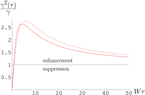
Figure 4: Projective measurements: $\gamma^{\mathrm{Z}}(\tau)/\gamma$ vs $W\tau$. Full line: exponential form factor (76); dashed line: polynomial form factor (77) with $n=2$.

The transition between these two regimes takes place at $\tau=\tau^{*}$, where $\tau^{*}$ is defined by the equation Heraclitus

$$\gamma^{\mathrm{Z}}(\tau^{*})=\gamma^{\mathrm{Z}}(\infty)=\gamma.$$ (139)

If $\tau^{*}$ belongs to the linear region (134) (which is our case and is true for sufficiently small energy $\Omega$ of the initial state), one gets

$$\tau^{*}\simeq\gamma\tau_{\mathrm{Z}}^{2}=2\pi\frac{\kappa^{\beta}(\Omega)}{\int_{-\infty}^{\infty}d\omega\;\kappa^{\beta}(\omega)}.$$ (140)

The short time region is displayed for clarity in Fig. 5.

It is useful to spend a few words on the physical meaning of the expressions $\tau\to 0$, $\beta\to\infty$ in the above (and following) formulas. Times and temperatures are to be compared with the bandwidth $W$ (or frequency cutoff $\Lambda$). Times (temperatures) are “small” when $\tau\ll W^{-1}$ ($\beta^{-1}\ll W$). For example, it is worth emphasizing that the relevant timescale is $\tau^{*}$, when one considers short-time expansions in a Zeno context Heraclitus ; Antoniou : the expansion (134) is valid for $\tau\lesssim W^{-1}$ (and not $\tau\lesssim\tau_{\rm Z}$, as it is sometimes erroneously assumed).

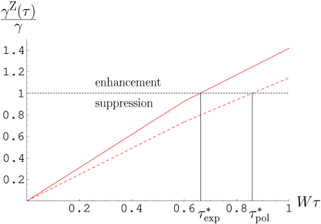
Figure 5: Projective measurements: $\gamma^{\mathrm{Z}}(\tau)/\gamma$ vs $W\tau$, for small $\tau$. Full line: exponential form factor (76); dashed line: polynomial form factor (77) with $n=2$. $\tau^{*}$ (indicated) is defined by the equation $\gamma^{\mathrm{Z}}(\tau^{*})/\gamma=1$. Decoherence is suppressed when $\gamma^{\mathrm{Z}}(\tau)<\gamma$; it is enhanced otherwise.

VII.2 “Bang bang” Control

We now discuss BB. The decay rate is given by Eq. (110):

$$\gamma^{\mathrm{k}}(\tau) = \frac{2}{\pi}\sum_{j=0}^{\infty}\frac{1}{\left(j+\frac{1}{2}\right)^{2}}\left[\kappa^{\beta}\left(\Omega+\frac{\pi}{\tau}(2j+1)\right)+\kappa^{\beta}\left(\Omega-\frac{\pi}{\tau}(2j+1)\right)\right]$$ (141)

$$\stackrel{{\scriptstyle\tau\to 0}}{{\thicksim}} \frac{2}{\pi}\sum_{j=0}^{\infty}\frac{1}{\left(j+\frac{1}{2}\right)^{2}}\;\kappa^{\beta}\left(\frac{\pi}{\tau}(2j+1)\right)\left(1+e^{-\beta\frac{\pi}{\tau}(2j+1)}\right)\thicksim\frac{2}{\pi}\sum_{j=0}^{\infty}\frac{1}{\left(j+\frac{1}{2}\right)^{2}}\;\kappa\left(\frac{\pi}{\tau}(2j+1)\right),$$

where we made use of (73) in the first expansion and assumed that $\beta$ is not too small (as compared to $\tau$) in the second one. In the exponential case (76) one gets

$$\kappa^{(E)}\left(\frac{\pi}{\tau}(2j+1)\right)=g^{2}\frac{\pi}{\tau}(2j+1)e^{-\frac{\pi}{\tau\Lambda}(2j+1)}=\kappa^{(E)}\left(\frac{\pi}{\tau}\right)(2j+1)e^{-2j\frac{\pi}{\tau\Lambda}}\ ,$$ (142)

whence

$$\gamma^{\mathrm{k}}(\tau)\sim\frac{8}{\pi}\,\kappa^{(E)}\left(\frac{\pi}{\tau}\right),\qquad\tau\to 0\ ,$$ (143)

while in the polynomial case (77) one gets

$$\kappa^{(P)}\left(\frac{\pi}{\tau}(2j+1)\right)\sim g^{2}\frac{\Lambda}{\left[\frac{\pi}{\tau\Lambda}(2j+1)\right]^{2n-1}}\sim\kappa^{(P)}\left(\frac{\pi}{\tau}\right)\frac{1}{(2j+1)^{2n-1}}\ ,$$ (144)

whence

$$\gamma^{\mathrm{k}}(\tau)\sim\frac{8}{\pi}\sum_{j=0}^{\infty}\frac{1}{(2j+1)^{2n+1}}\,\kappa^{(P)}\left(\frac{\pi}{\tau}\right)=\frac{8}{\pi}\left(1-2^{-2n-1}\right)\zeta(2n+1)\,\kappa^{(P)}\left(\frac{\pi}{\tau}\right),\qquad\tau\to 0,$$ (145)

where $\zeta(x)=\sum_{k=1}^{\infty}k^{-x}$ is the Riemann zeta function.

On the other hand, in both cases,

$$\gamma^{\mathrm{k}}(\tau)\to\frac{4}{\pi}\,\kappa^{\beta}\left(\Omega\right)\sum_{j=0}^{\infty}\frac{1}{\left(j+\frac{1}{2}\right)^{2}}=\gamma,\qquad\tau\to\infty,$$ (146)

where we summed the series

$$\sum_{j=0}^{\infty}\frac{1}{\left(j+\frac{1}{2}\right)^{2}}=4\sum_{j=0}^{\infty}\frac{1}{\left(2j+1\right)^{2}}=3\,\zeta(2)=\frac{\pi^{2}}{2}\ .$$ (147)

The ratio $\gamma^{\mathrm{k}}(\tau)/\gamma$ is shown in Fig. 6 as a function of $\tau$.

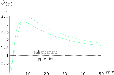
Figure 6: BB kicks: $\gamma^{\mathrm{k}}(\tau)/\gamma$ vs $W\tau$. Full line: exponential form factor (76); dashed line: polynomial form factor (77) with $n=2$.

Once again, the transition between the two regimes takes place at $\tau=\tau^{*}$ where $\tau^{*}$ is defined by the equation

$$\gamma^{\mathrm{k}}(\tau^{*})=\gamma^{\mathrm{k}}(\infty)=\gamma.$$ (148)

If $\tau^{*}$ is in the asymptotic region (143) one gets in the exponential case (76),

$$\kappa^{(E)}\left(\frac{\pi}{\tau^{*}}\right)\simeq\frac{\pi}{8}\gamma=\frac{\pi^{2}}{4}\kappa^{\beta}(\Omega),$$ (149)

which yields

$$\tau^{*}\simeq-\frac{\pi}{\Lambda}\,W_{-1}\left(-\frac{\pi}{8}\frac{\gamma}{g^{2}\Lambda}\right)^{-1}=-\frac{\pi}{\Lambda}\,W_{-1}\left(-\frac{\pi^{2}}{4}\frac{\kappa^{\beta}(\Omega)}{g^{2}\Lambda}\right)^{-1},$$ (150)

where $W$ is Lambert’s $W$-function Lambertfun , that is the inverse of the function $f(W)=We^{W}$, and we have taken its $-1$ branch.

On the other hand, for the polynomial case (77) one gets from (145)

$$\kappa^{(P)}\left(\frac{\pi}{\tau^{*}}\right)\simeq\frac{\pi}{8\left(1-2^{-2n-1}\right)\zeta(2n+1)}\gamma=\frac{\pi^{2}}{4\left(1-2^{-2n-1}\right)\zeta(2n+1)}\kappa^{\beta}(\Omega),$$ (151)

and

$$\tau^{*}\simeq\frac{\pi}{\Lambda}\,\left(\frac{\pi}{8\left(1-2^{-2n-1}\right)\zeta(2n+1)}\frac{\gamma}{g^{2}\Lambda}\right)^{\frac{1}{2n-1}}=\frac{3\pi}{\Lambda}\,\left(\frac{\pi^{2}}{4\left(1-2^{-2n-1}\right)\zeta(2n+1)}\frac{\kappa^{\beta}(\Omega)}{g^{2}\Lambda}\right)^{\frac{1}{2n-1}}\ .$$ (152)

The short-time region is shown in Fig. 7.

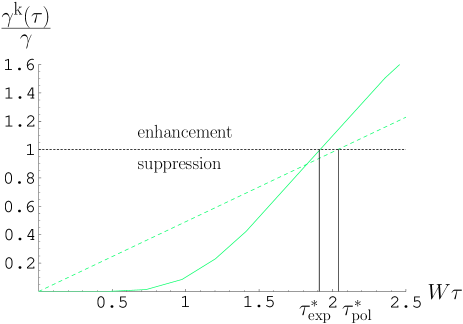
Figure 7: BB kicks: $\gamma^{\mathrm{k}}(\tau)/\gamma$ vs $W\tau$ for small $\tau$. Full line: exponential form factor (76); dashed line: polynomial form factor (77) with $n=2$. Decoherence is suppressed when $\gamma^{\mathrm{k}}(\tau)<\gamma$; it is enhanced otherwise.

It is useful to observe that the results (149)-(150) and (151)-(152) bear an important dependence of $\tau^{*}$ on the “tail” of the form factor. This is to be sharply contrasted with the projective measurement situation (140), that yields a dependence of the transition time $\tau^{*}$ on the “global” features of the form factor. This difference is apparent if one compares Figs. 5 and 7 and shows that the latter method offers important advantages if one aims at inhibiting decoherence, because of the larger (and easier to attain) value of $\tau^{*}$.

VII.3 Control by continuous coupling

Finally, we can look at continuous coupling. The timescale for decoherence is (133):

$$\gamma^{\mathrm{c}}(K) = \pi\int_{-\infty}^{\infty}d\omega\;\kappa^{\beta}(\omega)\;\left[\delta(\omega-\Omega-K)+\delta(\omega-\Omega+K)\right]$$ (153)

$$= \pi\left[\kappa^{\beta}(\Omega+K)+\kappa^{\beta}(\Omega-K)\right]\sim\pi\kappa(K)\left(1+e^{-\beta K}\right)\sim\pi\kappa(K),\qquad K\to\infty.$$

On the other hand,

$$\gamma^{\mathrm{c}}(K)\to\gamma,\qquad K\to 0.$$ (154)

Notice that the role of $K$ in Eq. (153) and the role of $1/\tau$ in Eqs. (143) and (145) are equivalent (see also Appendix C). This yields a natural comparison bang between different timescales ($\tau$ for measurements and kicks, $1/K$ for continuous coupling).

The ratio $\gamma^{\mathrm{c}}(K)/\gamma$ is shown in Fig. 8 as a function of $2\pi/K$.

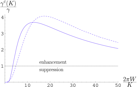
Figure 8: Continuous coupling: $\gamma^{\mathrm{c}}(K)/\gamma$ vs $2\pi W/K$. Full line: exponential form factor (76); dashed line: polynomial form factor (77) with $n=2$.

The transition between these two regimes takes now place at $K=K^{*}$ where $K^{*}$ is defined by the equation

$$\gamma^{\mathrm{c}}(K^{*})=\gamma^{\mathrm{c}}(0)=\gamma.$$ (155)

If $K^{*}$ is in the asymptotic region (153)

$$\kappa(K^{*})\simeq\frac{\gamma}{\pi}=2\kappa^{\beta}(\Omega).$$ (156)

For the exponential form factor (76) one gets

$$K^{*}\simeq-\Lambda\,W_{-1}\left(-\frac{1}{\pi}\frac{\gamma}{g^{2}\Lambda}\right)=-\Lambda\,W_{-1}\left(-2\frac{\kappa^{\beta}(\Omega)}{g^{2}\Lambda}\right),$$ (157)

while for the polynomial form factor (77) one gets

$$K^{*}\simeq\Lambda\,\left(\frac{1}{\pi}\frac{\gamma}{g^{2}\Lambda}\right)^{-\frac{1}{2n-1}}=\Lambda\,\left(2\frac{\kappa^{\beta}(\Omega)}{g^{2}\Lambda}\right)^{-\frac{1}{2n-1}}\ .$$ (158)

One observes a dependence of $K^{*}$ on the tail of the form factor. The strong coupling region is shown in Fig. 9.

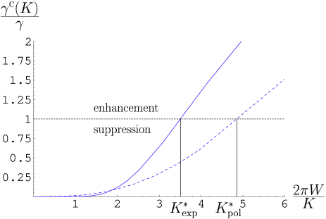
Figure 9: Continuous coupling: $\gamma^{\mathrm{c}}(K)/\gamma$ vs $2\pi W/K$ for large $K$. Full line: exponential form factor (76); dashed line: polynomial form factor (77) with $n=2$. Decoherence is suppressed when $\gamma^{\mathrm{c}}(K)<\gamma$; it is enhanced otherwise.

VII.4 Comparison among the three control strategies

There is a clear difference between bona fide projective measurements and the other two cases, BB kicks and continuous coupling. In the former case Eqs. (139)-(140) yield a dependence of $\tau^{*}$ on the global features of the form factor (i.e., its integral). By contrast, Eqs. (149)-(152) and (156)-(158) “pick” some particular (“on-shell”) value(s). This important difference, due to the different features of the evolution (non-unitary in the first case, unitary in the latter cases), is graphically displayed in Fig. 10 and 11, where the different mechanisms of control are compared. In Fig. 10, $\tau$ is “large” (in units of inverse bandwidth) and the three methods yield almost no control: one essentially reobtains the Fermi Golden rule $\gamma=2\pi\kappa^{\beta}(\Omega)$, although in different ways. In Fig. 11, $\tau$ is “small” and the effective lifetime is sensibly modified, although by different mechanisms.

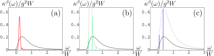
Figure 10: Different features of the three control methods. Form factor (polynomial, $n=2$) $\kappa^{\beta}(\omega)$ (dashed line) and form factor modulated/multiplied by the control “response” function (full line) for: (a) pulsed measurements, Eq. (134), with control response function $\tau{\rm sinc}^{2}[(\omega-\Omega)\tau/2]$ (here and in the other two cases, $\Omega=0.2W$); (b) BB kicks, Eq. (141), with control response function $(2/\pi)\sum_{j=0}^{\infty}\left(j+\frac{1}{2}\right)^{-2}\left[\delta\left(\omega-\Omega-\frac{\pi}{\tau}(2j+1)\right)+\delta\left(\omega-\Omega+\frac{\pi}{\tau}(2j+1)\right)\right]$ [see (109) and notice that the first 2-3 terms of the series yield an excellent approximation]; (c) continuous measurement, Eq. (153), with control response function $\pi[\delta(\omega-\Omega-K)+\delta(\omega-\Omega+K)]$. The gray line is a guide for the eye and interpolates $(2/\pi)\left(j+\frac{1}{2}\right)^{-2}\kappa^{\beta}(\omega)$ in (b) and $\pi\kappa^{\beta}(\omega)$ in (c). We set $\tau=2\pi/K=50W^{-1}$ (a “large” value): this yields in all cases a (controlled) decay rate that is very close to that obtained by the Fermi Golden rule.

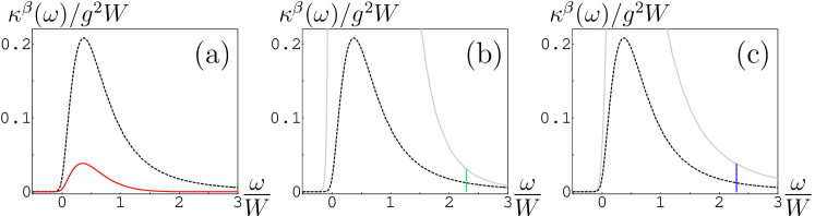
Figure 11: Same as in Fig. 10, but for $\tau=2\pi/K=3W^{-1}$ (a “small” value): this yields a bona fide control of the decay rate (in this particular situation, decoherence is enhanced in the Zeno case and suppressed in the other two cases). (a) The control response function $\tau{\rm sinc}^{2}[(\omega-\Omega)\tau/2]$ is very broad and the effective lifetime depends on the “global” features of the form factor. (b) For small $\tau$ all the arguments of the $\delta$-functions in (109) tend to $\infty$: for well-behaved form factors (like that shown in the figure), only the first term contributes significantly; the controlled lifetime depends on the local features of the “tail” of the form factor. (c) For large $K$ the arguments of the $\delta$-functions in Eq. (153) tend to $\pm\infty$ and the controlled lifetime depends again on the local features of the “tail” of the form factor.

The three control methods are graphically compared in Figs. 12-13. The different features discussed in Figs. 10-11 yield very different outputs, clearly apparent in Fig. 13, that can be important in practical applications: decoherence can be more easily halted by applying BB and/or continuous coupling strategies. These two methods yield values of $\tau^{*}$ (or $K^{*}$) that are easier to attain. However, this advantage has a price, because BB and continuous coupling yield a larger enhancement of decoherence for $\tau>\tau^{*}$, $K<K^{*}$. The two dynamical methods perform better only when $\tau\lesssim\tau^{*}$, $K\gtrsim K^{*}$. This is apparent in Fig. 12. We notice that a strict comparison between continuous coupling and the other two methods is difficult, as it would involve an analysis of numerical factors of order one in the definition of the relevant conversion factors between the frequency of interruptions $\tau$ and the coupling $K$ [this factor has been sensibly–but arbitrarily–set equal to $2\pi$ in Figs. 12-13: see sentence after Eq. (154) and Appendix C].

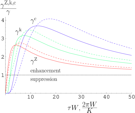
Figure 12: Comparison among the three control methods. The graphs of Figs. 4, 6 and 8 are displayed together. BB kicks and continuous coupling are more effective than bona fide measurements for combatting decoherence, as the regime of “suppression” is reached for larger values of $\tau$ and $K^{-1}$.

Figure 13: Comparison among the three control methods: small times/strong coupling regions. The graphs of Figs. 5, 7 and 9 are displayed together.

VIII SUMMARY AND CONCLUDING REMARKS

We have analyzed and compared three control methods for combatting decoherence. The first is based on repeated quantum measurements (projection operators) and involves a description in terms of nonunitary processes. The second and third methods are both dynamical, as they can be described in terms of unitary evolutions. In all cases, decoherence can be halted by very rapidly/strongly driving or very frequently measuring the system state. However, if the frequency is not high enough or the coupling not strong enough, the controls may accelerate the decoherence process and deteriorate the performance of the quantum state manipulation. The acceleration of decoherence is analogous to the inverse Zeno effect, namely the acceleration of the decay of an unstable state due to frequent measurements IZE ; Heraclitus .

As a general rule, when one endeavors to control decoherence by suitably tailoring the coupling of the system of interest to another system (such as an external field, or a measuring apparatus), one should carefully look at the relevant timescales, as it is not true that repeated measurements/interruptions always lead to a suppression of decoherence.

It is convenient to summarize the main results obtained in this article in the particular case of a two-level system (qubit) with energy difference $\Omega$. If the frequency $\tau^{-1}$ of measurements or BB kicks, or the strength $K$ of the coupling tend to $\infty$, the two-dimensional (Zeno) subspace defining the qubit becomes isolated and decoherence is completely suppressed. However, if $\tau^{-1}$ and $K$ are large, but not extremely large, the transition (decay) rates between the qubit subspace and the remaining sector of the Hilbert space display a complicated dependence on $\tau^{-1}$ and $K$, and decoherence can be suppressed or enhanced, depending on the situation.

At low temperature $\beta^{-1}\ll\Omega\ll W$, where $W$ is the bandwidth of the form factor of the interaction, the decay rates read, from (134), (135), (143), (145) and (153)

$$\left\{\begin{array}[]{l}\gamma^{Z}(\tau)\sim\frac{\tau}{\tau_{Z}^{2}},\qquad\tau\to 0\ ,\\ \\ \gamma^{\mathrm{k}}(\tau)\sim\frac{8}{\pi}\kappa\left(\frac{\pi}{\tau}\right),\qquad\tau\to 0\ ,\\ \\ \gamma^{\mathrm{c}}(K)\sim\pi\kappa(K),\qquad K\to\infty\ ,\end{array}\right.$$ (159)

where $Z$, k and c denote (Zeno) measurements, (BB) kicks and continuous coupling, respectively, $\kappa$ is the form factor and $1/\tau_{Z}^{2}\simeq\int d\omega\kappa(\omega)$ the Zeno time (more accurate definitions were given in the preceding sections). As we have shown, there is a characteristic transition time $\tau^{*}$ [coupling $K^{*}$], such that one obtains:

$$\mbox{decoherence suppression}: \gamma(\tau)<\gamma\quad[\gamma(K)<\gamma],\qquad\mbox{for}\quad\tau<\tau^{*}\quad[K>K^{*}],$$

$$\mbox{decoherence enhancement}: \gamma(\tau)>\gamma\quad[\gamma(K)>\gamma],\qquad\mbox{for}\quad\tau>\tau^{*}\quad[K<K^{*}].$$ (160)

Therefore, in order to obtain a suppression of decoherence, the interruptions/coupling must be very frequent/strong. Notice, in this context, that both $\tau^{*}$ and $2\pi/K^{*}$ are not simply related to the inverse bandwidth $2\pi W^{-1}$: they can be in general (much) shorter. For instance, in the Ohmic polynomial case (77), one easily gets from (78) and (159)

$$\left\{\begin{array}[]{l}\tau^{*}_{Z}\simeq 2\pi W^{-1}\left(2(n-1)\alpha_{n}^{2}\frac{\Omega}{W}\right)\ll 2\pi W^{-1}\ ,\\ \\ \tau^{*}_{\mathrm{k}}\simeq 2\pi W^{-1}\frac{\alpha_{n}}{2}\left(\frac{\alpha_{n}\pi^{2}}{4}\frac{\Omega}{W}\right)^{\frac{1}{2n-1}}\ll 2\pi W^{-1}\ ,\\ \\ K^{*}\simeq W\alpha_{n}^{-1}\left(\frac{2}{\alpha_{n}}\frac{W}{\Omega}\right)^{\frac{1}{2n-1}}\gg W\ ,\end{array}\right.$$ (161)

where $\alpha_{n}=(\sqrt{\pi}/2)\Gamma(n-3/2)/\Gamma(n-1)\leq\pi/2$ is a coefficient of order $1$ and $n$ characterizes the polynomial fall off of the form factor (77). The above times/coupling may be (very) difficult to achieve in practice. In fact, we see here that the relevant timescale is not simply the inverse bandwidth $2\pi W^{-1}$, but can be much shorter if $\Omega\ll W$, as is typically the case. These conclusions, summarized here for the simple case of a qubit, are valid in general, when one aims at protecting from decoherence an $N$-dimensional Hilbert subspace.

An important example that we have not explicitly analyzed in this article is the case of $1/f$ noise, and its suppression by means of techniques like those discussed here. There has recently been a surge of interest in this issue in quantum information processing devices, where such noise is often attributable to (but certainly not limited to) charge fluctuations in electrodes providing control voltages Galperin:03 ; Makhlin:03 . The need for such electrodes is widespread in quantum computer proposals, e.g., trapped ions (where observed $1/f$ noise was reported in Turchette:00 ), quantum dots Burkard:99 , doped silicon Kane:98 ; Vrijen:00 , electrons on helium Platzman:99 , and superconducting qubits Paladino:02 . In the latter case, in a recent experiment involving a charge qubit in a small superconducting electrode (Cooper-pair box), a spin-echo-type version of BB was successfully used to suppress low-frequency energy-level fluctuations (causing dephasing) due to $1/f$ charge noise Nakamura:02 . Several recent papers have dealt with suppression of this particular kind of noise via BB decoupling ShiokawaLidar ; Gutmann:03 ; Faoro:03 ; Falci:03 . The “bottom-up” approach models $1/f$ noise as arising from a collection of bi-stable fluctuators Gutmann:03 ; Faoro:03 ; Falci:03 ; Galperin:03 . The alternative is to treat $1/f$ noise as contributing a particular form factor ShiokawaLidar ; Makhlin:03 . We will pursue these ideas as a future topic of investigation, but we expect that the main results obtained in the present paper be applicable to this case as well.

The results obtained in this paper are of general validity and bring to light the different features of the control procedures as well as the crucial role played by the form factor of the interaction. We do not expect any drastic change for different decoherence mechanisms and/or different physical systems. The only somewhat delicate issue, in our opinion, is to understand whether the system investigated can be consistently described by means of a set of discrete levels.

Appendix A

In this Appendix, the assumption of the factorized form of the initial density operator, as in (5), which is usually taken for granted, is shown to be justified in the weak-coupling (scaling) limit. We only outline the main derivation. Further details will be reported elsewhere factorassumption .

Consider the initial-value problem

$${\partial\over\partial t}\rho={\mathcal{L}}_{\mathrm{tot}}\rho=({\mathcal{L}}_{0}+\lambda{\mathcal{L}}_{SB})\rho=({\mathcal{L}}_{S}+{\mathcal{L}}_{B}+\lambda{\mathcal{L}}_{SB})\rho,\quad\rho(0)=\rho_{0},$$ (162)

where the dependence on the coupling constant $\lambda$ of the interaction Liouvillian ${\mathcal{L}}_{SB}$ is made explicit. Notice that the initial density operator can be of any form and is not assumed here to be factorized like in (5). The projection operators $\mathcal{P}$ and $\mathcal{Q}$, defined in (41), and the above Liouvillians ${\mathcal{L}}_{S},\,{\mathcal{L}}_{B}$ and ${\mathcal{L}}_{SB}$ satisfy the same conditions (42) and (43). The projected density operators $\mathcal{P}\rho$ and $\mathcal{Q}\rho$ satisfy

$${\partial\over\partial t}{\mathcal{P}}\rho={\mathcal{L}}_{0}{\mathcal{P}}\rho+\lambda{\mathcal{P}}{\mathcal{L}}_{SB}{\mathcal{Q}}\rho,\qquad{\partial\over\partial t}{\mathcal{Q}}\rho=({\mathcal{L}}_{0}+\lambda{\mathcal{Q}}{\mathcal{L}}_{SB}{\mathcal{Q}}){\mathcal{Q}}\rho+\lambda{\mathcal{Q}}{\mathcal{L}}_{SB}{\mathcal{P}}\rho,$$ (163)

respectively. Following the same procedure as in Sec. III, we arrive at the following exact equation for the ${\mathcal{P}}$-projected operator in the interaction picture

$${\partial\over\partial t}\left(e^{-{\mathcal{L}}_{0}t}{\mathcal{P}}\rho\right) = \lambda e^{-{\mathcal{L}}_{0}t}{\mathcal{P}}{\mathcal{L}}_{SB}e^{({\mathcal{L}}_{0}+\lambda{\mathcal{Q}}{\mathcal{L}}_{SB}{\mathcal{Q}})t}{\mathcal{Q}}\rho_{0}$$ (164)

$$+\lambda^{2}\int_{0}^{t}dt^{\prime}e^{-{\mathcal{L}}_{0}t}{\mathcal{P}}{\mathcal{L}}_{SB}e^{({\mathcal{L}}_{0}+\lambda{\mathcal{Q}}{\mathcal{L}}_{SB}{\mathcal{Q}})t^{\prime}}{\mathcal{L}}_{SB}{\mathcal{P}}\rho(t-t^{\prime}).$$

Notice that the first term on the rhs represents the contribution arising from a possible initial correlation between the system and reservoir. We now show that this term dies out in the weak-coupling (i.e., scaling) limit $\lambda\to 0$ with fixed $\tau\equiv\lambda^{2}t$. For this purpose, define

$$\rho_{\mathrm{I}}(\tau;\lambda)\equiv e^{-{\mathcal{L}}_{0}\tau/\lambda^{2}}{\mathcal{P}}\rho(\tau/\lambda^{2}),$$ (165)

that satisfies

$$\dot{\rho}_{\mathrm{I}}(\tau;\lambda) = {1\over\lambda}e^{-{\mathcal{L}}_{0}\tau/\lambda^{2}}{\mathcal{P}}{\mathcal{L}}_{SB}e^{({\mathcal{L}}_{0}+\lambda{\mathcal{Q}}{\mathcal{L}}_{SB}{\mathcal{Q}})\tau/\lambda^{2}}{\mathcal{Q}}\rho_{0}$$ (166)

$$+\int_{0}^{\tau/\lambda^{2}}dt^{\prime}e^{-{\mathcal{L}}_{0}\tau/\lambda^{2}}{\mathcal{P}}{\mathcal{L}}_{SB}e^{({\mathcal{L}}_{0}+\lambda{\mathcal{Q}}{\mathcal{L}}_{SB}{\mathcal{Q}})t^{\prime}}{\mathcal{L}}_{SB}e^{{\mathcal{L}}_{0}(\tau/\lambda^{2}-t^{\prime})}{\mathcal{P}}\rho_{\mathrm{I}}(\tau-\lambda^{2}t^{\prime};\lambda).$$

The first term vanishes in the $\lambda\to 0$ limit factorassumption , since

$$\int_{0}^{\infty}d\tau{1\over\lambda}e^{\mathcal{A}\tau/\lambda^{2}}Y(\tau)=\lambda\int_{0}^{\infty}d\tau e^{\mathcal{A}\tau}Y(\lambda^{2}\tau)\longrightarrow 0,\quad\hbox{as }\quad\lambda\to 0,$$ (167)

for any superoperator such that the integral $\int_{0}^{\infty}d\tau e^{\mathcal{A}\tau}$ exists. This means that the contribution originating from the initial correlation between the system and reservoir disappears in the scaling limit and therefore we are allowed to start from an initial density matrix in the factorized form (5).

Finally, the dynamics of $\rho_{\mathrm{I}}(\tau;0)$ is governed by

$$\dot{\rho}_{\mathrm{I}}(\tau;0)=\sum_{\omega}\tilde{Q}_{\omega}\int_{0}^{\infty}dt^{\prime}{\mathcal{P}}{\mathcal{L}}_{SB}(0){\mathcal{Q}}{\mathcal{L}}_{SB}(-t^{\prime})\tilde{Q}_{\omega}\rho_{\mathrm{I}}(\tau;0)$$ (168)

with the factorized initial condition (5), where the $\tilde{Q}_{\omega}$ are the eigenprojections of the Liouvillian ${\mathcal{L}}_{S}$ defined in (52).

From a physical point of view, the factorization ansatz described in this appendix simply means that the “initial” correlations between the system and its environment are “forgotten” on a time scale of order $\lambda^{2}$. We also note that several authors have addressed the question of the modifications that arise when it is not permissible to assume initially separable system-environment, e.g., factorvari .

Appendix B

We derive Eq. (87). The first equality reads

$$\left[{\hat{P}}e^{{\mathcal{L}}_{\rm tot}\tau}{\hat{P}}\right]^{t/\tau}\simeq\left[{\hat{P}}V_{Z}(\tau){\hat{P}}\right]^{t/\tau},\qquad V_{Z}(\tau)=e^{{\mathcal{L}}_{0}\tau}{\cal T}\exp\left(\int_{0}^{\tau}ds\;e^{-{\mathcal{L}}_{0}s}{\mathcal{G}}_{\mathrm{Z}}(\tau)e^{{\mathcal{L}}_{0}s}\right).$$ (169)

Let us write $V_{Z}(\tau)=V(\tau,\tau)$, where

$$V(t,u)=e^{{\mathcal{L}}_{0}t}{\cal T}\exp\left(\int_{0}^{t}ds\;e^{-{\mathcal{L}}_{0}s}{\mathcal{G}}_{\mathrm{Z}}(u)e^{{\mathcal{L}}_{0}s}\right).$$ (170)

By deriving with respect to $t$, we get

$$\partial_{t}V(t,u)=[{\mathcal{L}}_{0}+{\mathcal{G}}_{\mathrm{Z}}(u)]V(t,u),$$ (171)

so that

$$V(t,u)=\exp\{[{\mathcal{L}}_{0}+{\mathcal{G}}_{\mathrm{Z}}(u)]t\},$$ (172)

where we used $V(0,u)=1$. As a consequence, $V_{Z}(\tau)=\exp\{[{\mathcal{L}}_{0}+{\mathcal{G}}_{\mathrm{Z}}(\tau)]\tau\}$ and

$$\left[{\hat{P}}e^{{\mathcal{L}}_{\rm tot}\tau}{\hat{P}}\right]^{t/\tau}\simeq\left[{\hat{P}}\exp\{[{\mathcal{L}}_{0}+{\mathcal{G}}_{\mathrm{Z}}(\tau)]\tau\}{\hat{P}}\right]^{t/\tau}={\hat{P}}\exp\{[{\mathcal{L}}_{0}+{\mathcal{G}}_{\mathrm{Z}}(\tau)]t\},$$ (173)

because $[\hat{P},{\mathcal{L}}_{0}]=[\hat{P},{\mathcal{G}}_{\mathrm{Z}}]=0$. This is Eq. (87).

Let us now solve Eq. (89):

$$\int_{0}^{\tau}dt\;e^{-{\mathcal{L}}_{S}t}{\mathcal{L}}_{\mathrm{Z}}(\tau)e^{{\mathcal{L}}_{S}t}=\int_{0}^{\tau}dt{\hat{P}}{\mathcal{L}}_{\mathrm{I}}(t){\hat{P}}=\int_{0}^{\tau}dt\int_{0}^{t}ds\;{\hat{P}}{\mathcal{K}}_{\mathrm{I}}(t,s){\hat{P}}\ .$$ (174)

By using (48) and (44)

$${\mathcal{K}}_{\mathrm{I}}(t,s)\,\sigma=\mathrm{tr}_{B}\left\{{\mathcal{L}}_{SB}(t){\mathcal{L}}_{SB}(s)\,\sigma\otimes\rho_{B}\right\},\qquad{\mathcal{L}}_{SB}(t)=e^{-({\mathcal{L}}_{S}+{\mathcal{L}}_{B})t}{\mathcal{L}}_{SB}e^{({\mathcal{L}}_{S}+{\mathcal{L}}_{B})t},$$ (175)

we get

$$\int_{0}^{\tau}dt\;e^{-{\mathcal{L}}_{S}t}{\mathcal{L}}_{\mathrm{Z}}(\tau)e^{{\mathcal{L}}_{S}t}\sigma = \int_{0}^{\tau}dt\int_{0}^{t}ds\;\mathrm{tr}_{B}\left\{{\hat{P}}{\mathcal{L}}_{SB}(t){\mathcal{L}}_{SB}(s)\,{\hat{P}}\sigma\otimes\rho_{B}\right\}$$ (176)

$$= \int_{0}^{\tau}dt\;e^{-{\mathcal{L}}_{S}t}\int_{-t}^{0}ds\;\mathrm{tr}_{B}\left\{{\hat{P}}{\mathcal{L}}_{SB}{\mathcal{L}}_{SB}(s){\hat{P}}e^{{\mathcal{L}}_{S}t}\sigma\otimes\rho_{B}\right\}.$$

Let us rewrite the previous equation in terms of the eigenprojections $\tilde{Q}_{\omega}$ of ${\mathcal{L}}_{S}$ defined by (52):

$$\sum_{\omega,\omega^{\prime}}\int_{0}^{\tau}dt\;e^{i(\omega-\omega^{\prime})t}\tilde{Q}_{\omega}{\mathcal{L}}_{\mathrm{Z}}(\tau)\tilde{Q}_{\omega^{\prime}}\sigma=\sum_{\omega,\omega^{\prime}}\int_{0}^{\tau}dt\;e^{i(\omega-\omega^{\prime})t}\int_{-t}^{0}ds\;\mathrm{tr}_{B}\left\{\tilde{Q}_{\omega}{\hat{P}}{\mathcal{L}}_{SB}{\mathcal{L}}_{SB}(s){\hat{P}}\tilde{Q}_{\omega^{\prime}}\sigma\otimes\rho_{B}\right\}.$$ (177)

Performing the first integral, we get

$$\tilde{Q}_{\omega}{\mathcal{L}}_{\mathrm{Z}}(\tau)\tilde{Q}_{\omega^{\prime}}\sigma=\frac{g((\omega-\omega^{\prime})\tau)}{\tau}\int_{0}^{\tau}dt\;e^{i(\omega-\omega^{\prime})t}\int_{-t}^{0}ds\;\mathrm{tr}_{B}\left\{\tilde{Q}_{\omega}{\hat{P}}{\mathcal{L}}_{SB}{\mathcal{L}}_{SB}(s){\hat{P}}\tilde{Q}_{\omega^{\prime}}\sigma\otimes\rho_{B}\right\},\qquad g(x)=\frac{ix}{e^{ix}-1}.$$ (178)

Since $g(0)=1$, the diagonal terms yield

$$\tilde{Q}_{\omega}{\mathcal{L}}_{\mathrm{Z}}(\tau)\tilde{Q}_{\omega}\sigma=\frac{1}{\tau}\int_{0}^{\tau}dt\int_{-t}^{0}ds\;\mathrm{tr}_{B}\left\{\tilde{Q}_{\omega}{\hat{P}}{\mathcal{L}}_{SB}{\mathcal{L}}_{SB}(s){\hat{P}}\tilde{Q}_{\omega}\sigma\otimes\rho_{B}\right\}.$$ (179)

The off-diagonal terms do not contribute to the master equation, as explained at the end of Sec. III, Eqs. (50)-(55).

By using the property (64) and noting that $[\hat{P},\tilde{Q}_{\omega}]=0$ by (15), we get

$${\mathcal{L}}_{\mathrm{Z}}(\tau)\sigma=-\sum_{\omega}\frac{1}{\tau}\int_{0}^{\tau}dt\int_{-t}^{0}ds\;\mathrm{tr}_{B}\left\{{\hat{P}}\left[\left(\tilde{Q}_{\omega}H_{SB}\right),\left[\left(\tilde{Q}_{-\omega}H_{SB}(s)\right),{\hat{P}}\sigma\otimes\rho_{B}\right]\right]\right\},$$ (180)

whence, by using (66),

$${\mathcal{L}}_{\mathrm{Z}}(\tau)\sigma = -\sum_{m}\frac{1}{\tau}\int_{0}^{\tau}dt\int_{-t}^{0}ds\;\mathrm{tr}_{B}\left\{{\hat{P}}\left[H_{SB}^{(m)},\left[H_{SB}^{(-m)}(s),{\hat{P}}\sigma\otimes\rho_{B}\right]\right]\right\}$$ (181)

$$= -\sum_{m}\frac{1}{\tau}\int_{0}^{\tau}dt\int_{-t}^{0}ds\;\mathrm{tr}_{B}\left\{{\hat{P}}\left[X^{\dagger}_{m}\otimes A_{m},\left[X_{m}\otimes A^{\dagger}_{m}(s),{\hat{P}}\sigma\otimes\rho_{B}\right]\right]\right.$$

$$\qquad\qquad\qquad\qquad\qquad\quad\left.+{\hat{P}}\left[X_{-m}\otimes A^{\dagger}_{-m},\left[X^{\dagger}_{-m}\otimes A_{-m}(s),{\hat{P}}\sigma\otimes\rho_{B}\right]\right]\right\},$$

where, like in Eq. (67), in the second equality we neglected terms containing two annihilation or creation operators. From (181) we get Eq. (LABEL:eq:disscLz) with

$$\gamma_{m}^{\mathrm{Z}}(\tau)=\frac{2}{\tau}\mathrm{\,Re}\int_{0}^{\tau}dt\int_{-t}^{0}ds\left(\left\langle A_{m}(0)A^{\dagger}_{m}(s)\right\rangle+\left\langle A_{-m}^{\dagger}(0)A_{-m}(s)\right\rangle\right).$$ (182)

By noticing that

$$\left\langle A_{m}A^{\dagger}_{m}(s)\right\rangle+\left\langle A_{-m}^{\dagger}A_{-m}(s)\right\rangle=\int_{-\infty}^{\infty}d\omega\;\kappa^{\beta}_{m}(\omega)e^{i(\omega-\omega_{m})s},$$ (183)

we finally get

$$\gamma_{m}^{\mathrm{Z}}(\tau)=\frac{2}{\tau}\int_{-\infty}^{\infty}d\omega\;\kappa^{\beta}_{m}(\omega)\frac{1-\cos(\omega-\omega_{m})\tau}{(\omega-\omega_{m})^{2}}=\tau\int_{-\infty}^{\infty}d\omega\;\kappa^{\beta}_{m}(\omega)\frac{\sin^{2}\left(\frac{\omega-\omega_{m}}{2}\tau\right)}{\left(\frac{\omega-\omega_{m}}{2}\tau\right)^{2}},$$ (184)

which is Eq. (92) of the text.

Appendix C

We derive Eqs. (101) and (103). We start from Eqs. (95) and (96)

$$\int_{0}^{\tau}ds\;e^{-{\mathcal{L}}_{\tau}s}{\mathcal{F}}_{\mathrm{k}}(\tau)e^{{\mathcal{L}}_{\tau}s}=\int_{0}^{\tau}ds\;{\mathcal{L}}_{SB}(s)\ ,$$ (185)

$$\int_{0}^{\tau}ds\;e^{-{\mathcal{L}}_{\tau}s}{\mathcal{G}}_{\mathrm{k}}(\tau)e^{{\mathcal{L}}_{\tau}s}=\int_{0}^{\tau}ds\int_{0}^{s}ds_{1}\;\left[{\mathcal{L}}_{SB}(s){\mathcal{L}}_{SB}(s_{1})-e^{-{\mathcal{L}}_{\tau}s}{\mathcal{F}}_{\mathrm{k}}(\tau)e^{{\mathcal{L}}_{\tau}(s-s_{1})}{\mathcal{F}}_{\mathrm{k}}(\tau)e^{{\mathcal{L}}_{\tau}s_{1}}\right]\ ,$$ (186)

where ${\mathcal{L}}_{\tau}=\frac{{\mathcal{L}}_{\mathrm{k}}}{\tau}+{\mathcal{L}}_{0}$, and by taking the trace over the bath we get

$$\int_{0}^{\tau}dt\;e^{-{\mathcal{L}}^{\prime}_{S}t}{\mathcal{L}}_{k}(\tau)e^{{\mathcal{L}}^{\prime}_{S}t}\sigma=\int_{0}^{\tau}dt\int_{-t}^{0}ds\;\mathrm{tr}_{B}\left\{\left[e^{-{\mathcal{L}}_{S}t}{\mathcal{L}}_{SB}{\mathcal{L}}_{SB}(s)-e^{-{\mathcal{L}}^{\prime}_{S}t}{\mathcal{F}}_{\mathrm{k}}(\tau)e^{-{\mathcal{L}}_{\tau}s}{\mathcal{F}}_{\mathrm{k}}(\tau)e^{{\mathcal{L}}_{\tau}s}e^{{\mathcal{L}}^{\prime}_{S}t}\right]\sigma\otimes\rho_{B}\right\},$$ (187)

with

$${\mathcal{L}}_{S}(\tau)=\frac{{\mathcal{L}}_{\mathrm{k}}}{\tau}+{\mathcal{L}}_{S}.$$ (188)

Equation (187) is similar to (176) and, by projecting onto the eigenprojections $\tilde{P}_{\omega}(\tau)$ of ${\mathcal{L}}_{S}(\tau)$ and taking only the diagonal terms, one obtains Eq. (101). However, in order to compute the decay rates $\gamma_{m}^{\mathrm{k}}(\tau)$ one can give an alternative, more physical derivation by elaborating on the technique of Ref. bang . First notice that the BB dynamics (93) is generated by the time-dependent Hamiltonian

$$H\left(t/\tau\right)=H_{\mathrm{tot}}+H_{\mathrm{k}}\;\delta_{P}\left(t/\tau\right),\quad\delta_{P}(x)=\sum_{n\in\mathbb{Z}}\delta(x-n)\ .$$ (189)

In the enlarged Hilbert space $\mathcal{H}\otimes L^{2}(\mathbb{T})$ we can consider the (time-independent) Floquet Hamiltonian

$$H_{\mathrm{Floq}}=H(\theta)+\frac{1}{\tau}p_{\theta}=H_{\mathrm{tot}}+H_{\mathrm{k}}\delta_{P}(\theta)+\frac{1}{\tau}p_{\theta},$$ (190)

where

$$\theta\in\left[-1/2,1/2\right),\quad p_{\theta}=-i\partial_{\theta},\quad\left[\theta,p_{\theta}\right]=i.$$ (191)

We get

$$\dot{\theta}=-i\left[\theta,H_{\mathrm{Floq}}\right]=1/\tau,\qquad\theta(t)=t/\tau,$$ (192)

whence $\forall A\in\mathcal{H}$,

$$\dot{A}(t)=-i\left[A(t),H_{\mathrm{Floq}}\right]=-i\left[A(t),H\left(t/\tau\right)\right],$$ (193)

so that every observable in $\mathcal{H}$ evolves according to the original Hamiltonian (189). The eigenvalue equation for $p_{\theta}$ reads

$$p_{\theta}|m\rangle=2\pi m|m\rangle,\qquad\langle\theta|m\rangle=e^{i2\pi m\theta},\quad m\in\mathbb{Z}.$$ (194)

The Hamiltonian (190) in $\mathcal{H}\otimes L^{2}(\mathbb{T})$ represents a control by a strong continuous coupling, analogous to that discussed in Sec. VI, if one identifies $K=1/\tau$ and $H_{c}=p_{\theta}$. Therefore, from Eq. (122) and (194) we obtain

$$\omega_{mn}(\tau) = \frac{1}{\tau}\Omega_{m}+\Omega_{mn}^{(1)}+{\rm O}\left(\tau\right)=\frac{2\pi m}{\tau}+\Omega_{mn}^{(1)}+{\rm O}\left(\tau\right)\ ,$$ (195)

and from Eq. (119) we get

$$\gamma_{mn}^{\mathrm{k}}(\tau)=2\pi\kappa_{n}^{\beta}\left(\omega_{mn}(\tau)\right)=2\pi\kappa_{n}^{\beta}\left(\frac{2\pi m}{\tau}+\Omega^{(1)}_{mn}+\mathrm{O}(\tau)\right)\ ,$$ (196)

which is Eq. (103) of the text.

References

- (1) D. Giulini, E. Joos, C. Kiefer, J. Kupsch, I.-O. Stamatescu, and H.-D. Zeh, Decoherence and the Appearance of a Classical World in Quantum Theory (Springer, Berlin, 1996); M. Namiki, S. Pascazio and H. Nakazato, Decoherence and Quantum Measurements (World Scientific, Singapore, 1997).
- (2) A. Galindo and M.A. Martin-Delgado, Rev. Mod. Phys. 74, 347 (2002); D. Bouwmeester, A. Ekert and A. Zeilinger, Eds. The Physics of Quantum Information (Springer, Berlin, 2000); M.A. Nielsen and I.L. Chuang, Quantum Computation and Quantum Information (Cambridge University Press, Cambridge, 2000).
- (3) W.G. Unruh, Phys. Rev.A 51, 992 (1995). See also I.L. Chuang, R. Laflamme, P.W. Shor, W.H. Zurek, Science 270, 1633 (1995).
- (4) P.W. Shor, Phys. Rev. A 52, 2493 (1995); A.R. Calderbank and P.W. Shor, Phys. Rev. A 54, 1098 (1996); A. Steane, Proc. R. Soc. London A 452, 2551 (1996); A. Steane, Phys. Rev. Lett. 77, 793 (1996). For a review, see J. Preskill, in Introduction to Quantum Computation and Information, edited by H.K. Lo, S. Popescu, T.P. Spiller (World Scientific, Singapore, 1999).
- (5) S. Mancini and R. Bonifacio, Phys. Rev. A 64, 042111 (2001); S. Mancini, D. Vitali, P. Tombesi and R. Bonifacio, Europhys. Lett. 60, 498 (2002); S. Mancini, D. Vitali, P. Tombesi and R. Bonifacio, J. Opt. B. 4, S300 (2002); H. Wiseman, S. Mancini and J. Wang, Phys. Rev. A 66, 013807 (2002).
- (6) G. M. Palma, K. A. Suominen and A. K. Ekert, Proc. R. Soc. Lond. A 452, 567 (1996); L.M. Duan and G.C. Guo, Phys. Rev. Lett. 79, 1953 (1997); P. Zanardi and M. Rasetti, Phys. Rev. Lett. 79, 3306 (1997); D.A. Lidar, I.L. Chuang and K.B. Whaley, Phys. Rev. Lett. 81, 2594 (1998); E. Knill, R. Laflamme and L. Viola, Phys. Rev. Lett. 84, 2525 (2000). For a review, see D.A. Lidar and K.B Whaley, “Decoherence-Free Subspaces and Subsystems,” in “Irreversible Quantum Dynamics,” F. Benatti and R. Floreanini (Eds.), p. 83 (Springer Lecture Notes in Physics vol. 622, Berlin, 2003) (quant-ph/0301032)
- (7) L. Viola and S. Lloyd, Phys. Rev. A 58, 2733 (1998).
- (8) L. Viola, E. Knill and S. Lloyd, Phys. Rev. Lett. 82, 2417 (1999); ibid. 83, 4888 (1999); ibid. 85, 3520 (2000).
- (9) P. Zanardi, Phys. Lett. A 258, 77 (1999).
- (10) D. Vitali and P. Tombesi, Phys. Rev. A 59, 4178 (1999); Phys. Rev. A 65, 012305 (2001); C. Uchiyama and M. Aihara, Phys. Rev. A 66, 032313 (2002).
- (11) M.S. Byrd and D.A. Lidar, Quantum Information Processing 1, 19 (2002); Phys. Rev. A 67, 012324 (2003).
- (12) P. Facchi, D.A. Lidar and S. Pascazio, Phys. Rev. A 69, 032314 (2004).
- (13) J. von Neumann, Mathematical Foundation of Quantum Mechanics (Princeton University Press, Princeton, 1955); A. Beskow and J. Nilsson, Arkiv für Fysik 34, 561 (1967); L.A. Khalfin, JETP Letters 8, 65 (1968).
- (14) B. Misra and E.C.G. Sudarshan, J. Math. Phys. 18, 756 (1977).
- (15) D. Home and M.A.B. Whitaker, Ann. Phys. 258, 237 (1997).
- (16) P. Facchi and S. Pascazio, Progress in Optics, ed. E. Wolf (Elsevier, Amsterdam, 2001), vol. 42, Chapter 3, p.147.
- (17) P. Facchi and S. Pascazio, Phys. Rev. Lett. 89 080401 (2002); “Quantum Zeno subspaces and dynamical superselection rules,” in “The Physics of Communication,” Proceedings of the XXII Solvay Conference in Physics, edited by I. Antoniou, V.A. Sadovnichy and H. Walther (World Scientific, Singapore, 2003) p. 251 (quant-ph/0207030).
- (18) P. Facchi, V. Gorini, G. Marmo, S. Pascazio and E.C.G. Sudarshan, Phys. Lett. A 275, 12 (2000); P. Facchi, S. Pascazio, A. Scardicchio and L.S. Schulman, Phys. Rev. A 65, 012108 (2002).
- (19) C.N. Friedman, Indiana Univ. Math. J. 21, 1001 (1972).
- (20) K. Gustafson, “Irreversibility questions in chemistry, quantum-counting, and time-delay.” In Energy storage and redistribution in molecules, ed. by J. Hinze (Plenum, 1983), and refs. [10,12] therein; K. Gustafson, “A Zeno story,” quant-ph/0203032.
- (21) P. Exner and T. Ichinose, “Product formula related to quantum Zeno dynamics,” math-ph/0302060.
- (22) A.U. Schmidt, J. Phys. A: Math. Gen. 35, 7817 (2002); ibid 36, 1135 (2003).
- (23) B. Misra and A. Antoniou, “Quantum Zeno effect,” in “The Physics of Communication,” Proceedings of the XXII Solvay Conference in Physics, edited by I. Antoniou, V.A. Sadovnichy and H. Walther (World Scientific, Singapore, 2003) p. 233.
- (24) Y. Takahashi, M. J. Rabins, and D. M. Auslander, Control and Dynamic Systems (Addison-Wesley, Reading, MA, 1970); J. Macki and A. Strauss, Introduction to Optimal Control Theory (Springer-Verlag, New York, 1982); L. Lapidus and R. Luus, Optimal Control of Engineering Processes (Blaisdell Publishing, Waltham, MA, 1967).
- (25) T. Petrosky, S. Tasaki and I. Prigogine, Phys. Lett. A 151, 109 (1990); Physica A 170, 306 (1991); S. Pascazio and M. Namiki, Phys. Rev. A 50, 4582 (1994).
- (26) E.P. Wigner, Am. J. Phys. 31, 6 (1963).
- (27) R.J. Cook, Phys. Scr. T 21, 49 (1988).
- (28) W.M. Itano, D.J. Heinzen, J.J. Bolinger and D.J. Wineland, Phys. Rev. A 41, 2295 (1990).
- (29) A. Peres and A. Ron, Phys. Rev. A 42, 5720 (1990); W.H. Itano, D.J. Heinzen, J.J. Bollinger and D.J. Wineland, Phys. Rev. A 43, 5168 (1991); S. Inagaki, M. Namiki and T. Tajiri, Phys. Lett. A 166, 5 (1992); S. Pascazio, M. Namiki, G. Badurek and H. Rauch, Phys. Lett. A 179 (1993) 155; Ph. Blanchard and A. Jadczyk, Phys. Lett. A 183, 272 (1993); T.P. Altenmüller and A. Schenzle, Phys. Rev. A 49, 2016 (1994); J. I. Cirac, A. Schenzle and P. Zoller, Europhys. Lett. 27, 123 (1994); M. Berry, in Fundamental Problems in Quantum Theory, eds D.M. Greenberger and A. Zeilinger (Ann. N.Y. Acad. Sci. Vol. 755, New York) p. 303 (1995); A. Beige and G. Hegerfeldt, Phys. Rev. A 53, 53 (1996); A. Luis and J. Peřina, Phys. Rev. Lett. 76, 4340 (1996).
- (30) M. Simonius, Phys. Rev. Lett. 40, 980 (1978).
- (31) R.A. Harris and L. Stodolsky, Phys. Lett. B 116, 464 (1982).
- (32) A. Peres, Am. J. Phys. 48, 931 (1980).
- (33) L.S. Schulman, Phys. Rev. A 57, 1509 (1998).
- (34) C. Monroe, D.M. Meekhof, B.E. King, W.M. Itano and D.J. Wineland, Phys. Rev. Lett. 75, 4714 (1995).
- (35) R.J. Hughes, D.F.V. James, J.J. Gomez, M.S. Gulley, M.H. Holzscheiter, P.G. Kwiat, S.K. Lamoreaux, C.G. Peterson, V.D. Sandberg, M.N. Schauer, C.M. Simmons, C.E. Thorburn, D. Tupa, P.Z. Wang and A.G. White, Fortschr. Phys. 46, 32 (1998); D.G. Cory, R. Laflamme, E. Knill, L. Viola, T.F. Havel, N. Boulant, G. Boutis, E. Fortunato, S. Lloyd, R. Martinez, C. Negrevergne, M. Pravia, Y. Sharf, G. Teklemariam, Y.S. Weinstein and W.H. Zurek, Fortschr. Phys. 48, 875 (2000); M. Lieven, K. Vandersypen, M. Steffen, G. Breyta, C.S. Yannoni, M.H. Sherwood and I.L. Chuang, Nature 414, 883 (2001).
- (36) L. Jacak, P. Hawrylak and A. Wojs, Quantum Dots (Springer, Berlin, 1998); D. Steinbach et al, Phys. Rev. B 60, 12079 (1999).
- (37) Y. Makhlin, G. Schön and A. Shnirman, Rev. Mod. Phys. 73, 357 (2001).
- (38) T. Calarco, A. Datta, P. Fedichev, E. Pazy and P. Zoller, Phys. Rev. A 68, 012310 (2003).
- (39) G. Falci, E. Paladino and R. Fazio, “Decoherence in Josephson qubits,” Proceedings of the International School of Physics “Enrico Fermi,” Course CLI - Quantum Phenomena in Mesoscopic Systems, B.L. Altshuler and V. Tognetti Eds., IOS Press (2004)
- (40) E. Paladino, L. Faoro, G. Falci and R. Fazio, Phys. Rev. Lett., 88, 228304 (2002).
- (41) G. Falci, A. D’Arrigo, A. Mastellone and E. Paladino, “Bang-bang suppression of telegraph and 1/f noise due to quantum bistable fluctuators,” cond-mat/0312442.
- (42) A.G. Kofman and G. Kurizki, Phys. Rev. Lett. 87, 270405 (2001).
- (43) A.M. Lane, Phys. Lett. A 99, 359 (1983); W.C. Schieve, L.P. Horwitz and J. Levitan, Phys. Lett. A 136, 264 (1989); P. Facchi and S. Pascazio, Phys. Rev. A 62, 023804 (2000); B. Elattari and S.A. Gurvitz, Phys. Rev. A 62, 032102 (2000); A.G. Kofman and G. Kurizki, Nature 405, 546 (2000); K. Koshino and A. Shimizu, Phys. Rev. A 67, 042101 (2003).
- (44) P. Facchi, H. Nakazato and S. Pascazio, Phys. Rev. Lett. 86, 2699 (2001).
- (45) S. Tasaki, A. Tokuse, P. Facchi and S. Pascazio, Int. J. Quant. Chem. 98, 160 (2004).
- (46) S. Tasaki et al, in preparation.
- (47) J. Schwinger, Proc. Natl. Acad. Sci. U.S. 45, 1552 (1959); Quantum Kinetics and Dynamics (Benjamin, New York, 1970).
- (48) R.M. Wilcox, J. Math. Phys. 8, 962 (1967).
- (49) G. Casati, B.V. Chirikov, J. Ford and F.M. Izrailev, in Stochastic behaviour in classical and quantum Hamiltonian systems, ed. by G. Casati and J. Ford, Lecture Notes in Physics (Springer-Verlag, Berlin) 93, 334 (1979); M.V. Berry, N.L. Balazs, M. Tabor and A. Voros, Ann. Phys. 122, 26 (1979).
- (50) B. Kaulakys and V. Gontis, Phys. Rev. A 56, 1131 (1997); P. Facchi, S. Pascazio and A. Scardicchio, Phys. Rev. Lett. 83, 61 (1999); J.C. Flores, Phys. Rev. B 60, 30 (1999); B 62, R16291 (2000); S.A. Gurvitz, Phys. Rev. Lett. 85, 812 (2000); J. Gong and P. Brumer, Phys. Rev. Lett. 86, 1741 (2001); A. Luis, J. Opt. B 3, 238 (2001).
- (51) See, for instance, A. Messiah, Quantum mechanics (Interscience, New York, 1961).
- (52) M. Frasca, Phys. Rev. A 58, 3439 (1998); Phys. Rev. B 68, 165315 (2003).
- (53) A. Venugopalan and R. Ghosh, Phys. Lett. A 204, 11 (1995); M.P. Plenio, P.L. Knight and R.C. Thompson, Opt. Comm. 123, 278 (1996); M.V. Berry and S. Klein, J. Mod. Opt. 43, 165 (1996); E. Mihokova, S. Pascazio, and L. S. Schulman, Phys. Rev. A 56, 25 (1997); A. Luis and L.L. Sánchez–Soto, Phys. Rev. A 57, 781 (1998); K. Thun and J. Peřina, Phys. Lett. A 249, 363 (1998); A.D. Panov, Phys. Lett. A 260, 441 (1999); J. Řeháček, J. Peřina, P. Facchi, S. Pascazio and L. Mišta, Phys. Rev. A 62, 013804 (2000); P. Facchi and S. Pascazio, Phys. Rev. A 62, 023804 (2000); B. Militello, A. Messina and A. Napoli, Phys. Lett. A 286, 369 (2001); A. Luis, Phys. Rev. A 64, 032104 (2001).
- (54) L. van Hove, Physica 23, 441 (1957); S. Nakajima, Prog. Theor. Phys. 20, 948 (1958); I. Prigogine and P. Résibois, Physica 27, 629 (1961); R. Zwanzig, J. Chem. Phys. 33, 1338 (1960); E.B. Davies, Quantum Theory of Open Systems, (Academic Press, New York, 1976).
- (55) H. Spohn and J.L. Lebowitz, Adv. Chem. Physics 38, 109 (1979).
- (56) L. Accardi, Y. G. Lu and I. Volovich, Quantum Theory and Its Stochastic Limit (Springer Verlag, Berlin, 2002).
- (57) G. Kimura, K. Yuasa and K. Imafuku, Phys. Rev. A 63, 022103 (2001); Phys. Rev. Lett. 89, 140403 (2002).
- (58) C.W. Gardiner and P. Zoller, Quantum Noise (Springer, Berlin, 2000).
- (59) W. Pauli, in Festschrift zum 60. Geburtstage A. Sommerfelds (Hirzel, Leipzig, 1928), p.30.
- (60) D.A. Lidar, Z. Bihary and K.B. Whaley, Chem. Phys. 268, 35 (2001).
- (61) V.B. Berestetskii, E.M. Lifshits and L.P. Pitaevskii, Quantum electrodynamics, Course of Theoretical Physics, Vol. 4 (Pergamon Press, Oxford, 1982), Chapter 5; H.E. Moses, Lett. Nuovo Cimento 4 51; 54 (1972); Phys. Rev. A8 1710 (1973); J. Seke, Physica A 203 269; 284 (1994).
- (62) P. Facchi and S. Pascazio, Phys. Lett. A 241, 139 (1998); Physica A 271 (1999) 133.
- (63) I. Antoniou, E. Karpov, G. Pronko and E. Yarevsky, Phys. Rev. A 63, 062110 (2001).
- (64) G.S. Agarwal, M.O. Scully and H. Walther, Phys. Rev. A 63, 044101 (2001); M.O. Scully, S.-Y. Zhu and M.S. Zubairy, Chaos, Solitons and Fractals 16, 403(2003); K. Shiokawa, D.A. Lidar, Phys. Rev. A 69, 030302(R) (2004).
- (65) T. Kato, Perturbation Theory for Linear Operators, (Springer, Berlin, 1980), Theorem 10.1.
- (66) http://mathworld.wolfram.com/LambertsW-Function.html
- (67) Y.M. Galperin, B.L. Altshuler and D.V. Shantsev, cond-mat/0312490.
- (68) Y. Makhlin and A. Shnirman, cond-mat/0308297.
- (69) Q. A. Turchette, D. Kielpinski, B. E. King, D. Leibfried, D. M. Meekhof, C. J. Myatt, M. A. Rowe, C. A. Sackett, C. S. Wood, W. M. Itano, C. Monroe and D. J. Wineland, Phys. Rev. A 61, 063418 (2000).
- (70) G. Burkard, D. Loss and D.P. DiVincenzo, Phys. Rev. B 59, 2070 (1999).
- (71) B.E. Kane, Nature 393, 133 (1998).
- (72) R. Vrijen, E. Yablonovitch, K. Wang, H.W. Jiang, A. Balandin, V. Roychowdhury, T. Mor and D. DiVincenzo, Phys. Rev. A 62, 012306 (2000).
- (73) P.M. Platzman and M.I. Dykman, Science 284, 1967 (1999).
- (74) Y. Nakamura, Yu. A. Pashkin, T. Yamamoto and J.S. Tsai, Phys. Rev. Lett. 88, 047901 (2002).
- (75) H. Gutmann, F.K. Wilhelm, W.M. Kaminsky and S. Lloyd, cond-mat/0308107.
- (76) L. Faoro and L. Viola, Phys. Rev. Lett. 92, 117905 (2004).
- (77) P. Pechukas, Phys. Rev. Lett. 73, 1060; R. Alicki, Phys. Rev. Lett. 75, 3020 and the reply 3021; G. Lindblad, J. Phys. A 29, 4197 (1996); P. Štelmachovič and V. Bužek, Phys. Rev. A 64, 062106 (2001); K. M. Fonseca Romero, P. Talkner and P. Hänggi, “Is the dynamics of open quantum systems always linear?” quant-ph/0311077; D. M. Tong, Jing-Ling Chen, L. C. Kwek and C. H. Oh, “Kraus representation for density operator of arbitrary open qubit system,” quant-ph/0311091.