Quantum computations with atoms in optical lattices:
marker qubits and molecular interactions

Abstract

We develop a scheme for quantum computation with neutral atoms, based on the concept of “marker” atoms, i.e., auxiliary atoms that can be efficiently transported in state-independent periodic external traps to operate quantum gates between physically distant qubits. This allows for relaxing a number of experimental constraints for quantum computation with neutral atoms in microscopic potential, including single-atom laser addressability. We discuss the advantages of this approach in a concrete physical scenario involving molecular interactions.

I Introduction

Manipulation of cold atoms in microscopic traps is one of the major highlights of the extraordinary progress experienced by atomic, molecular and optical (AMO) physics over the past few years, and has lead to important successes in the implementation of quantum information processing Cirac and Zoller (2004). By employing a quantum phase transition it is possible to load large numbers of neutral atoms in highly regular patterns within an optical lattice Greiner et al. (2002). This system is very promising both in terms of quantum simulation of condensed matter physics, and more in general of quantum information processing. Hence, over the last few years, several implementations of neutral-atom quantum computing, exploiting various trapping methods and entangling interactions, have been proposed Charron et al. (2002); Tian and Zoller (2003); Pachos and Knight (2003); Dorner et al. (2003); Rabl et al. (2003); Mompart et al. (2003); Eckert et al. (2002); Lukin et al. (2001); Andersson and Stenholm (2001); García-Ripoll and Cirac (2003); Brennen et al. (2000, 1999); Schlosser et al. (2001); Dumke et al. (2002); Dür et al. (1999); Folman et al. (2002); Farooqi et al. (2003).

In this paper we study quantum computing with neutral atoms in optical lattices based on the concept of marker and messenger atoms. We consider a situation where qubits are represented by the internal longlived atomic states, and these qubit atoms are stored in a (large) regular array of microtraps realized by an optical lattice. These qubit atoms remain frozen at their positions during the quantum computation. In addition to the atoms representing the qubits, we consider an auxiliary “marker atom” (or a set of marker atoms) which can be moved between the different lattice sites containing the qubits. The marker atoms can either be of a different atomic species or of the same type as the qubit atoms, but possibly employing different internal states. These movable atoms serve two purposes. First, they allow addressing of atomic qubits by “marking” a single lattice site due to the marker-atomic qubit interactions: this molecular complex can be manipulated with a laser without the requirement of focusing on a particular site. Second, the movable atoms play the role of “messenger” qubits which allow to transport quantum information between different sites in the optical lattice, and thus to entangle distant atomic qubits.

The first key element in our scheme is the transport of marker (or messenger) atoms in an off-resonant time-dependent superlattice. By changing laser parameters with an appropriate protocol we move the marker atoms from site to site while leaving the qubit atoms frozen at their respective positions. We note that to move a marker atom only the global laser parameters generating the superlattice need to be changed. In the case of several marker atoms on a lattice (arranged e.g. in a certain spatial pattern) they will be moved in parallel by these global lattice operations. The time scale for these lattice movements can be of the order of the oscillation period in the confining lattice potential. In addition, two distinctive properties of the scheme are: (i) The superlattice can be realized by a very far-offresonant optical lattice. Thus there is no requirement for a qubit- (or spin-dependent) optical lattice as in the case of collisional gates which in case of Alkali atoms require tuning of the lattice laser between the excited atomic fine structure states. This allows to strongly suppress decoherence due to spontaneous emission in the present scheme. (ii) There is significant freedom in choosing the internal atomic states representing the qubits: in particular, we can choose atomic states corresponding a “clock transition”. These clock states are insensitive to the (stray-) magnetic fields, again improving decoherence properties of the atomic qubits. Also this is in contrast to moving atoms in spin-dependent lattices for collisional gates, where the qubit states are typically very sensitive to magnetic fields.

A second key element is that we employ resonant molecular interactions between marker and qubit-atoms, as provided by magnetic or optical Feshbach resonances. This implies two features of the present scheme: (i) Due to the resonant character combined with the spatial confinement of atoms in the optical lattice, these interactions can be comparable to the trap spacing in the optical lattice, and thus the time scale of operations becomes of the same order of magnitude as the one for the transport in the lattice. (ii) In addition, these resonant molecular interactions can be made internal state (qubit) dependent which gives a mechanism for entangling the marker and atomic qubits, and to perform swap operations of the atomic qubit to the marker atom.

The article is organized as follows: in Sec. II we introduce the general concept of quantum computing via “marker” qubits, and we specialize it to the case of atomic qubits in optical lattices. In Sec. III we develop and simulate a procedure to effect selective atom transport in spin-independent lattices. Sec. IV describes the theory of resonant collisions in confined geometries, suitable for the treatment of Feshbach resonance in tightly confining traps. Sec. V discusses the dynamics of one- and two-qubit operations using the aforementioned ingredients. Conclusions are drawn in Sec. VI.

II Concepts of quantum computing with “marker” atoms

II.1 General concept

The scheme we are introducing is based on a quantum register formed by separately stored qubits, that never interact directly with each other. To mediate entangling operations between different register ($R$-type) qubits, we introduce “marker” or “messenger” ($M$-type) qubits, that can be transported through between different register locations. Direct coupling can only take place between a register and a marker qubit. In the simplest situation there is only one $M$ qubit present in a certain register location $R_{i}$. Different operations are then possible (see Fig. 1):

• The $M$ qubit can be transported forward and backward throughout the string of register qubits thus being able to reach an arbitrary location $R_{i}$.

• A local interaction between the $M$ and the $R$ qubit may be activated to perform single and two qubit gates.

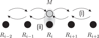
Figure 1: Basic operations with a marker atom on a quantum register: (i) forward and backward transport steps. (ii) local interaction with register qubits.

The role of the $M$ qubits in our scheme is twofold. On one hand they will allow us to address single register atoms without the need for addressing single lattice sites, i.e. they act as a “marker” for a certain register atom. On the other hand they act as information carrier performing effective entangling operations between physically distant register qubits. In this case they act as a “messenger” transporting quantum information. However, to simplify language, in the following we will denote the $M$ qubits always as marker qubits or marker atoms.

The interaction we apply depends on the logical state of both of the involved qubits, i.e. it enables us to perform two-qubit gates like a controlled-phase or a swap gate between the marker and the register atom. This in turn, combined with forward and backward transport operations (i), allows to construct sequences of operations that enact two-qubit gates between arbitrary register qubits. This works as follows (see Fig. 2):

• the state of qubit $R_{i}$ is first swapped onto the marker $M$;

• the marker is transported to location $j$, where a two-qubit gate is performed between $M$ and $R_{j}$;

• the marker is transported back to location $i$ and its state is swapped back onto $R_{i}$.

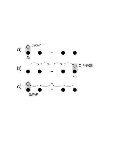
Figure 2: Realizing an entangling operation between distant atoms based on the elementary steps described in Fig. 1: a) swapping the first qubit onto the marker atom; b) transporting the marker atom unto the second qubit and local interaction; c) transport back to the first qubit and inverse swap.

At the end of the process, the marker qubit recovers its initial state, while the net effect is that a gate operation has been performed between register qubits $R_{i}$ and $R_{j}$. Beside logical operations, this allows for the creation of distant entangled (e.g., EPR) pairs that can be subsequently used for teleportation between different quantum memory locations, for state purification in error correcting protocols and for scalable probabilistic gates Duan et al. (2004).

II.2 Implementation of the concept with atoms in periodic trapping potentials

In the following we want to briefly outline how the above general concept can be implemented. A detailed description can be found in Sec. III-V. As described above the two key ingredients of our scheme are (i) the transport of marker atoms and (ii) the application of a strong local interaction. We concentrate in this work on an implementation with neutral atoms stored in a two-component optical superlattice. However, our scheme may be transferred to other systems, including atom chips Folman et al. (2000). We consider single atoms stored in the ground state of separate wells which we model as a 1D periodic potential (see Sec. III.1), with a simple filling pattern of one register atom $R_{i}$ every second lattice site. The ground states of the remaining sites may (or may not) be occupied by marker atoms, which can be of the same species as the register atoms, and the tunnel coupling between neighboring sites is assumed to be negligible, so that marker atoms do not interact with register atoms unless the potential is modified. The quantum information is stored in two appropriate internal states $|0\rangle,\,|1\rangle$ of the atoms (which will be specified in Sec. IV).

As described in Section III, the transport of the marker atoms (i) is realized by globally changing the external lattice control parameters which allows for creating a periodic array of double-well structures with different well depths. In this way the marker atom can be transferred from its initial site into the first excited state of one of the neighboring wells, while the register atom located there (as well as any other register atom in the lattice) remains in its trap ground state. From here the marker can be transported further to the ground state of the next site (which is not occupied by an atom) or back again to its initial position. By repeating these transport steps the marker atoms can be transported to an arbitary lattice site. This scheme avoids there being two permanently interacting atoms at any lattice site.

Due to the fact that the lattice parameters are changed globally, all marker atoms undergo the same, parallel movement. Thus, when more ground-state marker atoms are introduced at different sites, a certain lattice transformation will transport all of them in the same way. By suitably choosing the pattern of marker atoms, multi-qubit operations can be carried out in parallel or with pre-defined patterns (an example is encoding and syndrome extraction for error correction).

When a marker and a register atom are at the same site we realize the coupling (ii) of Fig. 1 by making use of the strong molecular interaction between the marker and the register atom, which can be controlled by an external magnetic field giving rise to a Feshbach resonance Pethick and Smith (2002). The physics behind this mechanism, as well as the gate operations, will be detailed in Secs. IV and V, respectively. Of course, this sort of interaction can be employed in any neutral-atom quantum computation proposal. In this paper, we will outline its general features, and we will focus on its specific use in the context of marker-atom quantum computing.

The principle of the single qubit gate is the following. The marker atom is transported to the register atom we want to address. Then the molecular interaction is “switched on” via an external magnetic or optical field, i.e. we perform a Feshbach ramp which leads to a level splitting of the atomic states. Clearly this splitting is only present at the site with two atoms. With appropriately detuned external lasers we can then perform arbitrary single qubit rotations

$$|0\rangle\longrightarrow \cos(\alpha)|1\rangle-\mathrm{i}\sin(\alpha)\mathrm{e}^{\mathrm{i}\varphi}|0\rangle$$

$$|1\rangle\longrightarrow -\mathrm{i}\sin(\alpha)|1\rangle+\cos(\alpha)\mathrm{e}^{\mathrm{i}\varphi}|0\rangle$$ (1)

where the angle $\alpha$ is given by the interaction time with the lasers (and their intensities) and the phase $\phi$ is determined by the dynamics of the Feshbach ramp. The lasers have not to be focused down to the lattice constant. The spatial width is merely limited by the distance to the next marker atom (except if we want to perform the same rotation there).

The principle of two qubit gates is already shown in Fig. 2 where in step $b)$ we either perform a swap operation between register and marker atom, $|\epsilon_{1}\epsilon_{2}\rangle\rightarrow|\epsilon_{2}\epsilon_{1}\rangle$, or a phase gate, $|\epsilon_{1}\epsilon_{2}\rangle\rightarrow\exp[\mathrm{i}\varphi(1-\epsilon_{1})(1-\epsilon_{2})]|\epsilon_{1}\epsilon_{2}\rangle$ where $\epsilon_{1,2}\in\{0,1\}$. As we will describe in Sec. V, the phase gate as well as the swap gate are again based on the tunable molecular interaction between two atoms at one lattice site. In the first case the phase is acquired by a Feshbach ramp which affects only the state $|00\rangle$ while in the case of the swap gate we need, similar as in the case of the single qubit rotation, an additional laser field which couples resonantly the state which is shifted by the molecular interaction and the states $|01\rangle$ and $|10\rangle$. The laser will again affect only the sites where two atoms are present thus again it does not have to be focused.

Beside relaxing addressability constraints, our scheme bears several other advantages: for instance, it does not require a state-dependent lattice Jaksch et al. (1999). As described in Sec. I that method has a couple of disadvantages and, furthermore, the realization and stabilization of such potentials poses a major experimental challenge. In our scheme the quantum register logical state never gets entangled with the atomic motion, eliminating a major source of decoherence. Even collisional phases, acquired by the marker atom while being transported over occupied lattice sites, can be made state-insensitive by an appropriate choice of the atomic hyperfine states (a typical example being Rb, for which the singlet and the triplet scattering lengths coincide), thus contributing only a global phase to the evolution of the whole register.

III Atom transport in time dependent superlattices

The transport scheme we describe in this section makes use of a time dependent optical superlattice configuration which can be far-offresonant from the relevant optical transition to avoid spontaneous emission and is not specialized to specific atomic species. The atom transport is independent of the considered internal states and allows for using the $m=0$ states of different hyperfine manifolds, i.e. states of a “clock transition” which are not affected by external magnetic fields.

In the following we will describe the laser configuration which is necessary to realize the superlattice and detail the transport of single atoms in the periodic potential by changing the intensities and phases of the lasers. We will furthermore discuss optimization methods.

III.1 Realization of the superlattice

For the realization of the superlattice potential we propose using a configuration of four intersecting lasers like it was used in Peil et al. (2003). The setup is shown in Fig. 3.

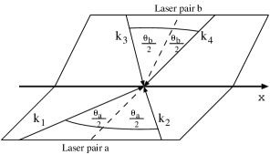
Figure 3: Laser setup. The plane containing the wavevectors $\vec{k}_{1,2}$ of a laser pair $a$ intersects the plane containing the wavevectors $\vec{k}_{3,4}$ of a laser pair $b$ at the $x$-axis. The planes can have a finite angle between them. The angle between the lasers in each of the pairs are $\theta_{a}$ and $\theta_{b}$, respectively (see also Peil et al. (2003)).

Two pairs of laser beams intersect with an angle $\theta_{a}$ and $\theta_{b}$, respectively The lasers of frequency $\omega_{a}$ (pair a) and $\omega_{b}$ (pair b) interact with atoms which are considered as two level systems with transition frequency $\omega_{0}$. In an interaction picture, the Hamiltonian for the internal degrees of freedom of an atom can then be written as

$$H=H_{0}+\hbar\Delta_{a}\sigma_{+}\sigma_{-}-\frac{1}{2}\Big{[} \sigma_{+}\vec{d}\left(\vec{E}_{a}(\vec{r})+\vec{E}_{b}(\vec{r})\mathrm{e}^{\mathrm{i}\delta t}\right)$$

$$+ \sigma_{-}{\vec{d}}^{*}\left({\vec{E}}_{a}^{\dagger}(\vec{r})+{\vec{E}_{b}}^{\dagger}(\vec{r})\mathrm{e}^{-\mathrm{i}\delta t}\right)\Big{]}$$ (2)

where $H_{0}={\vec{p}}^{\;2}/2m$ is the kinetic energy operator. Furthermore we introduced $\Delta_{a,b}=\omega_{0}-\omega_{a,b}$, $\delta=\omega_{a}-\omega_{b}$, the atomic dipole moment $\vec{d}$ and the electric fields

$$\vec{E}_{a}(\vec{r}) = \sum_{j=1,2}\mathcal{E}_{j}\vec{\varepsilon}_{j}\mathrm{e}^{\mathrm{i}(\vec{k}_{j}\vec{r}+\phi_{j})},$$ (3)

$$\vec{E}_{b}(\vec{r}) = \sum_{j=3,4}\mathcal{E}_{j}\vec{\varepsilon}_{j}\mathrm{e}^{\mathrm{i}(\vec{k}_{j}\vec{r}+\phi_{j})},$$ (4)

where $\vec{\varepsilon}_{j}$ are the normalized polarization vectors, $\mathcal{E}_{j}$ the field amplitudes and the wavevectors have the magnitude $k_{a}\equiv|\vec{k}_{1}|=|\vec{k}_{2}|=\omega_{a}/c$, $k_{b}\equiv|\vec{k}_{3}|=|\vec{k}_{4}|=\omega_{b}/c$.
The laser pairs are assumed to be far off detuned from atomic resonance and from each other so we can adiabatically eliminate the upper atomic level and obtain an effective Hamiltonian in position representation

$$H_{\text{eff}}=-\frac{\hbar^{2}}{2m}{\vec{\nabla}}^{2}-\left(\frac{|\vec{d}\vec{E}_{a}(\vec{r})|^{2}}{4\hbar\Delta_{a}}+\frac{|\vec{d}\vec{E}_{b}(\vec{r})|^{2}}{4\hbar\Delta_{b}}\right).$$ (5)

According to the geometry of the laser setup the second term of Eq. (5) can be written as

$$U(x) =-\Bigg{[}\frac{1}{4\hbar\Delta_{a}}\sum_{j=1,2}|\vec{d}\vec{\varepsilon}_{j}|^{2}\mathcal{E}_{j}^{2}+\frac{1}{4\hbar\Delta_{b}}\sum_{j=3,4}|\vec{d}\vec{\varepsilon}_{j}|^{2}\mathcal{E}_{j}^{2}$$

$$+\frac{(\vec{d}\vec{\varepsilon}_{1})({\vec{d}}^{*}\vec{\varepsilon}_{2})\mathcal{E}_{1}\mathcal{E}_{2}}{4\hbar\Delta_{a}}\cos\big{(}2k_{a}x\sin(\theta_{a}/2)+\phi_{1}-\phi_{2}\big{)}$$

$$+\frac{(\vec{d}\vec{\varepsilon}_{3})({\vec{d}}^{*}\vec{\varepsilon}_{4})\mathcal{E}_{3}\mathcal{E}_{4}}{4\hbar\Delta_{b}}\cos\big{(}2k_{b}x\sin(\theta_{b}/2)+\phi_{3}-\phi_{4}\big{)}\Bigg{]}$$ (6)

$$\equiv U_{0}+U_{1}\cos\big{(}2k_{a}x\sin(\theta_{a}/2)+\phi_{1}-\phi_{2}\big{)}$$

$$\quad+U_{2}\cos\big{(}2k_{b}x\sin(\theta_{b}/2)+\phi_{3}-\phi_{4}\big{)},$$ (7)

where $U_{0}$ is merely a constant. In Sec. III.2 we will choose it according to Eq. (10). If we set $\phi_{1}=\phi_{2}$, $\phi\equiv\phi_{4}-\phi_{3}$, $\theta_{a}=\pi$ (counterpropagating lasers) and

$$\theta_{b}=2\arcsin\left(\frac{k_{a}}{2k_{b}}\right)\approx 2\arcsin\left(\frac{1}{2}\right)=\frac{\pi}{3},$$ (8)

the potential is of the type

$$U(x)=U_{0}+U_{1}\cos(2\kappa x)+U_{2}\cos(\kappa x-\phi).$$ (9)

The potential (9) leads to a particle confinement along the $x$ axis. We will assume in the following the confinement in the transverse directions $y$ and $z$ to be much stronger than along the $x$-direction so that we have effectively a one dimensional system.

III.2 Single atom transport

The transport of an atom through the lattice is achieved by varying the amplitudes $U_{i}(t)$ and the relative phase $\phi(t)$ of the two lattice components, which is done by changing the intensities and phases of the lasers-see Eq. (6). The potential (9) becomes then time dependent: $U(x)\rightarrow U(x,t)$.

Figure 4: Potential $U(x,t)$ at two different times and $V=100\,E_{r}$ (with recoil energy $E_{r}=\hbar^{2}\kappa^{2}/2m$). At $t_{0}=0$ $u_{1}(0)=u_{2}(0)=0$ (dashed line) while at $t_{1}>0$ we set $u_{1}(t_{1})=0.5,\,u_{2}(t_{2})=0.2$ and $\sigma=1,\,l=0$ (solid line). In the latter case the difference between the minima is approximately $20\,E_{r}$ and the height of every second barrier is reduced by approximately $50\%$.

For the description of the transport process it is useful to rewrite the potential (9) depending on two parameters $u_{1}(t)$ and $u_{2}(t)$:

$$U_{0}(t) = \frac{V}{4}[2-u_{1}(t)+u_{2}(t)],$$ (10)

$$U_{1}(t) = \frac{V}{4}[2-u_{1}(t)-u_{2}(t)],$$ (11)

$$U_{2}(t) = \frac{V}{2}\sqrt{u_{1}^{2}(t)+u_{2}(t)^{2}},$$ (12)

$$\phi(t) = \sigma\arctan{[u_{2}(t)/u_{1}(t)+l\pi]}.$$ (13)

At time $t=0$ we set $U_{2}(t)=0$, i.e. $u_{1}(0)=u_{2}(0)=0$ and thus we simply have a cosine-potential of depth $V$ and periodicity $a_{0}=\pi/\kappa$. However, in general the periodicity of the lattice is $a_{1}=2\pi/\kappa$ and the shape of the optical potential can be designed in the following way:

The parameter $u_{1}(t)$ controls approximately the height $V[1-u_{1}(t)]$ of every second barrier depending on the parameter $l\in\{0,1\}$: If $l=0$ the height of every “odd” barrier is changed while in case of $l=1$ the height of every “even” barrier is changed, i.e. in the first case barriers with maxima at $x=(2j+1)\pi/\kappa$ and in the latter case barriers with maxima at $x=2j\pi/\kappa$ are modified for $U_{2}=0$ and $j\in\mathbb{Z}$. By changing $u_{1}(t)$ we can thus create a specific periodic array of double well potentials. The parameter $u_{2}(t)$ controls additionally the difference of the minima $Vu_{2}(t)$ of such a double well potential, while $\sigma\in\{\pm 1\}$ determines if the left ($\sigma=1$) or right ($\sigma=-1$) well is raised.

An example is shown in Fig. 4 for $l=0,\,\sigma=1$ and two different values for $u_{1}$ and $u_{2}$. The potential $U(x,t)$ is given in units of the recoil energy $E_{r}=\hbar^{2}\kappa^{2}/2m$ where $m$ is the atomic mass appearing in the time dependent Schrödinger equation

$$\mathrm{i}\hbar\frac{d}{dt}\psi(x,t)=-\frac{\hbar^{2}}{2m}\frac{d^{2}}{dx^{2}}\psi(x,t)+U(x,t)\psi(x,t)$$ (14)

which has to be solved for the study of single atom transport.

Figure 5: Illustration of steps (i)-(iv) of the transport process as described in the text. Shown are also the square of the absolute value of the single particle wavefunctions of the atom which is transported (i.e. the “marker atom”), $|\psi^{M}(x)|^{2}$ (solid lines), and of the register atom which is supposed to remain at its lattice site, $|\psi^{R}(x)|^{2}$ (dashed lines). The example shown requires $\sigma=1$ and $l=0$.

The elementary steps of the atom transport are done by tunnelling in the double well potentials. An example is shown in Fig. 5 for $\sigma=1$, $l=0$ and $V=100\,E_{r}$:

At the initial time $t=0$, where $u_{1}(0)=u_{2}(0)=0$, we consider two neighboring wells, with one atom in the motional ground state of the left well (Fig. 5a). The probability densities $|\psi^{M}(x,t)|^{2}$ of the atom are indicated by the solid lines in this figure. The superscript $M$ indicates the wavefunction of the atom to be transported, i.e. the wavefunction of the “marker atom” as introduced in Sec II. Also shown in this figure by the dashed lines are the probability densities of the “register atom” $|\psi^{R}(x,t)|^{2}$, initially located in the ground state of the right well in this example and which is supposed to remain at its lattice site during the transport. Our goal in the process described here is to transfer the left atom into the first excited state of the right well without affecting the other one. This can be accomplished by changing the parameters $u_{1,2}(t)$ according to the following steps, which are illustrated in Fig. 5:

• Between the times $t=0$ and $t=t_{1}$ we raise very rapidly the minimum of the left well, such that its ground state crosses in energy the right well’s first excited state.

• In the time interval $[t_{1},t_{2}]$ we lower the central barrier down to a point where the atom can tunnel from left to right while at the same time we start to lower the left well.

• In the time interval $[t_{2},t_{3}]$ the barrier is raised up again while we continue to lower back the left well.

• During the time interval $[t_{3},t_{4}]$ we restore the initial potential shape.

By doing steps (ii) and (iii) adiabatically the atom stays in the second excited state of the double well potential which is at $t_{1}$ the ground state of the left well and at $t_{3}$ the first excited state of the right well. Thus the atom is transported from left to right.

An effective transport procedure requires appropriate “pulse functions” $u_{1}(t)$ and $u_{2}(t)$ while the direction of the transport is governed by the parameters $\sigma,l$. Let us assume for simplicity that the marker atom is located initially at a site $\kappa x_{j}=(2j+1/2)\pi,\,j\in\mathbb{Z}$. Then the process shown in Fig. 5 requires $\sigma=1$ and $l=0$ while for a further movement to the motional ground state on the right we have to set $\sigma=-1$ and $l=1$ and to perform the same pulse functions backwards in time. For moving an atom from the ground state to the first excited state of the left neighboring well we have to set $\sigma=-1$ and $l=1$ and to apply the forward pulse functions. In this case a further movement to the left ground state requires $\sigma=1$ and $l=0$ and the backward pulse function. Note that the abrupt changes of the phase $\phi$ take place while $U_{2}$ is zero, i.e. when the corresponding lasers are completely blocked off from the atoms. Every transport of an atom across the lattice can be divided into these four elementary processes. Since the pulse sequence is in all cases the same (except for time reversal) we can focus in the following on the example shown in Fig. 5.

The feasibility of our quantum computing scheme depends on the time scale on which quantum operations can be performed. Clearly the latter is directly connected to the speed of the transport process. In this respect steps (i) and (iv) can be performed over much shorter times than step (ii) and (iii), which are limited for example by the energy difference to the other motional states. In order to examine adiabatic transport during step (ii) and (iii) it is thus necessary to study the instantaneous eigenenergies of an atom during the transport process in dependence on the parameters we can control, i.e. the pulse functions $u_{1,2}(t)$.

Since $U(x,t)$ is periodic, we can calculate the instantaneous eigenenergies and eigenfunctions of the single particle Hamiltonian by introducing Bloch functions $\psi_{k}^{(n)}(x)=e^{\mathrm{i}kx}u_{k}^{(n)}(x)$ with Bloch vector $k$ and band index $n$. In Fourier space the stationary Schrödinger equation takes the form

$$\frac{\hbar^{2}}{2m}(q-k)^{2}\tilde{u}_{k}^{(n)}(q,t) +\sum_{q^{\prime}}\tilde{U}(q-q^{\prime},t)\tilde{u}_{k}^{(n)}(q,t)$$

$$=E_{k}^{(n)}(t)\tilde{u}_{k}^{(n)}(q,t),$$ (15)

where

$$\tilde{u}_{k}^{(n)}(q,t)=\frac{1}{a_{i}}\int_{0}^{a_{i}}dx\,\mathrm{e}^{\mathrm{i}qx}u_{k}^{(n)}(x,t),$$

$$u_{k}(x,t)=\sum_{q}\mathrm{e}^{-\mathrm{i}qx}\tilde{u}_{k}(q,t),\quad q=\frac{2n\pi}{a_{i}},\,n\in\mathbb{Z}$$ (16)

and

$$\tilde{U}(q,t)=U_{0}(t)\delta_{q,0}+ \frac{U_{1}(t)}{2}(\delta_{2\kappa,q}+\delta_{2\kappa,-q})$$

$$+ \frac{U_{2}(t)}{2}(\mathrm{e}^{\mathrm{i}\phi(t)}\delta_{\kappa,q}+\mathrm{e}^{-\mathrm{i}\phi(t)}\delta_{\kappa,-q}).$$ (17)

where $a_{i}$ with $i=0,1$ are the lattice constants, i.e. $a_{0}=\pi/\kappa$ if $U_{2}=0$ and $a_{1}=2\pi/\kappa$ if $U_{2}\neq 0$. By assuming periodic boundary conditions the Bloch vector $k$ gets quantized, i.e. $k=2n\pi/Ma_{0},\,n=-M/2,\ldots,M/2$ where $M$ is the number of lattice sites. Given the functions $u_{k}(x)$ we can furthermore construct Wannier functions which are localized at lattice sites $x_{i}$,

$$w^{(n)}(x-x_{i})=\frac{1}{\sqrt{M}}\sum_{k}\mathrm{e}^{\mathrm{i}k(x-x_{i})}u_{k}^{(n)}(x).$$ (18)

These functions are needed for example as initial states for solving the time dependent Schrödinger equation (14). Since in our considerations the lowest bands are always practically flat, i.e. the Bloch states for a given band are approximately degenerate, the Wannier functions are also in good approximation eigenstates of the Hamiltonian and thus dispersion of the wave packet during the time evolution is negligible.

Figure 6: Band structures for two different values of $u_{1},u_{2}$ and $V=100E_{r},\,\sigma=1,\,l=0$. (a) Initial values of the lattice parameters ($u_{1}(0)=u_{2}(0)=0$). (b) Band structure during the transport process ($u_{1}=0.99,\,u_{2}=0.13$). The two figures correspond to the situations shown in Figs. 5a and 5c.

Equation (III.2) is a linear system of equations which can be solved numerically after truncating $q$ at sufficiently high values. The instantaneous eigenenergies $E_{k}^{(n)}(t)$ gained in this way are very important to find an adiabatic passage for the atom transport. An example for the band structure is shown in Fig. 6. As can be seen from this figure, $V$ is sufficiently large to be in a tight binding regime, i.e. the lower bands are flat and there is no tunnelling between different wells.

For an efficient adiabatic transport the pulse functions have now to be chosen such that the corresponding energies $E_{k}^{(n)}(t)$ behave in an appropriate way during the transport steps (ii) and (iii), i.e. one should for example avoid level crossings of the initial energy with the energies of other states. An example is shown in Fig. 7a.

As already mentioned the Bloch states in the lowest bands are almost degenerate so we can restrict ourselves to a an arbitrary value of $k$, e.g. $k=0$. The upper solid line in this figure corresponds to the “path” of the atom to be transported initially located in the left well while the lower solid line indicates the path of the atom located in the right well. The initial depth of the potential wells is $V=100\,E_{r}$ leading to a “trap frequency” in a single well of about $20\,\omega_{r}$ ($\omega_{r}\equiv E_{r}/\hbar$ is the recoil frequency). Keeping the height of the barrier constant we raise the minimum of the left well such that the ground state energy of the left well crosses the first excited state energy of the right well [step (i)]. Then we proceed according to steps (ii) and (iii). By reducing the height of the central barriers the trap frequency decreases and by adjusting appropriately the pulse functions we avoid that the solid lines cross the dashed lines. After time $t_{3}$ the original potential shape is restored [step (iv)]. The pulse functions $u_{1,2}(t)$ used for this example and the corresponding time dependent physical relevant parameters $U_{1,2}(t),\,\phi(t)$ are shown in Fig. 7b and Figs. 7cd, respectively.

Figure 7: Adiabatic atom transfer between lattice sites: (a) Instantaneous eigenenergies $E^{(n)}_{k=0}(t)$. The upper solid line corresponds to the motional energy of the atom to be transported and the lower solid line corresponds to the register atom initially in the right well (cf. Fig. 5). (b) Corresponding control parameters $u_{1,2}$. (c) Amplitudes of the lattice components. (d) Phase difference between lattice components. The time axis is given in units of the recoil frequency $\omega_{r}\equiv E_{r}/\hbar$. The time interval $[t_{1},t_{3}]$ is not of the same scale as $[0,t_{1}],[t_{3},t_{4}]$.

The fidelities of the processes, given by

$$F^{A}=\left|\int dx\,{\psi^{A}}^{*}(x,T)\psi^{A}_{\text{fin}}(x)\right|^{2},$$ (19)

are numerically calculated by solving the time dependent single particle Schrödinger equation in position representation (14) by using the Crank-Nicholson scheme Press et al. (1992) where as initial state $\psi^{A}_{\text{ini}}$ and final state $\psi^{A}_{\text{fin}}$ we choose Wannier functions (18) which are located in the corresponding wells. The superscript $A\in\{M,R\}$ indicates again the wavefunction of the atom to be transported (marker atom) and the atom which is supposed to stay located at its well (register atom).

In case of the example of Fig. 7 we get $F^{M}=99.91\%$ for propagating the marker atom wavefunction and $F^{R}=99.98\%$ for propagating the register atom wavefunction from $t_{1}$ to $t_{3}$ in a time $T=t_{3}-t_{1}=20/\omega_{r}$. In the case of Rubidium ($\omega_{r}=2\pi\times 3.8\,\mathrm{kHz}$) this would correspond to a time $T=0.8\,\mathrm{ms}$ and for sodium ($\omega_{r}=2\pi\times 25\,\mathrm{kHz}$) we would have $T=130\,\mu\mathrm{s}$. For the optical superlattice described in Peil et al. (2003) a laser power of $P=3\,\mathrm{mW}$ was sufficient to create a maximal potential depth of $2U_{i}<60E_{R}$ for $\sideset{{}^{87}}{}{\operatorname{\mathrm{Rb}}}$. Keeping the ratio of laser intensity and detuning constant we have $U_{i}\sim\sqrt{P}$. For a potential depth of roughly $U_{i}<50E_{R}$ which is required in the above example (see Fig. 7c) we can estimate the required maximal laser power to be merely $P\approx 8-9\,\mathrm{mW}$.

III.3 Pulse optimization

If we relax the constraint of adiabatic transport during step (ii) and (iii) the process described in the previous subsection can be significantly accelerated. In this case the pulse sequences have to be engineered in a certain way which can be done by using quantum optimal control techniques as detailed, e.g., in Peirce et al. (1988); Borzi et al. (2002); Sklarz and Tannor (2002). Thereby the evolution of a quantum system governed by a set of control parameters (in our case these are the functions $u_{1,2}(t)$) is tailored to reach a pre-determined target state $\psi_{\text{fin}}$ with optimized fidelity within a specific time $T$. For notational convenience we will denote in the following the time $t=t_{1}$ as $t=0$ and $t=t_{3}$ as $t=T$.

The basic idea is to minimize the infidelity of the process with the constraint that the Schrödinger equation has to be fulfilled. This amounts to find the stationary point of a functional, leading to a set of equations for the wavefunction and auxiliary states $\chi^{A}$ which are introduced as Lagrange multipliers. In our case this functional takes the form

$$\mathcal{L}(\psi^{M},\psi^{R},\dot{\psi}^{M},\dot{\psi}^{R},\chi^{M},\chi^{R},u_{1},u_{2})=$$

$$\qquad\sum_{A\in\{M,R\}}\Bigg{[}1-\left|\int dx\,\psi^{A}_{\mathrm{fin}}(x){\psi^{A}}^{*}(x,T)\right|^{2}$$

$$\qquad+2\mathrm{Re}\Bigg{(}\int_{0}^{T}dt\int dx\,\chi^{A}(x,t)\big{(}\dot{\psi}^{A}(x,t)$$

$$\qquad\qquad\qquad+\frac{\mathrm{i}}{\hbar}H(u_{1}(t),u_{2}(t))\psi^{A}(x,t)\big{)}^{*}\Bigg{)}\Bigg{]},$$ (20)

with

$$H(u_{1}(t),u_{2}(t))=-\frac{\hbar^{2}}{2m}\frac{d^{2}}{dx^{2}}+U(x,u_{1}(t),u_{2}(t)),$$ (21)

where the last term in Eq. (21) is the potential (9), which depends on the control parameters. As can be seen from Eq. (20) we are looking for a minimum of the sum of the infidelities of the process for the marker atom and the register atom. Setting the derivatives with respect to the arguments of $\mathcal{L}$ equal to zero leads to the following set of equations,

$$\mathrm{i}\hbar\dot{\psi}^{A}(x,t)=H(u_{1}(t),u_{2}(t))\psi^{A}(x,t),\quad A\in\{R,M\},$$ (22)

$$\mathrm{i}\hbar\dot{\chi}^{A}(x,t)=H(u_{1}(t),u_{2}(t))\chi^{A}(x,t),\quad A\in\{R,M\}$$ (23)

with conditions

$$\psi^{A}(x,0)=\psi^{A}_{\text{ini}}(x),$$ (24)

$$\chi^{A}(x,T)\equiv\psi_{\text{fin}}^{A}(x)\int dx\,\psi_{\text{fin}}^{A}(x){\psi^{A}}^{*}(x,T),$$ (25)

and

$$0=-2\mathrm{Im}\sum_{A\in\{M,R\}}K_{j}^{A}(u_{1}(t),u_{2}(t)),\quad j=1,2$$ (26)

with

$$K_{j}^{A}(u_{1} (t),u_{2}(t))\equiv$$

$$\int dx\,\psi^{A}(x,t)\frac{\partial U(x,u_{1}(t),u_{2}(t))}{\hbar\partial u_{j}(t)}{\chi^{A}}^{*}(x,t).$$ (27)

These equations are the basis of the optimal control algorithm which minimizes $\mathcal{L}$ with respect to $u_{j}$. Thereby we solve Eq. (22) and (23) numerically by introducing a discretized time axis with time step $\Delta t$ and by using the Crank-Nicholson scheme. For the sake of completeness we briefly describe the algorithm we use here. The following procedure, called immediate feedback control, is guaranteed to give a fidelity improvement at each iteration Sola et al. (1998).

The Schrödinger equations (22) are integrated from $t=0$ to $t=T$ leading to $\psi^{A}(x,T)$ with an initial guess for the control parameters $u_{1,2}^{(0)}(t)$. At this point an iterative algorithm starts during which the controls $u_{1,2}^{(n)}(t)$ are updated.

Let us assume that we are in the $n$-th iteration. Taking the controls $u_{1,2}^{(n)}(t)$, Eqs. (23) have to be solved backwards in time, i.e. from $t=T$ to $t=0$, with “end values” (25) which can be interpreted as the part of $\psi^{A}(x,T)$ that has reached the objective. Given the solutions $\chi^{A}(x,0)$ the functions $\chi^{A}(x,t)$ and $\psi^{A}(x,t)$ (with initial conditions (24)) are now again evolved forward in time while the control parameters are updated during each time step according to

$$u_{j}^{(n+1)}(t)=u_{j}^{(n)}(t)+\frac{2}{\lambda(t)}\text{Im}\sum_{A\in\{M,R\}}K_{j}^{A}(u_{1}^{(n)}(t),u^{(n)}_{2}(t)).$$

During the forward evolution $\chi(x,t+\Delta t)$ is calculated using the controls $u_{1,2}^{(n)}(t)$ while $\psi(x,t+\Delta t)$ is evolved according to $u_{1,2}^{(n+1)}(t)$. The weight $\lambda(t)$ is used to enforce fixed initial and final conditions on the control pulses. Given these solutions we go on with the next iteration.

The results of such a calculation after $135$ iterations are shown in Fig. 8 which corresponds to the situation of Fig. 5: Fig. 8a shows the control parameters for transferring the marker atom to the first excited state of its right neighboring site while keeping the register atom at its initial location. Fig. 8bc shows the corresponding physical parameters. As starting values $u^{(0)}_{1,2}(t)$ we took the pulses of the adiabatic example (see Fig. 7). The use of the optimized pulses leads to a reduction of the transport time down to $T_{3}=5\hbar/E_{R}$, which corresponds to $200\,\mu\mathrm{s}$ for rubidium and to $32\,\mu\mathrm{s}$ for sodium with a fidelity of $F^{M}=F^{R}=99.99\%$.

Figure 8: Non-adiabatic atom transfer between lattice sites: (a) Control parameters $u_{1,2}$. (b) Corresponding amplitudes of the lattice components. (c) Phase difference between lattice components. The time axis is given in units of the recoil frequency $\omega_{r}\equiv E_{r}/\hbar$. The time interval $[t_{1},t_{3}]$ is not of the same scale as $[0,t_{1}],[t_{3},t_{4}]$.

IV Coherent resonant collisions in a trap

The coupling scheme we are proposing can be implemented either in dipole-force potentials, like optical lattices Jessen and Deutsch (1996), or in static electromagnetic traps, like atom chips Folman et al. (2000). Performing gate operations as described in Sec. IV requires a strong molecular interaction between register atom and marker atom. Atoms can be coupled to molecular states either by means of Feshbach resonances Pethick and Smith (2002) or through Raman photoassociation laser pulses Weiner et al. (1999). For the sake of concreteness, we focus here on Feshbach resonances in optical lattices – however, all of our arguments can be adapted, e.g., to Raman photoassociation on atom chips. We consider ⁸⁷Rb atoms trapped in a two-component optical lattice (see, e.g., Peil et al. (2003)).

IV.1 Feshbach resonances in confined geometry

A schematic picture of the Born-Oppenheimer potential describing their interaction in the relative coordinate $r$ is shown in Fig. 9.

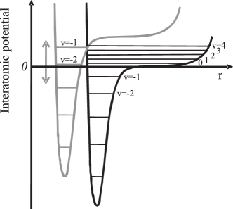
Figure 9: Interaction of two atoms in an external trap. The two curves schematically describe the Born-Oppenheimer potential for two scattering channels around a Feshbach resonance.

Negative values of the excitation number $v$ label bound molecular eigenstates of the dimer system, while positive $v$ values denote unbound trapped two-atom states. Such a potential exists for each collision channel $|\beta\rangle$, corresponding to the relative-motion and hyperfine angular momentum quantum numbers of the two colliding atoms. Feshbach resonances occur when a bound state $|n_{\beta}\rangle$ ($v=-2$ in the example shown) crosses the dissociation threshold for a state having the same quantum numbers Pethick and Smith (2002) while changing an external magnetic field $B$. Close to resonance, the scattering length varies as

$$A_{\beta}(B)=A_{bg}\left(1-\frac{\Delta_{\beta}}{B-B_{\beta}}\right),$$ (29)

where $A_{bg}$ is a non resonant background scattering length, $B_{\beta}$ is the resonant magnetic field, and $\Delta_{\beta}$ is the width of the resonance. The resonance energy varies almost linearly with the field

$$\varepsilon_{\beta}(B)=s_{\beta}(B-B_{\beta}),$$ (30)

with a slope $s_{\beta}$. We are interested in the dynamics of such a system in a confined geometry. Following Mies et al. (2000), we shall model it by the effective Hamiltonian

$$H_{\beta}=\varepsilon_{\beta}(B)|n_{\beta}\rangle\langle n_{\beta}|+\sum_{v}(v\hbar\nu|v\rangle\langle v|+V_{v}^{\beta}|v\rangle\langle n_{\beta}|+{\rm h.c.}),$$ (31)

where the $|v\rangle$’s are the trapped relative-motion atomic eigenstates of an isotropic harmonic oscillator trap having frequency $\nu$. The couplings to the resonance are

$$V_{v}^{\beta}=2\hbar\nu\sqrt{\sqrt{4v+3}\;a_{bg}\delta_{\beta}/\pi}$$ (32)

with $a_{bg}\equiv A_{bg}\sqrt{m\nu/\hbar}$, $\delta_{\beta}\equiv\Delta_{\beta}s_{\beta}/(\hbar\nu)$. In a different geometry, for instance in an elongated trap characterized by a ratio $\gamma$ between the ground level spacings in the transverse and in the longitudinal potential, the couplings can be calculated by projection on the corresponding eigenstates (see Appendix A). Accurate values for the resonance parameters $\Delta_{\beta}$ and $B_{\beta}$, as well as for $A_{bg}$, are now available from both theoretical calculations and recent measurements Marte et al. (2002).

The possibility of controlling the resonance energy via an external magnetic field, as described by Eq. (30), provides a straightforward way to steer the interaction between the atoms. Not only can the scattering length be varied over a significant range – the atoms can also be adiabatically coupled into a molecular state. An example of this sort of process is shown in Fig. 10. Here, the eigenvalues of the interacting Hamiltonian are shown for a six-level model including the five lowest unbound trap states plus the resonant state. The latter is ramped across threshold by applying an external magnetic field having a linear dependence on time. Both the so-called “diabatic” energies (i.e. those obtained by neglecting the couplings to the resonance) and the adiabatic ones (i.e. the actual eigenvalues of the full coupled Hamiltonian) are plotted against time for a certain ramp rate. The important point to notice is that the ground state of the relative motion is adiabatically connected to the resonant state. Therefore, if the atoms are prepared in their relative-motion ground state and the resonance state is ramped across threshold from above, the atoms are transferred into the bound state, whose energy depends on the magnetic field - and the process is actually reversible. This mechanism has been used for the creation of molecules in ultracold gases Wynar et al. (2002); Xu et al. (2003); Donley et al. (2002); Regal et al. (2003); Herbig et al. (2003); Cubizolles et al. (2003); Dürr et al. (2004), and is very relevant in the present context of quantum information processing due to its inherent state-dependent nature. Indeed, the coupling to a specific resonant state $|n_{\beta}\rangle$ is only effective for a particular entrance channel $|\beta\rangle$, while in general all other combinations of atomic hyperfine states (that is, of logical qubit states in our case) will be unaffected by the resonance. Thus the resonance-induced energy shift will cause a two-particle phase to appear only for that particular two-qubit computational basis state. We will see in the next Section how to use this effect in order to achieve a desired C-phase gate.

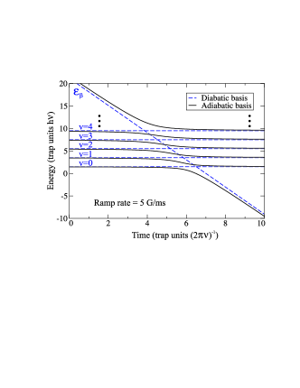
Figure 10: Adiabatic (solid) and diabatic (dashed) energies of a 6-level expansion (molecular resonance level plus 5 trap levels of an isotropic 100 kHz trap) with a linear ramp of magnetic field with slope 5 G/ms. The adiabatic energy levels show a set of avoided crossings. We use the Feshbach resonance level near 100 mT. The coupling matrix element $V_{0}$is 0.884 $h\nu$ for this trap.

IV.2 Choosing qubit logical states

We will identify our qubit logical states with the clock-transition states

$$\left|0\right\rangle\equiv\left|F=1,m_{F}=0\right\rangle,\quad\left|1\right\rangle\equiv\left|F=2,m_{F}=0\right\rangle$$ (33)

and the auxiliary state as

$$|x\rangle\equiv|F=1,m_{F}=1\rangle.$$ (34)

The main advantage of this choice is that the qubit states are not sensitive to the magnetic field, and hence not subject to decoherence due to its fluctuations.

The level scheme for a single atom is shown in Fig. 11.

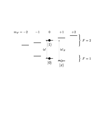
Figure 11: Internal level scheme for a single atom: qubit and auxiliary states.

When we consider two atoms, the relevant level scheme is described by Fig. 12, if they occupy their relative-motion ground state. Appendix B shows that this is indeed the case for two bosons stored in the ground and first axial excited state of a cigar-shaped harmonic trap.

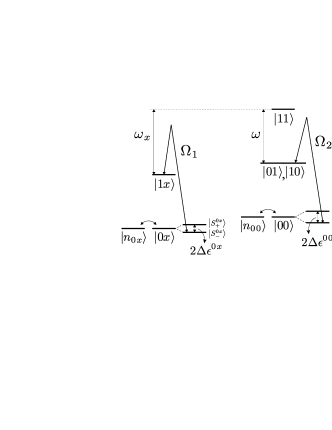
Figure 12: Internal level scheme for two coupled atoms: levels involved in single- (left) and in two-qubit operations (right). The Raman transitions $\Omega_{1}$ ($\Omega_{2}$) used for single- (two-)qubit operations are shown.

In Fig. 12 the resonant levels $|n_{\beta}\rangle$ are also shown, which are used to induce energy shifts for the purpose of gate operation as described in the next Section. Indeed, in a confined geometry, the coupling to such molecular states can induce dressing of the trapped eigenstates with a half-splitting $\Delta\epsilon^{\beta}$ – controllable, by varying the external field, up to a maximum value equal on resonance to the interaction strength $V^{\beta}$ –, as shown in Fig. 12 for the collisional channels $|\beta\rangle=|00\rangle,|0x\rangle$.

Our calculation with a realistic molecular interaction potential yields, among others, two resonances at $B_{0x}=386$ G and $B_{00}=407$ G, having widths $\Delta_{0x}=5.7$ mG and $\Delta_{00}=16$ mG, as shown in Fig. 13. These will be employed in the following to effect logical gate operations.

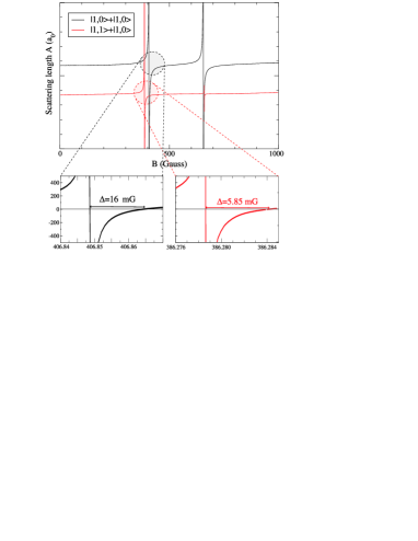
Figure 13: Dependence of the scattering length of ⁸⁷Rb on the external magnetic field for collisions in channels $|00\rangle$ and $|0x\rangle$.

V Quantum operations

Let us now examine in detail how to use the features described above in order to perform quantum computation in our system. Preparing all atoms in an initial state by optical pumping requires no single-qubit addressing and can be performed with standard techniques. As the next step, according with the above discussion, performing a specific algorithm will require a certain pattern of marker atoms. These can be prepared either in a periodic fashion, by means of a superlattice tuned to the appropriate transition, or in an ad hoc lattice region, spatially separated from the one where computation has to take place, to be subsequently loaded into the latter via the transport mechanism detailed above.

V.1 Single-qubit gates

In the single-qubit case, the relevant resonance field is $B_{0x}$, while the lasers couple $|1x\rangle$ with the lower dressed state connected to $|0x\rangle$ with an effective Rabi frequency $\Omega_{1}$ as in Fig. 12.b. The process is resonant only if the marker atom in state $|x\rangle$ is present. In this way, specific sites where the single-qubit operation takes place can be selected even if the addressing laser cannot resolve them spatially from neighboring sites. Moreover, the two-atoms state remains always factorized, whence possible magnetic field fluctuations, affecting the state $|x\rangle$ (unlike $|0\rangle$ and $|1\rangle$) will yield only a global phase. In a rotating frame the Hamiltonian which describes this system takes the form

$$H= \delta|1x\rangle\langle 1x|+\varepsilon_{0x}(B)|M\rangle\langle M|$$

$$+ V_{0}^{0x}\big{(}|0x\rangle\langle M|+|M\rangle\langle 0x|\big{)}+\frac{\Omega_{1}}{2}\big{(}|0x\rangle\langle 1x|+|1x\rangle\langle 0x|\big{)}$$ (35)

where $\delta$ is the Raman detuning of two co-propagating Raman lasers, $V_{0}^{0x}$ is the coupling between the molecular state $|M\rangle$ and the dissociated state $|0x\rangle$ and $\varepsilon_{0x}(B)$ is the energy of the molecular state (we set the energy of the $|0x\rangle$ state to zero). At the beginning of the operation the lasers are switched off (i.e. $\Omega_{1}=0$) and the external magnetic field is adiabatically tuned to the Feshbach resonance, i.e. $\varepsilon_{0x}(B)\rightarrow\varepsilon_{0x}(B_{0x})=0$. This leads to a splitting of the two particle state $|0x\rangle$ in two new eigenstates,

$$|S_{\pm}^{0x}\rangle=\frac{1}{\sqrt{2}}\big{(}|0x\rangle\pm|M\rangle\big{)}.\\$$ (36)

These states are indicated in the left hand side of Fig. 11 (here we have $\Delta\epsilon^{0x}=V^{0x}_{0}$ since we are on resonance). For finite laser power, in this basis the Hamiltonian takes the form

$$H= \delta|1x\rangle\langle 1x|+V_{0}^{0x}(|S_{+}^{0x}\rangle\langle S_{+}^{0x}|-|S_{-}^{0x}\rangle\langle S_{-}^{0x}|)$$

$$+\frac{\Omega_{R}}{2\sqrt{2}}\Big{[}\big{(}|S_{+}^{0x}\rangle+|S_{-}^{0x}\rangle\big{)}\langle 1x|+|1x\rangle\big{(}\langle S_{+}^{0x}|+\langle S_{-}^{0x}|\big{)}\Big{]}.$$ (37)

The Raman detuning is set to $\delta=-V_{0}^{0x}$ and if $\Omega_{0}/V_{0}^{0x}\ll 1$ we can project out the state $|S_{+}^{0x}\rangle$. This yields the two level Hamiltonian

$$H= -V_{0}^{0x}\big{(}|1x\rangle\langle 1x|+|S_{-}^{0x}\rangle\langle S_{-}^{0x}|\big{)}$$

$$+\frac{\Omega_{1}}{2\sqrt{2}}\Big{(}|S_{-}^{0x}\rangle\langle 1x|+|1x\rangle\langle S_{-}^{0x}|\Big{)}$$ (38)

i.e. if we finally tune the magnetic field out of the Feshbach resonance again we get the transformation

$$|0x\rangle\rightarrow \cos(\Omega_{1}/2\sqrt{2}t)|1x\rangle-\mathrm{i}\sin(\Omega_{1}/2\sqrt{2}t)\mathrm{e}^{\mathrm{i}\varphi}|0x\rangle,$$ (39)

$$|1x\rangle\rightarrow -\mathrm{i}\sin(\Omega_{1}/2\sqrt{2}t)|1x\rangle+\cos(\Omega_{1}/2\sqrt{2}t)\mathrm{e}^{\mathrm{i}\varphi}|0x\rangle.$$ (40)

In this expression we included a phase $\varphi$ which is the (adjustable) phase accumulated during the adiabatic ramping process of the magnetic field.

V.2 Two-qubit gates

In the two-qubit case, we take the marker atom to be in a state of the logical subspace spanned by $|0\rangle$ and $|1\rangle$. This time, the field is ramped across $B_{00}$, and the Raman lasers couple for a time $\tau$ – with Rabi frequency $\Omega_{2}$ – the lower dressed state to the degenerate two-atom levels $|01\rangle$ and $|10\rangle$ (Fig. 12.c). In a rotating frame the Hamiltonian can be written as

$$H= \delta\big{(}|01\rangle\langle 01|+|10\rangle\langle 10|\big{)}+2\delta|11\rangle\langle 11|$$

$$+\varepsilon_{00}(B)|M\rangle\langle M|+V_{0}^{00}\big{(}|M\rangle\langle 00|+|00\rangle\langle M|\big{)}$$

$$+\frac{\Omega_{2}}{2}\big{(}|00\rangle\langle 01|+|00\rangle\langle 10|+|11\rangle\langle 01|+|11\rangle\langle 10|+\text{h.c.}\big{)}.$$ (41)

The notations are the same as in Eq. (35). We perform now the same procedure as in the case of the single qubit rotation, i.e. we tune adiabatically the magnetic field to the Feshbach resonance, i.e. $\varepsilon_{00}(B_{00})=0$ while $\Omega_{2}=0$. The Hamiltonian with diagonalized molecular part reads

$$H= \delta\big{(}|01\rangle\langle 01|+|10\rangle\langle 10|\big{)}+2\delta|11\rangle\langle 11|$$

$$+V_{0}^{00}\big{(}|S_{+}^{00}\rangle\langle S_{+}^{00}|-|S_{-}^{00}\rangle\langle S_{-}^{00}|\big{)}$$

$$+\frac{\Omega_{R}}{2\sqrt{2}}\Big{[}\big{(}|S_{+}^{00}\rangle+|S_{-}^{00}\rangle\big{)}\langle 01|+\big{(}|S_{+}^{00}\rangle+|S_{-}^{00}\rangle\big{)}\langle 10|$$

$$+|11\rangle\langle 01|+|11\rangle\langle 10|+\text{h.c.}\Big{]},$$ (42)

where

$$|S_{\pm}^{00}\rangle=\frac{1}{\sqrt{2}}\big{(}|00\rangle\pm|M\rangle\big{)},\\$$ (43)

These states are shown on the right hand side of Fig. 11 (now we have $\Delta\epsilon^{00}=V^{00}_{0}$). Taking the Raman detuning to be $\delta=-V_{0}^{00}$ amounts to the fact that (if $\Omega_{2}/V_{0}^{00}\ll 1$) the states $|11\rangle$ and $|S_{+}^{00}\rangle$ are effectively decoupled from the remaining three states. Projecting out the uncoupled states the effective Hamiltonian for the remaining three level system then takes the form

$$H= -V_{0}^{00}\big{(}|S_{-}^{00}\rangle\langle S_{-}^{00}|+|01\rangle\langle 01|+|10\rangle\langle 10|\big{)}$$

$$+\frac{\Omega_{0}}{2\sqrt{2}}\big{(}|S_{-}^{00}\rangle\langle 01|+|S_{-}^{00}\rangle\langle 10|+|01\rangle\langle S_{-}^{00}|+|10\rangle\langle S_{-}^{00}|\big{)}.$$ (44)

If we introduce the vector notation $|\psi\rangle\leftrightarrow\big{(}\langle S_{-}^{00}|\psi\rangle,\,\langle 01|\psi\rangle,\,\langle 10|\psi\rangle\big{)}^{T}$ and disregard global phases the time evolution operator of this system can be written as

$$U(t)= \frac{1}{2}\begin{pmatrix}2c(t)&-\mathrm{i}s(t)&-\mathrm{i}s(t)\\ -\mathrm{i}s(t)&c(t)+1&c(t)-1\\ -\mathrm{i}s(t)&c(t)-1&c(t)+1\end{pmatrix}$$ (45)

with $c(t)=\cos(\Omega_{2}t/2)$ and $s(t)=\cos(\Omega_{2}t/2)$. If we apply a Raman pulse of duration $\tau=2(2n+1)\pi/\Omega_{2}$ and finally tune the magnetic field out of the Feshbach resonance again, we get the following truth table for the operation:

$$|00\rangle\longrightarrow-\mathrm{e}^{\mathrm{i}\varphi}|00\rangle,$$

$$|01\rangle\longrightarrow-|01\rangle,$$

$$|10\rangle\longrightarrow-|10\rangle,$$

$$|11\rangle\longrightarrow\mathrm{e}^{\mathrm{i}V_{0}^{00}\tau}|11\rangle,$$ (46)

where we included again the phase $\varphi$ now accumulated by state $|00\rangle$ during the ramping process due to the interaction energy shift, whose value can be adjusted by controlling the magnetic field. For $\varphi=2\pi$ and $V_{0}^{00}\tau=(2m+1)\pi$ – which imposes a commensurability condition $\Omega_{2}/V_{0}^{00}=2(2n+1)/(2m+1)$ between the Rabi frequency and the Feshbach energy shift –, a swap operation is performed. Besides being an essential ingredient for entangling gates between distant atoms as detailed in Sec. II, such a swap operation can greatly help in the task of non-destructive qubit readout. To this aim, the quantum state of an atom to be read out at the end of a computation could be simply swapped onto a marker atom to be subsequently transported to a different lattice region where measurement can take place without physically disturbing the register atoms, which can be later re-used for logical operations.

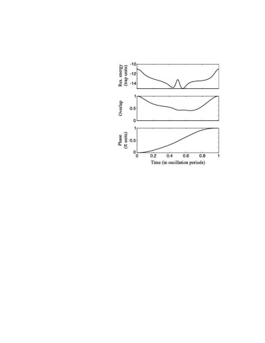
Figure 14: Two-qubit (C-phase) gate operation: resonance energy $\varepsilon_{00}$ (top; off-resonant before and after gate operation), overlap between evolved and initial state (center), accumulated phase (bottom).

On the other hand, if no Raman lasers are present and $\varphi=\pi$, a C-phase gate between register and marker atom is obtained. A two qubit gate between distant register atoms can be realized as described in Sec. II. Note that laser addressing of single qubits is never required throughout the procedure.

The magnetic ramping process can be even performed non-adiabatically, provided that all population is finally returned to the trapped atomic ground state. This can be accomplished via a quantum optimal control technique in analogy with the above discussion for the transport process. The control parameter in this case is the resonance energy $\varepsilon_{00}$, which can be adjusted by varying the external magnetic field. Care has to be taken in optimizing not only the absolute value of the overlap of the final state onto the goal state, but also its phase $\varphi$. Fig. 14 shows the optimization results for a 100 kHz trap with a ratio of $\nu_{\perp}/\nu=10$ between the trap frequencies $\nu_{\perp}$ in $y,z$-direction and $\nu$ in $x$-direction. The final infidelity is about $2\times 10^{-5}$ in this case.

VI Conclusions

When it comes to using neutral atoms for the purpose of quantum information processing, besides the well-known general criteria formulated by D. DiVincenzo DiVincenzo (2000), the fulfillment of various practical requirements, specific to atomic implementations, can make a difference on the road to experimental realization. For example laser addressing of single qubits, though being theoretically trivial, is limited by diffraction, imposing a lower bound on the actual spacing between qubits. Furthermore performing gate operations in state-dependent potentials creates entanglement between internal and external degrees of freedom, which in turn is prone to decoherence, as random fields typically affect differently the two logical states. The same is true for internal-state entanglement, if the qubit states are chosen with different Landé factor and, unless the latter vanishes for both states, they will be sensitive to magnetic-field fluctuations.

In this paper, we introduced the concept of “marking” qubits via molecular interactions which allows for relaxing a number of these constraints for neutral-atom quantum computing. We have presented a scheme that enables quantum gates and information transport in a quantum register, even though requiring neither single-site addressing by externally applied fields nor state-dependent external potential. Moreover, qubit states with the same (even vanishing) Landé factor can be employed; and the overall speed can be of the order of the inverse atomic trapping frequency. We have shown how this scheme can be implemented in two-component optical lattices, whereby the mechanism used to mark atoms is the molecular interaction responsible for Feshbach resonances, which are currently a subject of intense experimental research in the field of cold atoms, where molecule formation via control of Feshbach resonances has been recently achieved Xu et al. (2003); Donley et al. (2002); Regal et al. (2003); Herbig et al. (2003); Cubizolles et al. (2003); Dürr et al. (2004). In other words, our proposal relies on techniques that are presently being developed, and represents therefore a feasible candidate for the implementation of quantum information processing with neutral atoms in optical lattices.

Finally, the analysis presented here is limited to one-dimensional systems, basically with a single marker atom. Further conceptual development is possible, for instance in exploring the interplay between several marker atoms on the same lattice, or the extended flexibility given for instance by higher-dimensional geometries; this will be the subject of future investigations.

Appendix A Dynamics in a cigar-shaped trap

The normalized eigenfunctions of a 3D harmonic oscillator in spherical coordinates are

$$\Phi_{n\ell m_{\ell}}^{\mathrm{sph}}(r,\theta,\phi) = \sqrt{\frac{2\alpha^{2\ell+3}\Gamma(n+\ell+3/2)}{n!\Gamma(\ell+3/2)^{2}}}r^{\ell}e^{-\alpha^{2}r^{2}/2}\times$$ (47)

$${}_{1}F_{1}(-n,\ell+3/2,\alpha^{2}r^{2})Y_{\ell}^{m_{\ell}}(\theta,\phi)$$

where $\alpha=\sqrt{m\nu/\hbar}$, $\Gamma(n)$ is the Euler Gamma function, ${}_{1}F_{1}(a,b,z)$ is the Kummer confluent hypergeometric function, and $Y_{\ell}^{m_{\ell}}(\theta,\phi)$ are the spherical harmonics. The normalized eigenfunctions in cylindrical coordinates (we assume the same frequency $\nu$ in the longitudinal direction, and a transverse frequency $\nu_{\perp}$ a factor $\gamma$ higher) are:

$$\Phi_{n\ell m_{\ell}}^{\mathrm{cyl}}(\rho,\phi,z) = \frac{(\alpha\rho)^{|m_{\ell}|}e^{im_{\ell}\phi-(\alpha^{2}\gamma\rho^{2}+\alpha^{2}z^{2})/2}}{\sqrt{2^{n}\ell!(\sqrt{\pi}/\alpha)^{3}}}\times$$

$$H_{n}(\alpha z)\,_{1}F_{1}(-\ell,\left|m_{\ell}\right|+1,\gamma\alpha^{2}\rho^{2})/$$

$$\sqrt{\sum_{i,j=0}^{\ell}\frac{(-\ell)_{i}(-\ell)_{j}\Gamma(|m_{\ell}|+i+j+1)}{i!j!(m_{\ell}+1)_{i}(m_{\ell}+1)_{j}\gamma^{|m_{\ell}|+1}}}$$

where $H_{n}(x)$ are the Hermite polynomials, and $(a)_{i}=\Gamma(a+i)/\Gamma(a)$ is the Pochhammer symbol. We are interested in $s$-wave scattering processes, so we restrict our analysis to the eigenstates with $\ell=m_{\ell}=0$ and obtain

$$\langle\Phi_{2v+1,0,0}^{\mathrm{cyl}}|\Phi_{w,0,0}^{\mathrm{sph}}\rangle\! \!=\! \!0;$$ (49)

$$\langle\Phi_{2v,0,0}^{\mathrm{cyl}}|\Phi_{w,0,0}^{\mathrm{sph}}\rangle\! \!=\! \!(-2)^{-v}\sqrt{\gamma 2^{3-w}(2v)!w!(2w+1)!!}$$

$$\!\times\! \!\sum_{i=0}^{w}\sum_{j=0}^{v}\frac{(-4)^{i+j}(2i+2j+1)!!}{(2i+1)!(2j+1)!}\qquad$$

$$\!\times\! \!\frac{{}_{1}F_{1}\left(j+\frac{1}{2},i+j+\frac{3}{2},j+\frac{3}{2},\frac{\gamma-1}{\gamma+1}\right)}{\left(v-j\right)!(w-i)!(\gamma+1)^{i+j+3/2}}$$

The coupling matrix elements in a cigar-shaped trap with anisotropy factor $\gamma\neq 1$ are computed as

$$V_{v}^{\beta}(\gamma)=\sum_{w}\langle\Phi_{v00}^{\mathrm{cyl}}|\Phi_{w00}^{\mathrm{sph}}\rangle V_{w}^{\beta}(\gamma=1),$$ (51)

where the spherical matrix elements $V_{w}(\gamma=1)$ are given by Eq. (32).

Appendix B Conditional level shift in a quasi-1D trap

Let us consider the three-dimensional state $\left|\Psi_{S,m_{S}}\right\rangle$ of two spin-1/2 bosons in a harmonic trap. In the $\hat{x}$ direction, one particle is in the trap ground state $\left|\psi_{0}\right\rangle$, and the other in the first excited state $\left|\psi_{1}\right\rangle$. The transverse state is the ground state $\left|\psi_{\perp}\right\rangle$ for both particles. $X$ and $x$ are the center-of-mass and relative coordinate. Denoting the $i^{\rm th}$ particle’s state by $|\cdot\rangle_{i}$, the symmetrized states can be written as

$$\left|\Psi_{0,0}\right\rangle =\frac{\left|1\right\rangle_{1}\left|0\right\rangle_{2}-\left|0\right\rangle_{1}\left|1\right\rangle_{2}}{\sqrt{2}}\frac{|\psi_{1}\rangle_{1}|\psi_{0}\rangle_{2}-|\psi_{0}\rangle_{1}|\psi_{1}\rangle_{2}}{\sqrt{2}}$$

$$=\frac{\left|1\right\rangle_{1}\left|0\right\rangle_{2}-\left|0\right\rangle_{1}\left|1\right\rangle_{2}}{\sqrt{2}}|\psi_{0}\rangle_{X}|\psi_{1}\rangle_{x};$$ (52)

$$\left|\Psi_{1,-1}\right\rangle =\left|0\right\rangle_{1}\left|0\right\rangle_{2}\frac{|\psi_{1}\rangle_{1}|\psi_{0}\rangle_{2}+|\psi_{0}\rangle_{1}|\psi_{1}\rangle_{2}}{\sqrt{2}}$$

$$=\left|0\right\rangle_{1}\left|0\right\rangle_{2}|\psi_{1}\rangle_{X}|\psi_{0}\rangle_{x};$$ (53)

$$\left|\Psi_{1,0}\right\rangle =\frac{\left|1\right\rangle_{1}\left|0\right\rangle_{2}+\left|0\right\rangle_{1}\left|1\right\rangle_{2}}{\sqrt{2}}\frac{|\psi_{1}\rangle_{1}|\psi_{0}\rangle_{2}+|\psi_{0}\rangle_{1}|\psi_{1}\rangle_{2}}{\sqrt{2}}$$

$$=\frac{\left|1\right\rangle_{1}\left|0\right\rangle_{2}+\left|0\right\rangle_{1}\left|1\right\rangle_{2}}{\sqrt{2}}|\psi_{1}\rangle_{X}|\psi_{0}\rangle_{x};$$ (54)

$$\left|\Psi_{1,1}\right\rangle =\left|1\right\rangle_{1}\left|1\right\rangle_{2}\frac{|\psi_{1}\rangle_{1}|\psi_{0}\rangle_{2}+|\psi_{0}\rangle_{1}|\psi_{1}\rangle_{2}}{\sqrt{2}}$$

$$=\left|1\right\rangle_{1}\left|1\right\rangle_{2}|\psi_{1}\rangle_{X}|\psi_{0}\rangle_{x}.$$ (55)

When we apply a static external magnetic field corresponding to the Feshbach resonance for the $|00\rangle$ channel, the interaction only affects the state $\left|\Psi_{1,-1}\right\rangle$, dressing it with a splitting $2V_{0}^{00}(\gamma)$ that can easily be of the order of $\hbar\nu$ assuming a ratio $\nu_{\perp}/\nu=10$ of the trap frequancy $\nu_{\perp}$ in $y,z$-direction and $\nu$ in $x$-direction. This means that the state $\left|0\right\rangle_{1}\left|0\right\rangle_{2}$ can be discriminated spectroscopically, allowing for different kinds of gate operation as described in the text.

References

- Cirac and Zoller (2004) J. I. Cirac and P. Zoller, Phys. Today 57, 38 (2004).
- Greiner et al. (2002) M. Greiner, O. Mandel, T. Esslinger, T. W. Hänsch, and I. Bloch, Nature 415, 39 (2002).
- Charron et al. (2002) E. Charron, E. Tiesinga, F. Mies, and C. Williams, Phys. Rev. Lett. 88, 077901 (2002).
- Tian and Zoller (2003) L. Tian and P. Zoller, Phys. Rev. A 68, 042321 (2003).
- Pachos and Knight (2003) J. K. Pachos and P. L. Knight, Phys. Rev. Lett. 91, 107902 (2003).
- Dorner et al. (2003) U. Dorner, P. Fedichev, D. Jaksch, and P. Zoller, Phys. Rev. Lett. 91, 073601 (2003).
- Rabl et al. (2003) P. Rabl, A. J. Daley, P. O. Fedichev, J. I. Cirac, and P. Zoller, Phys. Rev. Lett. 91, 110403 (2003).
- Mompart et al. (2003) J. Mompart, K. Eckert, W. Ertmer, G. Birkl, and M. Lewenstein, Phys. Rev. Lett. 90, 147901 (2003).
- Eckert et al. (2002) K. Eckert, J. Mompart, X. X. Yi, J. Schliemann, D. Bruß, G. Birkl, and M. Lewenstein, Phys. Rev. A 66, 042317 (2002).
- Lukin et al. (2001) M. D. Lukin, M. Fleischhauer, R. Côté, L. M. Duan, D. Jaksch, J. I. Cirac, and P. Zoller, Phys. Rev. Lett. 87, 037901 (2001).
- Andersson and Stenholm (2001) E. Andersson and S. Stenholm, Opt. Commun. 188, 141 (2001).
- García-Ripoll and Cirac (2003) J. J. García-Ripoll and J. I. Cirac, Phys. Rev. Lett. 90, 127902 (2003).
- Brennen et al. (2000) G. K. Brennen, I. H. Deutsch, and P. S. Jessen, Phys. Rev. A 61, 062309 (2000).
- Brennen et al. (1999) G. K. Brennen, C. M. Caves, P. S. Jessen, and I. H. Deutsch, Phys. Rev. Lett. 82, 1060 (1999).
- Schlosser et al. (2001) N. Schlosser, G. Reymond, I. Protsenko, and P. Grangier, Nature 411, 1024 (2001).
- Dumke et al. (2002) R. Dumke, T. Müther, M. Volk, W. Ertmer, and G. Birkl, Phys. Rev. Lett. 89, 220402 (2002).
- Dür et al. (1999) W. Dür, H. Briegel, J. I. Cirac, and P. Zoller, Phys. Rev. A 59, 169 (1999).
- Folman et al. (2002) R. Folman, P. Krueger, J. Schmiedmayer, J. Denschlag, and C. Henkel, Adv. At. Mol. Opt. Phys. 48, 263 (2002).
- Farooqi et al. (2003) S. M. Farooqi, D. Tong, S. Krishnan, J. Stanojevic, Y. P. Zhang, J. R. Ensher, A. S. Estrin, C. Boisseau, R. Côté, E. E. Eyler, et al., Phys. Rev. Lett. 91, 183002 (2003).
- Duan et al. (2004) L.-M. Duan, B. B. Blinov, D. L. Moehring, and C. Monroe (2004), eprint quant-ph/0401020.
- Folman et al. (2000) R. Folman, P. Krüger, D. Cassettari, B. Hessmo, T. Maier, and J. Schmiedmayer, Phys. Rev. Lett. 84, 4749 (2000).
- Pethick and Smith (2002) C. J. Pethick and H. Smith, Bose-Einstein Condensation in Dilute Gases (Cambridge University Press, Cambridge, 2002).
- Jaksch et al. (1999) D. Jaksch, H.-J. Briegel, J. I. Cirac, C. W. Gardiner, and P. Zoller, Phys. Rev. Lett. 82, 1975 (1999).
- Peil et al. (2003) S. Peil, J. V. Porto, B. Laburthe Tolra, J. M. Obrecht, B. E. King, M. Subbotin, S. L. Rolston, and W. D. Phillips, Phys. Rev. A 67, R051603 (2003).
- Press et al. (1992) W. H. Press, S. A. Teukolsky, W. T. Vetterling, and B. P. Flannery, Numerical Recipes in C (Cambridge University Press, Cambridge, 1992), 2nd ed.
- Peirce et al. (1988) A. P. Peirce, M. A. Dahleh, and H. Rabitz, Phys. Rev. A 37, 4950 (1988).
- Borzi et al. (2002) A. Borzi, G. Stadler, and U. Hohenester, Phys. Rev. A 66, 053811 (2002).
- Sklarz and Tannor (2002) S. Sklarz and D. Tannor, Phys. Rev. A 66, 53619 (2002).
- Sola et al. (1998) I. R. Sola, J. Santamaria, and D. J. Tannor, J. Phys. Chem. 102, 4301 (1998).
- Jessen and Deutsch (1996) P. S. Jessen and I. H. Deutsch, Adv. At. Mol. Opt. Phys 37, 95 (1996).
- Weiner et al. (1999) J. Weiner, V. S. Bagnato, S. Zilio, and P. S. Julienne, Rev. Mod. Phys. 71, 1 (1999).
- Mies et al. (2000) F. H. Mies, E. Tiesinga, and P. S. Julienne, Phys. Rev. A 61, 022721 (2000).
- Marte et al. (2002) A. Marte, T. Volz, J. Schuster, S. Dürr, G. Rempe, E. G. M. van Kempen, and B. J. Verhaar, Phys. Rev. Lett. 89, 283202 (2002).
- Wynar et al. (2002) R. Wynar, R. S. Freeland, D. J. Han, C. Ryu, and D. J. Heinzen, Science 287, 1016 (2002).
- Xu et al. (2003) K. Xu, T. Mukaiyama, J. R. Abo-Shaeer, J. K. Chin, D. E. Miller, and W. Ketterle, Phys. Rev. Lett. 91, 210402 (2003).
- Donley et al. (2002) E. Donley, N. R. Claussen, S. T. Thompson, and C. E. Wieman, Nature 417, 529 (2002).
- Regal et al. (2003) C. A. Regal, C. Ticknor, J. L. Bohn, and D. S. Jin, 424, 47 (2003).
- Herbig et al. (2003) J. Herbig, T. Kraemer, M. Mark, T. Weber, C. Chin, H. C. Nägerl, and R. Grimm, Science 301, 1510 (2003).
- Cubizolles et al. (2003) J. Cubizolles, T. Bourdel, S. Kokkelmans, G. V. Shlyapnikov, and C. Salomon, Phys. Rev. Lett. 91, 240401 (2003).
- Dürr et al. (2004) S. Dürr, T. Volz, A. Marte, and G. Rempe, Phys. Rev. Lett. 92, 020406 (2004).
- DiVincenzo (2000) D. P. DiVincenzo, Fort. Phys. 48, 771 (2000).