Complete conditions for entanglement transfer

Abstract

We investigate the conditions to entangle two qubits interacting with local environments driven by a continuous-variable correlated field. We find the conditions to transfer the entanglement from the driving field to the qubits both in dynamical and steady-state cases. We see how the quantum correlations initially present in the driving field play a critical role in the entanglement-transfer process. The system we treat is general enough to be adapted to different physical setups.

Quantum networks of remote local processors, which are interconnected by quantum and classical channels, have been investigated to effectively perform quantum computation gottesman and quantum communication  duan . A quantum repeater has also been proposed for error-tolerant long-haul quantum communication briegel . These schemes require a reliable channel to entangle remote nodes in order to use in later steps of protocols. The usage of a light field to implement a quantum channel is a natural choice because of its handiness in generating and propagating entanglement furusawa . However, we have witnessed that all optical network is technically extremely challenging KLM . On the other hand, static qubits such as the hyperfine structure of atoms are easily accessible and manipulative by means of external excitations. Therefore, it may be an optimal strategy to use an optical quantum channel to bring quantum correlation to two remote sites of static qubits, where the entanglement is subsequently utilized for quantum information processing. It is, thus, evident that the study of entanglement transfer from an optical field of a continuous-variable (CV) system to a static qubit system has a primary importance.

Recently, such entanglement generation on the pair of remote qubits has been studied through the indirect interaction via projective measurement plenio , two-mode squeezed driving field sp ; kraus and a non-Markovian braun and a Markovian environments benatti . Although these schemes successfully demonstrate the situation for entanglement generation on remote qubits, the complete physical requirements for the possible creation of entanglement are unknown. In this paper, we investigate the sufficient and necessary conditions to induce entanglement on two remote qubits, by means of their respective linear interactions with a two-mode driving field.

From its definition, entanglement between any two systems cannot be created by local unitary operations alone. Thus, when the driving field is separable, there is no way to generate the entanglement between the two qubits. The natural least constraint of the entanglement of the qubits is the entanglement of the state for the quantum channel. However it is not clear if entanglement of the driving field can always be transferred to the static qubits. We study both the dynamical and the steady-state cases.

Master equation - We analyze the dynamics of two remote qubit systems sketched in Fig. 1.

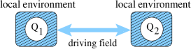
Figure 1: Scheme of the system considered. Two individual qubits ($Q_{1},\,Q_{2}$), each interacting with their local environment, are driven by a quantum correlated field.

Each qubit of its ground $\left|g\right\rangle_{i}$ and excited $\left|e\right\rangle_{i}$ states ($i=1,\,2$) interacts with its own local environment of a single-mode bosonic system. We will refer to local environments by modes $a$ and $b$. Static qubits such as ions, atoms or quantum dot devices are isolated from uncontrollable real-world environment. A coupling of the static qubit with the driving field is thus assumed to be through their small local environments which isolate the qubits from the uncontrollable environment. We model each qubit-bosonic interaction by a resonant Hamiltonian ($\hbar=1$), $\hat{H}_{a1}+\hat{H}_{b2}$, where $\hat{H}_{a1}=\Omega_{a1}\left(\hat{\sigma}^{+}_{1}\hat{a}+\hat{a}^{{\dagger}}\hat{\sigma}^{-}_{1}\right)$ (analogously for $\hat{H}_{b2}$). Here, $\hat{a}$ and $\hat{a}^{\dagger}$ are standard bosonic operators, $\hat{\sigma}^{+}_{1}=(\hat{\sigma}^{-}_{1})^{{\dagger}}=\left|e\right\rangle_{1}\!\left\langle g\right|$ and $\Omega_{a1}$ is the Rabi frequency. The dynamics of the two qubits is guided by an external broadband two-mode driving field (bandwidth $\Delta\omega_{ext}$). The coupling between modes $a,\,b$ and the external driving field is written as $\hat{V}(t)=\sum_{j}\kappa_{j}\left(\hat{a}\hat{\cal G}_{aj}^{\dagger}(t){e}^{i\omega_{a}t}+\hat{a}^{\dagger}\hat{\cal G}_{aj}(t){e}^{-i\omega_{a}t}+a\leftrightarrow{b}\right)$, where $\hat{\cal G}_{aj}(t)=\hat{a}_{j}\mbox{e}^{i\omega_{j}t}$ with $\hat{a}_{j}$ the annihilation operator of the driving field in frequency $\omega_{j}$, is coupled at rate $\kappa_{j}$ to mode $a$. Here, $\omega_{a,b}$ are the frequencies of modes $a$ and $b$. In the weak coupling limit $\kappa_{j}\ll\omega_{a,b},\Delta\omega_{ext}$ ($\forall{j}$), we use second-order perturbation theory and the first Born-Markov approximation. The evolution of modes $a,\,b$ can, then, be described by a Liouvillian super-operator ${\hat{\cal L}}$ involving only the second-order moments of quadrature variables for the driving field  wallsmilburn in its carrier frequency $\omega_{0}$, which is set to be resonant to the qubit transition, i.e., $\omega_{0}=\omega_{a}=\omega_{b}$. The coupling rate in this frequency is denoted by $\kappa$. The dynamics of the total system can, thus, be described by the master equation $\partial_{t}\rho=-i[\hat{H}_{a1}+\hat{H}_{b2},\rho]+{\cal\hat{L}}\rho=\left(\hat{\cal L}_{o}+\hat{\cal L}\right)\rho$, with $\rho$ the density matrix of the qubits+local environments system.

In order to characterize the master equation, we need to consider only the second-order quadrature moments matrix for the driving field which can be written by a matrix ${\bf M}$ . The matrix elements are $M_{\alpha\beta}=\langle\{\hat{x}_{\alpha},\hat{x}_{\beta}\}\rangle$ with quadrature operator vector $\hat{\bf x}=(\hat{q}_{1},\hat{p}_{1},\hat{q}_{2},\hat{p}_{2})$. Without changing the entanglement structure of the driving field, a very general real matrix $\bf M$ can be transformed into the simple form by local unitary operations simon (no matter the driving field being Gaussian or non-Gaussian)

$${\bf M}=\begin{pmatrix}{\bf n}&{\bf c}\\ {\bf c}&{\bf m}\end{pmatrix}$$ (1)

with ${\bf n}=n\mbox{$1{\bf l}$}_{2}$, ${\bf m}=m\mbox{$1{\bf l}$}_{2}$ ($n,m\geq{0}$) that describe the local properties of each mode and ${\bf c}=diag[c_{1},\,c_{2}]$ that accounts for the inter-mode correlations.

We are interested in the qubit evolution so to eliminate the modes $a,\,b$. This can be done using an adiabatic elimination procedure valid in the weak-coupling regime $\kappa\gg\Omega_{a1},\Omega_{b2}$. In this case, the dynamics of the modes interacting with the driving field is much faster than their interaction with the qubits. The qubits see modes $a$ and $b$ in a steady state $\rho_{ss}$ not affected by the qubit-modes dynamics. The adiabatic elimination proceeds by defining a projection operator as ${\cal P}\rho=\rho_{ss}\otimes{Tr}_{ab}(\rho)=\rho_{ss}\otimes\rho_{12}$. Here $\rho_{12}$ is the density matrix of the qubits. Using the property ${\cal P}\hat{\cal L}_{o}{\cal P}\rho=0$, the reduced master equation takes the form $\partial_{t}\rho_{12}={Tr}_{ab}\left\{\hat{\cal L}_{o}\int^{\infty}_{0}e^{\hat{\cal L}t}\hat{\cal L}_{o}\left(\rho_{ss}\otimes\rho_{12}\right)dt\right\}$. It is straightforward to find that the dynamics of the qubits is fully described by the effective Liouvillian

$$\hat{\cal L}_{e}\rho_{12}=\sum^{4}_{\alpha,\beta=1}D_{\alpha\beta}\left(\hat{{\cal O}}_{\alpha}\rho_{12}\hat{{\cal O}}_{\beta}-\frac{1}{2}\left\{\hat{{\cal O}}_{\beta}\hat{{\cal O}}_{\alpha},\rho_{12}\right\}\right),$$ (2)

with $\hat{{\cal O}}_{\alpha}=\sigma_{\alpha}\otimes\mbox{$1{\bf l}$}$ for $\alpha=1,2$ and $\hat{{\cal O}}_{\alpha}=\mbox{$1{\bf l}$}\otimes\sigma_{\alpha-2}$ for $\alpha=3,4$, $\sigma_{1,2}$ the $x$ and $y$ Pauli operators. The Kossakowski matrix is ${\bf D}=\{\{{\bf A},{\bf C}\},\{{\bf C}^{\dagger},{\bf B}\}\}$, where ${\bf A}={\bf A}^{\dagger}$, ${\bf B}={\bf B}^{\dagger}$ and ${\bf C}$ are $2\times 2$ matrices benatti . For the driving field with its second-order moments as in Eq. (1), we get

$${\bf A}=\frac{\gamma_{1}}{4}\begin{pmatrix}n&i\\ -i&n\\ \end{pmatrix}\,{\bf B}=\frac{\gamma_{2}}{4}\begin{pmatrix}m&i\\ -i&m\\ \end{pmatrix}\,{{\bf C}}=\frac{\sqrt{\gamma_{1}\gamma_{2}}}{4}\begin{pmatrix}c_{1}&0\\ 0&c_{2}\\ \end{pmatrix}.$$ (3)

We have introduced the effective decay rate $\gamma_{1,2}=2\Omega_{a1,b2}^{2}/\kappa$, resulting from the adiabatic elimination. The map described by Eq. (2) is completely positive (CP) iff ${\bf D}\geq{0}$. The interaction model we are using does not contain phase-damping processes so that in $\hat{\cal L}_{e}\rho_{12}$ the terms depending on the $z$ Pauli operator are absent. Otherwise, the Kossakowski matrix we have, describes a general Markovian interaction of two qubits with their local environments. C is a real matrix because of the constraint of local interaction between qubits and their respective environments.

It is possible to characterize the entanglement capabilities of the environment-mediated interaction of the qubits treated here. In what follows we use the entanglement measure based on negativity of partial transposition (NPT), defined by ${\cal E}_{NPT}=-2\lambda^{-}_{i}$, where $\lambda^{-}_{i}$ is the negative eigenvalue of the partially transposed density matrix $\rho^{T_{2}}_{12}$ ($T_{2}$ indicates partial transposition with respect to qubit $2$) zyczkowski . NPT is a necessary and sufficient condition for entanglement of a bipartite qubit system Horodecki .

According to ref. benatti , a sufficient condition to entangle the qubits, which follow the dynamics described by Eq. (2), is

$$\left({{\bf u}^{\dagger}}{{\bf A}}{\bf u}\right)\left({\bf v^{\dagger}}{{\bf B}^{T}}{\bf v}\right)<\left|{\bf u^{\dagger}}{\bf C}{\bf v}\right|^{2}.$$ (4)

Here ${\bf u}=(\cos 2\theta,-i)^{T}$ and ${\bf v}=(\cos 2\varphi,i)^{T}$ carry information on the generic initial states of qubits, which are unitarily rotated by the angles $\theta$ and $\varphi$ around the $\bf z$ axes of their Bloch spheres. We note that while ${\bf A,\,B}$ and ${\bf C}$ depend just on the form of the reduced master equation, the condition to entangle the qubits depends on their initial conditions via the vectors ${\bf u}$ and ${\bf v}$. We use this condition now but will assess it later for the steady-state entanglement condition.

So far the treatment has been very general. However, to analyze the entanglement condition clearly, we restrict ourselves to the case when $c_{1}=-c_{2}=c>0$ in Eq. (1) from now on. In fact, this case covers most of the entangled CV states, which have been studied, including Gaussian noisy two-mode squeezed states and beam-splitted two single-mode squeezed states and non-Gaussian entangled coherent states after local unitary operations. In these conditions and for $\gamma_{1}\neq\gamma_{2}$, the map in Eq. (2) is CP iff $c^{2}\leq{\min}\{(m-1)(n+{1}),(m+1)(n-1)\}$. We find that, if the qubits are initially in their ground states, the sufficient condition (4) for entanglement becomes

$$(n-1)(m-1)<c^{2}.$$ (5)

If this condition is satisfied for the quantum channel, entanglement is created between two remote qubits for some period of time. The uncertainty principle for the quantum channel can be written in the following compact form: ${\bf M}-{\boldsymbol{\sigma}}_{y}\oplus{\boldsymbol{\sigma}}_{y}\geq 0$. For the case of a Gaussian field, if and only if the partial transposition of their density matrix violates the uncertainty principle, the field is entangled simon and this condition reduces to Eq. (5) leekimmunro . Therefore, we find that two remote qubits can be entangled for some periods during its linear interaction with local environments if and only if the Gaussian quantum channel of $|c_{1}|=|c_{2}|$ is entangled by appropriately choosing initial states of the qubits . The second-order moment matrix (1) is obtained from a general case by local unitary operations of the field. This can be interpreted as transforming the initial qubit states as leaving the quantum channel in the simple form (1). For the dynamic entanglement of the qubits, we have to prepare the initial states of the qubits carefully. For a non-Gaussian field, the uncertainty principle serves only a sufficient condition of its entanglement.

Let us investigate the entanglement condition (4). In order to do it, we further assume a special case of $n=m$ and $\gamma_{1}=\gamma_{2}=\gamma$ for a short while as it is not straightforward to solve the general dynamic equation (2). In this case, Eq.(5) becomes $n-1<c$. For the density matrix elements $\rho_{ijhk}=\left\langle ij|\rho_{12}|hk\right\rangle$ ($i,j,h,k=e,g$), we find the coupled Bloch equations

$${\dot{\rho}}_{eeee}=\gamma\left[-2n^{1}_{1}\rho_{eeee}+n^{0}_{1}(\rho_{egeg}+\rho_{gege})+c\rho_{eegg}\right],$$ (6)

$${\dot{\rho}}_{egeg}=\gamma\left[n^{0}_{1}(1-\rho_{gege})+\rho_{eeee}-n^{1}_{3}\rho_{egeg}-c\rho_{eegg}\right],$$

$${\dot{\rho}}_{gege}=\gamma\left[n^{0}_{1}(1-\rho_{egeg})+\rho_{eeee}-n^{1}_{3}\rho_{gege}-c\rho_{eegg}\right],$$

$${\dot{\rho}}_{eegg}=-\gamma\left[n^{1}_{2}\rho_{eegg}-c(1/2-\rho_{gege}-\rho_{egeg})\right],$$

where, $n^{l}_{k}=\frac{k}{2}(n-1)+l$ and, by hermiticity, $\rho_{ggee}=\rho_{eegg}$. All the other matrix elements are decoupled from these equations. The normalization condition determines $\rho_{gggg}$. Solving Eqs. (6), we find the dynamics of the entanglement between the two qubits as shown in Fig. 2.

(a)                                           (b)

Figure 2: Dynamics of entanglement for the two qubits. The entanglement is plotted as a function of the dimensionless interaction time $\tau=\gamma{t}$ for $n=2.4$ and three different values of $c$: $c=1.58$ (solid curve), $c=c_{ss}(2.4)=1.804$ (dashed curve) and $c=\sqrt{n^{2}-1}=2.18$ (dot-dashed curve). The initial state is $\left|gg\right\rangle_{12}$ (a) while it is $\left|ee\right\rangle_{12}$ (b) .

By inspection of Fig. 2 (a), it is apparent that, even for $n-1<c$, the long time behavior of the entanglement function can lead to a separable qubit state. This is due to the fact that the condition (5) for the dynamical entanglement-transfer does not give information about the steady-state entanglement. The criterion (4) for entanglement due to the interaction with a Markovian environment is, indeed, relative to the creation of quantum correlations in an initially separable state. The sufficient condition (4) to entangle two qubits comes from a positive gradient of ${\cal E}_{NPT}$ at $t=0$. This is the case for $\rho_{12}(0)=\left|gg\right\rangle_{12}\!\left\langle gg\right|$ but not for $\rho_{12}(0)=\left|ee\right\rangle_{12}\!\left\langle ee\right|$, for example. For this initial state, $\partial_{t}{\cal E}_{NPT}<0$ at $t=0$, as seen in Fig. 2 (b). In fact, if we start with excited states for qubits the sufficient condition (4) leads to $c>n+1$, which is physically meaningless as the CP condition and the uncertainty principle impose $c^{2}\leq n^{2}-1$ (we remind that $n>{0}$). Does it impose that qubits initially in their excited states will never be entangled during their dynamics? The answer is ‘no’. The condition (4) is only a sufficient condition and Fig. 2 (b) clearly shows that the qubits can be entangled at a later period of the dynamical evolution. A similar result is found for when one qubit is prepared in $\left|g\right\rangle$ while the other is in $\left|e\right\rangle$.

It is, thus, interesting to investigate the conditions to entangle qubits in their steady state. We now lift the temporary condition $n=m$ and $\gamma_{1}=\gamma_{2}$ while keeping $\left|c_{1}\right|={\left|c_{2}\right|}$ and find the boundary value $c_{ss}(n,m)$ of the correlation parameter $c$ beyond which we are sure that the qubit steady state is inseparable. To find $c_{ss}(n,m)$ we have to look at the asymptotic behavior of the entanglement function that can be found solving the generalization of Eqs. (6) to $n\neq{m},\,\gamma_{1}\neq\gamma_{2}$ and looking for steady-state solutions. Then, the condition $\lim_{t\rightarrow\infty}{\cal E}_{NPT}(t,n,m,c)|_{c=c_{ss}(n,m)}=0$ fully characterizes the boundary value. We find

$$c_{ss}(n,m)=-\frac{n\gamma_{1}+m\gamma_{2}}{2\sqrt{\gamma_{1}\gamma_{2}}}\left[\frac{\mu(n,m)-\sqrt{\nu(n,m)}}{n^{2}m^{2}+(m-n)^{2}}\right]^{\frac{1}{2}}$$ (7)

with $\mu(n,m)=(nm-1)^{2}+(nm+1)-(n-m)^{2}$ and $\nu(n,m)=4nm+4(nm-1)^{2}-3(n-m)^{2}$. The two qubits are entangled at their steady state if and only if $c>c_{ss}(n,m)$.

Cavity quantum electrodynamic (CQED) system - We consider a CQED setup to illustrate the conditions for efficient entanglement transfer. This model was recently suggested by Kraus and Cirac  kraus to show the possibility to entangle two identical two-level atoms respectively trapped in two remote single-mode cavities. The cavities are driven by a broadband two-mode squeezed state. Here, we show that our general approach gives the complete conditions to entangle the atoms. The cavity-driving field coupling rates $\kappa$ are taken to be identical under the identical cavity assumption. The adiabatic elimination described above gives us the reduced atomic master equation. The weak-coupling regime is now equivalent to the bad-cavity limit in which the steady state of the cavity is the two-mode squeezed state as in the case without atoms in the cavities. Experimentally, $\kappa$ can not be taken large at will because the relation $\Delta\omega_{ext}\gg\kappa$ represents a constraint for the validity of our treatment. Typically, it is $\Delta\omega_{ext}\simeq\kappa/6\simeq 2\pi\times 12\,MHz$ and values as $(\Omega,\Gamma)/2\pi\simeq(20,\,3.5)\,MHz$ allow for the validity of the bad-cavity regime and for the squeezed state to build up inside the cavities turchettekimble . For the CQED system here, the atoms are entangled in the steady state if $c>c_{ss}=\frac{1}{n}\left(\sqrt{(n^{2}-1)^{2}+n^{2}}-1\right)$. This is a severe constraint on the properties of the driving field. The experimentally available source of squeezed light is, indeed, quite bright, i.e., $n$ large, so that $c_{ss}\rightarrow\sqrt{n^{2}-1}$. This restricts the range of values of $c$ in which the atomic steady state is entangled. Note that $c^{2}=n^{2}-1$ is satisfied by a pure state of the driving field.

In the CQED model, the atoms may interact not only with the single-mode cavity fields but also with other uncontrollable reservoir through atomic spontaneous decay. Including the atomic spontaneous emission of its rate $\Gamma$, the Louivillian remains in the form (2) but with $\gamma_{1,2}$, $n$ and $c$ replaced by $\gamma^{\prime}_{1,2}=(2\Omega^{2}_{a1,b2}/\kappa)(1+1/{\cal C})$, $n^{\prime}=m^{\prime}=(n{\cal C}+1)/(1+{\cal C})$ and $c^{\prime}=c\,{\cal C}/(1+{\cal C})$ (${\cal C}=2\Omega^{2}/\Gamma\kappa$ is the cooperativity turchettekimble ). With these new parameters and for the atoms initially in their ground states, the condition to entangle the two dynamic atoms still remains as $(n-1)<c$ for the driving field. We find that even with the atomic spontaneous decay, the atoms are guaranteed to be entangled for periods of time by interaction with the entangled squeezed field .

With these new parameters, it is always $n^{\prime 2}>c^{\prime 2}+1$, even for a pure drive. Thus, inside the cavities, a pure two-mode squeezed environment, where the discussion in kraus was centered, is hard to be obtained in a realistic situation. It is thus worth addressing the effect of the purity of the quantum channel in this example. As a measure for the purity of the atoms, we take the linearized entropy $S_{L}=4/3\left(1-Tr_{12}\left\{\rho^{2}_{12}\right\}\right)$ that ranges from 0 (pure states) to 1 (maximally mixed ones). Only the interaction with a pure squeezed environment realizes a pure atomic steady state. The dynamics of the linearized entropy $S_{L}$ for the atoms initially in their ground states, are shown in Fig. 3. The higher is $\sqrt{n^{2}-c^{2}}$, the more mixed the driving field and the higher is $(n-c)^{-1}$ and the more the environments are entangledleekimmunro . It is apparent that only a slight departure from the pure state of the driving field brings about the atoms extremely mixed as shown in Fig. 3. However, as stated before, in a realistic situation, $\Gamma\neq{0}$ so that it is not possible to get the local environments in their pure correlated state. Hence, the atomic steady state will always be mixed. When ${\cal C}\gg 1$, a nearly pure steady state may be obtained, however, the bad cavity limit may not be used and the probability to feed the cavities becomes small turchettekimble .

Figure 3: The linearized entropy $S_{L}$ is plotted against $\tau=\gamma{t}$ for the pure environments $\sqrt{n^{2}-c^{2}}=1$ and correlation $(n-c)^{-1}=2.5$ (solid line) and for the mixed environments $\sqrt{n^{2}-c^{2}}=1.4$ and $(n-c)^{-1}=2.5$ (dot-dashed line) and $(n-c)^{-1}=3.5$ (dashed line).

Remarks - In this paper, we investigated the conditions to entangle two remote qubits dynamically and in their steady state, addressing the case of Markovian interaction with their local environments, which are driven by a quantum channel. We found that the entanglement of the Gaussian environments is not only a necessary but also a sufficient condition to see entanglement of the qubits for some period of their evolution, provided the qubits are appropriately prepared at the initial instance. We found the boundary value of the correlation parameter of the quantum channel only beyond which the steady state of the qubits is entangled.

Acknowledgments - We thank Prof. S. Swain for fruitful discussions. This work was supported by the UK Engineering and Physical Science Research Council, Korean Research Foundation (2003-070-C00024) and the International Research Centre for Experimental Physics.

References

- (1) D. Gottesman and I.L. Chuang, Nature 402, 390 (1999).
- (2) L.-M. Duan et al. , Nature 414, 413 (2001).
- (3) H.-J. Briegel et al. Phys. Rev. Lett. 81, 5932 (1998).
- (4) A. Furusawa et al., Science 282, 706 (1998).
- (5) E. Knill et al., Nature 409, 46 (2001).
- (6) M. B. Plenio, et al. Phys. Rev. A 59, 2468 (1999).
- (7) W. Son, M. S. Kim, J. Lee, and D. Ahn, J. Mod. Opt. 49, 1739 (2002); M. Paternostro, G. Falci, M. S. Kim and G.M. Palma, quant-ph/0307163 (2003).
- (8) B. Kraus and J. I. Cirac, quant-ph/0307158 (2003).
- (9) D. Braun, Phys. Rev. Lett. 89, 277901 (2002).
- (10) F. Benatti, R. Floreanini and M. Piani, Phys. Rev. Lett. 91, 070402 (2003).
- (11) D. F. Walls and G. J. Milburn, Quantum Optics (Springer-Verlag, Berlin, 1994); Z. Ficek and R. Tanas, Phys. Rep. 372, 369 (2002).
- (12) R. Simon, Phys. Rev. Lett. 84, 2726 (2000); L.-M. Duan et al., Phys. Rev. Lett. 84, 2722 (2000).
- (13) J. Lee, et al., J. Mod. Opt. 47, 2151 (2000); R. F. Werner and M. M. Wolf, Phys. Rev. Lett. 86, 3658 (2001).
- (14) M. S. Kim, et al., Phys. Rev. A 66, 030301(R) (2002).
- (15) A. Peres, Phys. Rev. Lett. 77, 1413 (1996); M. Horodecki, et al., Phys. Lett. A 223, 1 (1996).
- (16) Q. A. Turchette et al. , Phys. Rev. A 58, 4056 (1998).