Localized Entanglement in one-dimensional Anderson model

Abstract

The entanglement in one-dimensional Anderson model is studied. The pairwise entanglement has a direct relation to the localization length and is reduced by disorder. Entanglement distribution displays the entanglement localization. The pairwise entanglements around localization center exhibit a maximum as the disorder strength increases. The dynamics of entanglement is also investigated.

Entanglement is a kind of nonlocal correlation that only exists in quantum systems. Recent studies on entanglement are motivated by its potential applications in quantum computation, quantum teleportation and quantum communication. As spin system is a perfect one to realize quantum computer, many efforts focus on the entanglement in the Heisenberg spin model MA ; MAa , Ising model in a transverse magnetic field MA2 ; MA2a and itinerant fermionic systems MA3 . In quantum computer, one needs to control and measure on individual qubits. However, in many possible physical implementations of quantum computer, the interaction between spin and spin (or qubit-qubit) is inevitable, and excitation or paticles can hop from one site to other sites. So it is hard to operate on one single qubit. To overcome this difficulty, one excitation should be pinned on a certain site. In fact, it is well known that the localization can pin the excitation.

On the other hand,being a fundamental concept of quantum theory, entanglement must be involved in many fields of physics. It is shown that entanglement is a indicator of quantum phase transition MA4 ; MA4a ; Cirac . The relation between entanglement and chaos, and the relation between entanglement and localization are also discussed, and it was found that strong localization decreases entanglement San .The quantum entanglement in condensed matter system, bose system and fermi system, and their connection with long-range order and spontaneous symmetry breaking are also discussed Yu1 ; Yu2 .

The effect of incommensurate coupling strength on pairwise entanglement was studied by considering the one-particle states of the Harper model Arul and Frenkel-Kontorova model XX , respectively. The behaviors of entanglement during the phase transition and relation between pairwise entanglement and state localization were revealed. Moreover, there is also a simple quantitative relation between the bipartite entanglement and the state localization HH .

Disorder is a common factor which exists in a large area of physical world. It is well-known that disorder can lead to localization from the Anderson’s early work AD , which influences many properties of physical system such as the electric insulator. In this paper, we study the effects of disorder on entanglement of one-particle states in the one-dimensional Anderson model. We show that the localization decreases the entanglement sharing in one particle state and entanglement is shown to be an indicator of the localization in one-dimensional systems.

In general, one-particle state belongs to a subspace of the $2^{N}$-dimensional Hilbert space of $N$ qubits. This subspace is $N$-dimensional and spanned by states with only one excitation. One particle state can be written as

$$|\Psi\rangle = \psi_{1}|1000\ldots 0\rangle+\psi_{2}|0100\ldots 0\rangle$$

$$+\ldots+\psi_{N}|0000\ldots 1\rangle.$$

this state can be realized in many quantum systems such as those of one spinless fermion or boson hopping on a substrate, and one magnon in Heisenberg spin systems.

For a pure state of bipartite system, composing of two subsystems $A$ and $B,$ the bipartite entanglement can be measured by Von Neumann entropy, linear entropy, or other entropies. For mixed state of two qubits $\rho$, Wootters et.al WW had found that the entanglement of formation is monotonic function of its concurrence which is defined by $C(\rho)=\max(0,\lambda_{1}-\lambda_{2}-\lambda_{3}-\lambda_{4})$ where $\lambda_{1},\lambda_{2},\lambda_{3},\lambda_{4}$ are the square roots of the matrix $\stackrel{{\scriptstyle\sim}}{{\rho}}=\rho(\sigma_{y}\otimes\sigma_{y})\rho^{*}(\sigma_{y}\otimes\sigma_{y})$. For the general one-particle state, the entanglement between a pair of qubits, qubit $i$ and $j$, can be quantified by the concurrence given by Coffman

$$C_{i,j}=2\mid\psi_{i}\psi_{j}\mid$$ (2)

One electron hopping on substrate potential can be described by a general Hamilton $H=\frac{P^{2}}{2m}+V$. If we are not interested in the behavior of the wave function on length scales smaller than a lattice constant, the model can be described by the discrete Schrödinger equationwith with a fixed lattice constant $a$

$$-\frac{\hbar}{2ma^{2}}(\psi_{i+1}-2\psi_{i}+\psi_{i-1})+V_{i}\psi_{i}=E_{i}\psi_{i},$$ (3)

which can be written in more comprehensive way as

$$-t(\psi_{i+1}+\psi_{i-1})+\varepsilon_{i}\psi_{i}=E_{i}\psi_{i}.$$ (4)

In the second quantized picture, the Hamiltonian can be written further as the following

$$H=-t\sum_{i=1}^{N}(c_{i}^{\dagger}c_{i+1}+h.c)+V_{i}c_{i}^{\dagger}c_{i},$$ (5)

where $t$ is the nearest-neighbor hopping integral, measuring the probability for electron transfer from n-th site to its nearest-neighbor sites, it is chosen to be unit throughout this paper. $V_{i}$ is the on-site potential. $c_{i}^{\dagger}$ and $c_{i}$ are the creation and annihilation operators of i-th local fermionic modes, satisfying the canonical anti-commutation relation, $\left[c_{i},c_{j}\right]_{+}=0,\,\left[c_{i},c_{j}^{\dagger}\right]_{+}=\delta_{ij}.$ The general state of the electron hopping in the one-dimensional lattice can be viewed as a multiqubit state (Localized Entanglement in one-dimensional Anderson model) in the occupation-number basis, and thus the entanglement between two local fermionic modes can be discussed ZA .In fact, the single electron model is equivalent to one magnon state of the XY model which is described by the Hamiltonian $H=-t\sum_{n=1}^{N}(\sigma_{n}^{+}\sigma_{n+1}^{-}+\sigma_{n}^{-}\sigma_{n+1}^{+})+\sum_{n=1}^{N}h_{n}\sigma_{n}^{z}$. So the entanglement properties of these two models are the same, we can also understand the effect of localization on the entanglement of pair spins(qubits).

Consider the motion of electron in the one-dimensional Anderson model, the on-site potential can written as $V_{i}=V_{0}+\lambda\epsilon_{i},$ where $\epsilon_{i}$ is a Gaussian random variable, satisfying $\left\langle\epsilon_{i}\epsilon_{j}\right\rangle\propto\delta_{ij},\left\langle\epsilon_{i}\right\rangle=0$, and $\lambda$ is the disorder strength. To study global entanglement of the system and reveal the relation between entanglement and state localization, we use the entanglement measure given by the average concurrence Arul

$$\left\langle C\right\rangle=\frac{1}{M}\sum_{i<j}C_{ij}=\frac{1}{M}\left[\left(\sum_{i=1}^{N}|\psi_{i}|\right)^{2}-1\right]$$ (6)

with $M=N(N-1)/2$.

As mentioned in the introduction, the localization caused by disorder is typical and important in condensed matter physics. The direct result of disorder is the localization of state, i.e., the wave function of system, which exhibits a exponential spatial decrease Lee ,

$$\psi_{i}\sim\psi_{i_{0}}\exp\left(-\frac{|x_{i}-x_{i_{0}}|}{\xi}\right),$$ (7)

where $\xi$ is the localization length, $x_{i}$ is the site coordinate of wave function, and $x_{i_{0}}$ is the center site of localization.

In the continuous limit, the average concurrence (6) can be written as an integral. Considering the fast exponential decrease of wave function of localized state, the average concurrence can be estimated as

$$\left\langle C\right\rangle\sim\frac{1}{M}\left\{\Big{[}2\int_{x_{i_{0}}}^{x_{i_{0}}+\xi}\psi(x)dx\Big{]}^{2}-1\right\}=\frac{4}{M}\xi^{2}+A,$$ (8)

where $A$ is the constant. It is evident that the average pairwise entanglement has a direct relation to the localization length in the one-dimensional disorder system. The localization length is the most important indicator of localization especially for the disorder system. When disorder becomes stronger, the localized length become small, the state of system is more localized and less entangled due to the above analytic result (8).

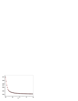
Figure 1: Average concurrence as a function of disorder strength parameter $\lambda$. Solid line is the fit curve of exponential decay. The system size $N=1600$ and the concurrence is averaged over 50 disorder ensembles.

To show the above result in more detail, we study the entanglement of ground state of the present one-dimensional disorder system by numerical calculations. In Fig. 1, the behavior of average concurrence of the ground state of Hamiltonian(5) versus disorder strength is presented. When the disorder is absent, i.e., $\lambda=0.0$, the average concurrence exhibits a maximal value. The increase of disorder strength leads to the decrease of average concurrence. It is shown that the decrease of concurrence fits the second exponential order

$$\left\langle C\right\rangle\sim B_{1}e^{-\lambda/D_{1}}+B_{2}e^{-\lambda/D_{2}}$$ (9)

with $B_{1}=0.00872,D_{1}=0.10611,B_{2}=0.00139,$ and $D_{2}=1.2166$. This numerical result indicates that the disorder has great effects on quantum entanglement, agreeing with the analytic result (8).In the extended case of Hamiltonian(5) , the system has a maximal entanglement so that this quantum correlation corresponds to an ideal electric conductor. When the disorder is introduced, the entanglement becomes small, the system turns from extended to localized state, and the conduction of system becomes finite and tends to be zero, indicating an insulator and no quantum correlation. If we consider the thermal conductivity carried by one spin excitation, the result is the same.

Figure 2: The distribution of the nearest-neighbor pairwise entanglement in the case of weak disorder.The system size $N=1600$.

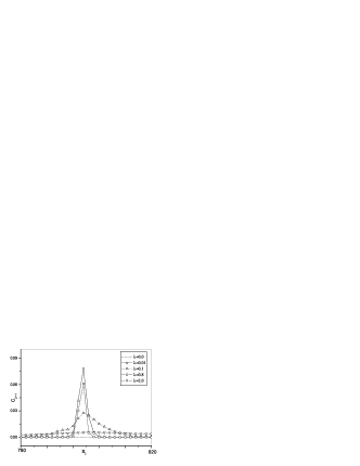
Figure 3: The distribution of the nearest-neighbor pairwise entanglement from weak disorder to strong disorder. The system size $N=1600$.

In fact, the disorder leads to spatial exponential decrease of eigenstates no matter how weak the disorder strength is MO . When a localization of state occurs, what will be the behaviors of pairwise entanglement? In the following, we will discuss the entanglement between two nearest-neighbor sites, and a distribution of the pairwise entanglement is expected. The concurrence for the nearest-neighbor sites $i$ and $i+1$ is given by $C_{i}=2\left|\psi_{i}\psi_{i+1}\right|$, and the numerical results are given in Fig. 2.

In Fig. 2, we notice that the entanglement distributes among every pair sites uniformly when the disorder is not present. Once the disorder is introduced, the localization emerges and the entanglement distribution becomes site-dependent. We can see that even the strength of disorder is very weak, for example $\lambda=0.01$, the entanglements between most of pairs are suppressed to a very small value and only some pair of sites exhibit higher pairwise entanglement around localization center. In other words, the entanglement is constrained to some certain pairs of sites. The distribution of pairwise entanglement with different values of $\lambda$ are plotted in Fig. 3. When $\lambda$ increases, the entanglements between more pairs of sites become close to zero, and the number of pairs which have enhanced pairwise entanglement becomes small. In other words, the width of localized entanglement distribution becomes small and entanglement is constrained. We can see that the localized entanglement is clear in the entanglement distribution picture.

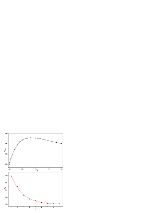
Figure 4: (a)The maximal pairwise entanglement as a function of disorder strength. $N=1600$ and $\gamma=0.1$.(b) The critical value of $\lambda$ as a function of relative index $j$ which label the distance from one site to the localization center site.

We also notice that the pairwise entanglement between localization center site and its near sites are firstly enhanced in the weak disorder regime and then suppressed in the strong disorder regime. This property is shown in Fig. 4(a), the entanglement $C_{i_{0}i_{0}+1}$ is plotted as the function of $\lambda$, where $i_{0}$ denote the localization center site. There exists a maximal value of entanglement at $\lambda=0.8.$ If $\lambda<0.8,$ the entanglement is increasing. When $\lambda$ is beyond $0.8$, the entanglement decreases linearly. Such behavior of the entanglement can be understood as following. On one side, the increase of $\lambda$ will lead to entanglement localization, thus enhance $C_{i_{0}i_{0}+1}$. On the other side, from Hamiltonian (5), we know that the increase of $\lambda$ will make the term $\sum_{i}V_{i}c_{i}^{\dagger}c_{i}$ predominant, which suppresses entanglement in the system. The competition between the two roles played by the disorder strength leads to the maximum value of the concurrence $C_{i_{0}i_{0}+1}$. We also study pairwise entanglements between non-nearest-neighbor sites and the center sites. They also present the maximal behavior during the increasing of disorder strength, but the critical value of $\lambda$ will decrease when the site is more far from the center site, which is shown is Fig. 4(b). $\lambda_{c}$ is plotted as the function of the index $j$, where $j$ is the relative index from the localization center and is defined as $j=i-i_{0}$, $i_{0}$ is the index of localization center. We note that the decrease of critical $\lambda$ is also exponential, which coincide with the the exponential decay of wavefunction.

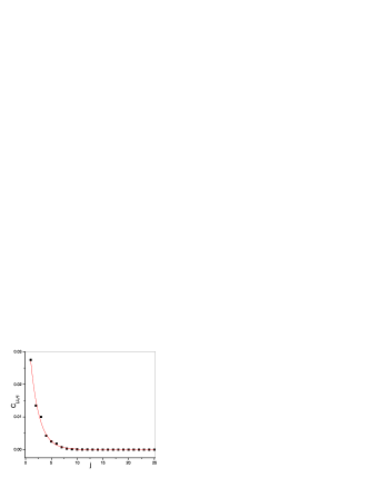
Figure 5: The pairwise entanglement between the center site of localization and $j$-th site, having distance $l=\left|x_{j}-x_{i_{0}}\right|$ from center site. Solid line is the fit curve of exponential decay. The size of the system $N=1600$.

We also consider the pairwise entanglement between the center site and it’s near sites when the disorder strength is fixed. In this case, the concurrence is given by $C_{j}=2\left|\psi_{j+i_{0}}\psi_{i_{0}}\right|$, where the label $j$ is the relative index from the localization center.As the amplitude of the wave function has the maximal absolute value at $x_{i_{0}}$, by considering Eq. (7), $C_{j}$ becomes $2|\psi_{i_{0}}^{2}|\exp(-|x_{j+i_{0}}-x_{i_{0}}|/\xi),$ which measures the entanglement between the localization center and $j$-th site away from the center. We calculate the entanglement and get the result with different disorder strengths. As expected, the pairwise entanglement decreases exponentially, agreeing with the simple analytical result. This property is shown in Fig. 5.

Figure 6: Time evolution of the average concurrence of present model with different disorder strength. The two extreme initial condition is applied (a)Zero entanglement initial state. (b) The maximal entanglement state.The system size $N=1600$.

From the above results of pairwise entanglement, we can find that when disorder is absent, the pairwise entanglement between every pair of sites is identical and independent on site index so that the nonlocality is completely shown. For spin system, one spin is entangled with the other one far from it as much as the one near it. This agrees with the result that in the extended state, the system is a perfect conductor for electric current or spin transport. If the strengthen of disorder is not zero, the pairwise entanglement becomes localizable and dependent on site index. The entanglement between nearest neighbor spins(sites) is different, and spins(sites) will prefer to entangle with near spins (sites) than the one far away. The nonlocality is destroyed, and entanglement is decrease globally, although some local entanglements between pair spins do not. In this case, one spin excitation would be pinned at some sites and the conduction vanishes.

We have studied the properties of ground-state entanglement in the one-dimensional Anderson disorder model. Next, we will investigate the dynamics of entanglement. This question can be solved by calculating the time-dependent Schrödinger equation

$$i\frac{d\psi_{i}}{dt}=-\psi_{i+1}-\psi_{i-1}+V_{i}\psi_{i}$$ (10)

which can be integrated numerically.

The dynamical behavior of average concurrence of presenting model are shown in Fig. 6 with different disorder strengths. Fig.6 (a) displays the dynamical evolution of entanglement with the initial state being $|\psi\rangle_{0}=|1\rangle=c_{l}^{\dagger}|0\rangle,$ where $l$, indicating one site of system. is set $l=N/2$ and $N$ is the size of system. In this case, the initial state has no entanglement, what will this state get entangled when time goes on? If disorder is absent, $\lambda=0,$ the average concurrence increases linearly with time. When time is long enough, the entanglement reaches a maximal value, after that it will decrease to a smaller value. When the disorder strength is not large, for example, $\lambda=0.05$, the entanglement also increase linearly at first stage and reach a maximal value. But the decrease of entanglement after maximal value becomes small. We notice that when $\lambda=0.1,$ the entanglement does not decrease, and almost keeps the maximal value. When disorder strength is large enough, like $\lambda=0.5$, the initial entanglement increases slowly. After reaching a small value, it does not increase again. If $\lambda$ is larger,for example $\left(\lambda=1.0\right),$ the entanglement exhibits almost no increase. This is a strong indicator of localization.

If one start the Equ. (10) from the maximally pairwise entangled initial state, namely the $W$ state MAa ; W , the dynamical behaviors are displayed in Fig 6. (b). The maximal entanglement is invariant while disorder is absent. But as soon as the disorder is introduced, the entanglement decreases as time goes on, the rate of the decrease is determined by the disorder strength. The larger disorder strength will make entanglement decrease quicker than smaller one. But it is interesting that no matter how large the disorder strength is, the entanglements will all decrease to a same residue value. Comparing the dynamical evolution of the entanglements from two different initial states, we find the asymptotic behaviors are different. The residue values of initial maximal entangled state are larger than those of initial non-entangled state for any value of disorder strength.

The evolution of entanglement in this system is determined by the diffusion of wavefunction and the localization. Without disorder, the wavefunction of electron will spread along the spatial direction. The external disorder potential can localize the motion of electron (or one excitation in XY spin system) on finite region of space. The existence of these two process leads to the dependence of evolution of entanglement on the initial condition and disorder strength. For an initial unentangled state which has a strong tendency to spread, a weak disorder can not prevent occupation possibility of particle sharing among more sites, so the entanglement will increase a lot, but a strong disorder will make a localization of the state, which leads to a small increase of entanglement. If the initial state is maximally entangled state, a completely extended state, so only the localization will determine the evolution entanglement. The entanglement must decrease as time goes on and the disorder strength determines the rate of decrease. We also do same calculations when we use other initial states different from the above two states. The result is also the same, namely, the disorder will destroy entanglement. By studying these properties, we can find that other states, except for ground state, have similar entanglement characters.So, it is true that electric conduction with single electron approximation and thermal conduction of one spin excitation are connected with quantum correlation measured by pairwise entanglement.

In summary, we have studied the ground state and dynamical pairwise entanglement of one-dimensional Anderson disorder model. By simple analytic and numerical results, we can find the entanglement is the indicator of localization caused by disorder. The disorder can destroy such quantum correlation. The relations between the entanglement and conduction are also discussed. On the other hand, we can localize one qubit on certain site by disorder, then we can do quantum operation on it.

It is interesting to consider entanglement in other disorder models. These studies will strength our understanding of entanglement, localization, and their relations. For instance, it is an interesting question to study effects of disorder on entanglement, the relation between localization and entanglement for other subspace with the number of electrons or spin excitations being large than one, which are under consideration. In that model , the effect of disorder on multi-party entanglement can also be investigated.

- (1) M.C. Arnesen, S. Bose, and V. Vedral, Phys. Rev. Lett. 87, 017901 (2001).
- (2) X. Wang, Phys. Rev. A 64, 012313 (2001).
- (3) K.M. O’Connor and W.K. Wootters, Phys. Rev. A 63, 052302 (2001).
- (4) D. Gunlycke, S. Bose, V.M. Kendon, and V. Vedral, Phys. Rev. A 64, 042302 (2001)
- (5) P. Zanardi, Phys. Rev. A, 65, 042101 (2002); P. Zanardi and X. Wang, J. Phys. A: Math. Gen. 35, 7947 (2002).
- (6) T.J. Osborne and M.A. Nielsen, Phys. Rev. A 66, 032110 (2002).
- (7) A. Osterloh, L. Amico, G. Falci, and R. Fazio, Nature(London) 416, 608 (2002).
- (8) F. Verstraete, M.A. Martin-Delgado,and J.I. Cirac, Phys. Rev. Lett. 92, 087201 (2004).
- (9) L.F. Santos, G. Rigolin and C.O. Escobar, Phy. Rev. A 69, 042304(2004); L. F. Santos, Phy. Rev. A 67, 062306(2003); O. Osenda, Z. Huang, and S. Kais, Phy. Rev. A 67, 062321(2003),L.F. Santos, M. I. Dykman, M. Shapiro and F. M. Lzrailev, Phy. Rev. A. 71,012317(2005)
- (10) Y. Shi, J.Phy.A 37,6807(2004),Y. Shi, Phys. Rev. A 67, 024301 (2003)
- (11) Y. Shi, Y. Shi, Phys. Lett. A 309, 254-261 (2003), Y. Shi, Phys. Rev. A 69, 032318 (2004)
- (12) A. Lakshminarayan and V. Subrahmanyam, Phy. Rev. A 67, 052304 (2003).
- (13) X. Wang, H. Li and B. Hu, Phy. Rev. A, 69,054303(2004).
- (14) H. Li, X. Wang and B. Hu,J. Phy. A: Math. Gen. 37,10665(2004) eprint quant-ph/0308116 (2003).
- (15) P.W. Anderson, Phys. Rev. 109, 1492 (1958).
- (16) S. Hill and W.K. Wootters, Phy. Rev. Lett. 78, 5022 (1997); W.K. Wootters, ibid. 80, 2245 (1998).
- (17) V. Coffman, J. Kundu, and W.K. Wootters, Phys. Rev. A 61, 052306 (2000).
- (18) P. Zanardi, Phys. Rev. A 65, 042101 (2002).
- (19) P.A. Lee and T.V. Ramakrishnan, Rev. Mod. Phys. 57, 287 (1985).
- (20) N.F. Mott and W. D. Twose, Adv. Phy. 10, 107 (1961); R.E. Borland, Proc. R. Soc. London Sev. A 274, 529 (1963).
- (21) W. Dür, G. Vidal, and J. I. Cirac, Phys. Rev. A62, 062314 (2000).