Quantum Memory Process with a Four-Level Atomic Ensemble

Abstract

We examine in detail the quantum memory technique for photons in a double $\Lambda$ atomic ensemble in this work. The novel application of the present technique to create two different quantum probe fields as well as entangled states of them is proposed. A larger zero-degeneracy class besides dark-state subspace is investigated and the adiabatic condition is confirmed in the present model. We extend the single-mode quantum memory technique to the case with multi-mode probe fields, and reveal the exact pulse matching phenomenon between two quantized pulses in the present system.

I introduction

Since the remarkable demonstration of ultraslow light speed in a Bose-Einstein condensate in 1999 1 , rapid advances have been witnessed in both experimental and theoretical aspects towards probing the novel mechanism of Electromagnetically Induced Transparency (EIT) 2 and its many potential applications 3 ; 4 ; 5 ; entangled ; wu . Particularly, based on “dark-state polaritons” (DSPs) theory 6 , the quantum memory via EIT technique is actively being explored by transferring the quantum states of photon wave-packets to metastable collective atomic-coherence (collective quasi spin states) in a loss-free and reversible manner 7 . For the three-level EIT quantum memory technique, a semidirect product group under the condition of large atom number and low collective excitation limit 6 was discovered by Sun $etal.$ 8 , and the validity of the adiabatic condition for the evolution of DSPs has also been confirmed.

As a natural extension, controlled light storing in a medium composed of double $\Lambda$ type four-level atoms was mentioned 9 and briefly studied recently 10 . However, in these previous theoretical works, the probe light is treated as classical10 and the evolution of the total wave function of the probe pulses and atoms is not clear. Thus many properties of quantum memory with four-level atomic system have not been discovered. In this paper, we present a quantum description of DSP theory in such a double $\Lambda$ type atomic ensemble interacting with two quantized fields and two classical control fields. The novel application of our model to create two different quantum probe fields as well as their entangled states is proposed. Furthermore, we extend the single-mode quantum memory technique to the case with multi-mode probe fields, and reveal the exact pulse matching phenomenon between two quantized probe pulses.

II model

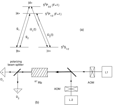
Figure 1: Double $\Lambda$ type four-level ⁸⁷Rb atoms coupled to two single-mode quantized and two classical control fields (a). The schematic setup for experimental realization is shown in part (b). Co-propagating input probe and control fields are used to avoid Doppler-broadening. The polarizing beam splitter is used to separate probe photons from control ones.

Turning to the situation of Fig. 1(a), we assume that a collection of $N$ double $\Lambda$ type four-level atoms (⁸⁷Rb) interact with two single-mode quantized fields with coupling constants $g_{1}$ and $g_{2}$, and two classical control ones with time-dependent real Rabi-frequencies $\Omega_{1}(t)$ and $\Omega_{2}(t)$. Generalization to the multi-mode probe pulse case will be studied later. All probe and control fields are co-propagating in the $z$ direction (Fig. 1(b)). Considering all transitions at resonance, the interaction Hamiltonian of the total system can be written as:

$$\hat{V}=g_{1}\sqrt{N}\hat{a}_{1}\hat{A}^{{\dagger}}+\Omega_{1}\hat{T}_{ac}+g_{2}\sqrt{N}\hat{a}_{2}\hat{D}^{{\dagger}}+\Omega_{2}\hat{T}_{dc}+h.c.,$$ (1)

where the collective atomic excitation operators: $\hat{A}=\frac{1}{\sqrt{N}}\sum_{j=1}^{N}\hat{\sigma}_{ba}^{j},\ \hat{C}=\frac{1}{\sqrt{N}}\sum_{j=1}^{N}\hat{\sigma}_{bc}^{j},\ \hat{D}=\frac{1}{\sqrt{N}}\sum_{j=1}^{N}\hat{\sigma}_{bd}^{j}$ with $\hat{\sigma}^{i}_{\mu\nu}=|\mu\rangle_{ii}\langle\nu|(\mu,\nu=a,b,c,d)$ being the flip operators of the $i$-th atom between states $|\mu\rangle$ and $|\nu\rangle$, and $\hat{T}^{-}_{\mu\nu}=\hat{T}_{\mu\nu}=\sum_{j=1}^{N}\hat{\sigma}_{\mu\nu}^{j},\ \ \hat{T}_{\mu\nu}^{+}=(\hat{T}^{-}_{\mu\nu})^{\dagger}$ with $\mu\neq\nu=a,c,d$. Denoting by $|b\rangle=|b_{1},b_{2},...,b_{N}\rangle$ the collective ground state with all $N$ atoms staying in the same single particle ground state $|b\rangle$, we can easily give other quasi-spin wave states by the collective atomic excitation operators: $|a^{n}\rangle=[n!]^{-1/2}(\hat{A}^{{\dagger}})^{n}|b\rangle$, $|c^{n}\rangle=[n!]^{-1/2}(\hat{C}^{{\dagger}})^{n}|b\rangle$, and $|d^{n}\rangle=[n!]^{-1/2}(\hat{D}^{{\dagger}})^{n}|b\rangle$. Following the analysis in ref. 8 , one can verify that the dynamical symmetry of our double $\Lambda$ system is governed by a semidirect sum Lie algebra $su(3)\overline{\otimes}h_{3}$ in large $N$ limit and low excitation condition.

To give a clear description of the interesting quantum memory process in this double $\Lambda$ type four-level-atoms ensemble, we define the new type of dark-state-polaritons operator as

$$\hat{d}=\cos\theta\cos\phi\hat{a}_{1}-\sin\theta\hat{C}+\cos\theta\sin\phi\hat{a}_{2},$$ (2)

where the mixing angles $\theta$ and $\phi$ are defined through $\tan\theta=g_{1}\sqrt{N}/\sqrt{\Omega_{1}^{2}+\Omega_{2}^{2}g_{1}^{2}/g_{2}^{2}}$ and $\tan\phi=g_{1}\Omega_{2}/g_{2}\Omega_{1}$. By a straightforward calculation one can verify that $[\hat{d},\hat{d}^{{\dagger}}]=1$ and $[\hat{V},\hat{d}\ ]=0$, hence the general atomic dark states can be obtained through $|D_{n}\rangle=[n!]^{-1/2}(\hat{d}^{{\dagger}})^{n}|0\rangle$, where $|0\rangle=|b\rangle\otimes|0,0\rangle_{e}$ and $|0,0\rangle_{e}$ denotes the electromagnetic vacuum of two quantized probe fields. So we reach

$$|D_{n}\rangle = \sum^{n}_{k=0}\sum^{n-k}_{j=0}\sqrt{\frac{n!}{k!(n-k-j)!j!}}(-\sin\theta)^{k}(\cos\theta)^{n-k}$$ (3)

$$(\sin\phi)^{j}(\cos\phi)^{n-k-j}|c^{k},n-k-j,j\rangle.$$

From this formula it is clear that when the mixing angle $\theta$ is adiabatically rotated from $0$ to $\pi/2$, the quantum state of the DSPs is transferred from pure photonic character to collective excitations, i.e. $|D_{n}\rangle:\ \sum^{n}_{j=0}\sqrt{\frac{n!}{(n-j)!j!}}(\sin\phi)^{j}(\cos\phi)^{n-j}|b\rangle|n-j,j\rangle\rightarrow|c^{n}\rangle|0,0\rangle$.

Similarly, another important physical phenomenon can also be predicted through our quantized description of this system. If initially only one quantized field (described by the coherent state $|\alpha_{2}\rangle$ with $\alpha_{2}=\alpha_{0}$) is injected into the atomic ensemble to couple the transition from $|b\rangle$ to $|d\rangle$, and the second control field is chosen to be much stronger than the first one $(g_{1}\Omega_{2}(0)\gg g_{2}\Omega_{1}(0))$ along with $\sqrt{g_{2}^{2}\Omega_{1}^{2}(0)+g_{1}^{2}\Omega_{2}(0)^{2}}\gg g_{1}g_{2}\sqrt{N}$ (or $\sin\phi_{0}=1$ and $\cos\theta_{0}=1$), the initial total state of the quantized field and atomic ensemble reads

$$|\Psi_{0}\rangle=\sum_{n}P_{n}(\alpha_{0})|0,n\rangle\otimes|b\rangle,$$ (4)

where $P_{n}(\alpha_{0})=\frac{\alpha_{0}^{n}}{\sqrt{n!}}e^{-|\alpha_{0}|^{2}/2}$ is the probability distribution function. Subsequently, the mixing angle $\theta$ is adiabatically rotated to $\pi/2$ by turning off the two control fields, hence the quantum state of the probe light $|\alpha_{2}\rangle$ is fully mapped into the collective atomic excitations. When both of the two control fields are turned back on and the mixing angle $\theta$ is rotated to $\theta=0$ again with $\phi$ to some value $\phi_{e}$, which is only determined by the Rabi-frequencies of the two re-applied control fields, we finally obtain from eq.(3)

$$|\Psi_{e}\rangle = \sum_{j}\sum_{k}P_{j}(\alpha_{e1})P_{k}(\alpha_{e2})|b,j,k\rangle$$ (5)

$$=|b\rangle\otimes|\alpha_{e1}\rangle\otimes|\alpha_{e2}\rangle,$$

where $\alpha_{e1}=\alpha_{0}\cos\phi_{e}$ and $\alpha_{e2}=\alpha_{0}\sin\phi_{e}$ are the parameters of the two released coherent lights. The above expression shows that the injected quantized field can convert into two different coherent pulses $|\alpha_{ei}\rangle(i=1,2)$ after a proper evolution manipulated by two control fields. For example, i) if $\phi_{e}=\pi/2$, we have $\alpha_{e1}=0$ and $\alpha_{e2}=\alpha_{0}$, which means the released pulse is the same as the initial injected one; ii) if $\phi_{e}=0$, we have $\alpha_{e1}=\alpha_{0}$ and $\alpha_{e2}=0$, which means that the injected quantized field state is now fully converted into a different light beam $|\alpha_{e1}\rangle$. Obviously, this novel mechanism can be extended to other cases of the injected field, for example, in the presence of a non-classical or squeezed light beam (see the following discussion). In experiments, there also holds the promise for actual observation through, e.g., combining a beam splitter and an electro-optic modulator to generate the requisite sidebands 1 .

III generation of entangled coherent states

It is interesting to note that when we input a non-classical or squeezed probe light, by proper steering the control fields, we can generate two output entangled light beams. Firstly we consider that the injected quantized field is in a macroscopic quantum superposition of coherent states, e.g. for the initial total state

$$|\Psi_{0}\rangle^{\pm}=\frac{1}{\sqrt{{\cal N}(\alpha_{0})}}|0\rangle\otimes(|\alpha_{0}\rangle\pm|-\alpha_{0}\rangle)\otimes|b\rangle,$$ (6)

where the normalized factor ${\cal N}_{\pm}(\alpha_{0})=2\pm 2e^{-2|\alpha_{0}|^{2}}$, with the scheme discussed above and from eq. (3) we find the injected quantized pulse can evolve into a very interesting entangled coherent state (ECS) of two output fields ($|\Psi_{0}\rangle^{\pm}\rightarrow|\Psi_{e}\rangle^{\pm}$)

$$\frac{1}{\sqrt{{\cal N}_{\pm}(\alpha_{0})}}|0\rangle\otimes\bigr{(}|\alpha_{0}\rangle\pm|-\alpha_{0}\rangle\bigr{)}\otimes|b\rangle=\frac{1}{\sqrt{{\cal N}_{\pm}(\alpha_{0})}}\bigr{(}|0\rangle\otimes|\alpha_{0}\rangle\pm|0\rangle\otimes|-\alpha_{0}\rangle\bigr{)}\otimes|b\rangle\longrightarrow$$

$$\longrightarrow\frac{1}{\sqrt{{\cal N}_{\pm}(\alpha_{0})}}\bigr{(}\sum_{j}\sum_{k}P_{j}(\alpha_{e1})P_{k}(\alpha_{e2})|b,j,k\rangle\pm\sum_{j}\sum_{k}P_{j}(-\alpha_{e1})P_{k}(-\alpha_{e2})|b,j,k\rangle\bigr{)}.$$ (7)

The final state in the above formula can be rewritten as:

$$|\Psi_{e}\rangle^{\pm}=\frac{1}{\sqrt{{\cal N}_{\pm}(\alpha_{0})}}\bigr{(}|\alpha_{e1},\alpha_{e2}\rangle\pm|-\alpha_{e1},-\alpha_{e2}\rangle\bigr{)}_{light}\otimes|b\rangle.$$ (8)

where the subscript $light$ indicates the state of the output two probe pulses.

If $\phi_{e}=0$, hence $\alpha_{e1}=\alpha_{0}$ and $\alpha_{e2}=0$, and then the evolution of the quantized fields proceeds as $|0\rangle\otimes(|\alpha_{0}\rangle\pm|-\alpha_{0}\rangle)/\sqrt{{\cal N}_{\pm}(\alpha_{0})}\rightarrow(|\alpha_{0}\rangle\pm|-\alpha_{0}\rangle)\otimes|0\rangle/\sqrt{{\cal N}_{\pm}(\alpha_{0})}$, which means the input Schrödinger state is now fully converted into another one with different vibrational mode. On the other hand, for the general case of non-zero value of the coherent parameters $\alpha_{e1}$ and $\alpha_{e2}$, the states of output quantized fields are entangled coherent states. Since the parameters $\alpha_{ei}(i=1,2)$ are controllable, the entanglement of the output states entanglement $E^{\pm}(\alpha_{e1},\alpha_{e2})=-$ tr$(\rho^{\pm}_{\alpha_{e1}}\ln\rho^{\pm}_{\alpha_{e1}})$ with the reduced density matrix $\rho^{\pm}_{\alpha_{e1}}=$ tr${}^{(\alpha_{e2},atom)}(|\Psi_{e}\rangle\langle\Psi_{e}|)^{\pm}$ can also easily be controlled by the re-applied control fields. In particular, for the initial state $|\Psi_{0}\rangle^{-}$, if $\phi_{e}=\pi/4$, we have $\alpha_{e1}=\alpha_{e2}=\alpha_{0}/\sqrt{2}$ and then we obtain the maximally entangled state(MES):

$$|0\rangle\otimes\bigr{(}|\alpha_{0}\rangle-|-\alpha_{0}\rangle\bigr{)}/\sqrt{{\cal N}_{-}(\alpha_{0})}\longrightarrow$$ (9)

$$\longrightarrow\bigr{(}|\frac{\alpha_{0}}{\sqrt{2}},\frac{\alpha_{0}}{\sqrt{2}}\rangle-|-\frac{\alpha_{0}}{\sqrt{2}},-\frac{\alpha_{0}}{\sqrt{2}}\rangle\bigr{)}/\sqrt{{\cal N}_{-}(\alpha_{0})},$$

which is most useful for quantum information processes. With the definitions of the orthogonal basis $|+\rangle=\bigr{(}|\frac{\alpha_{0}}{\sqrt{2}}\rangle+|-\frac{\alpha_{0}}{\sqrt{2}}\rangle\bigr{)}/\sqrt{{\cal N}_{+}(\alpha_{0}/2)}$ and $|-\rangle=\bigr{(}|\frac{\alpha_{0}}{\sqrt{2}}\rangle-|-\frac{\alpha_{0}}{\sqrt{2}}\rangle\bigr{)}/\sqrt{{\cal N}_{-}(\alpha_{0}/2)}$, the output coherent states can be rewritten as

$$\Phi_{light}(-)=\frac{1}{\sqrt{2}}\bigr{(}|+\rangle|-\rangle+|-\rangle|+\rangle\bigr{)}_{light},$$ (10)

which manifestly has one ebit of entanglement (since $\langle+|-\rangle=0$). We should emphasize that all the above results can not be obtained with classical DSP theory of a four-level system. Since our scheme of generating the entangled coherent states via quantized DSP theory is linear and controllable and it only requires a macroscopic quantum superposition for the initial state, this scheme may be feasible in experiment which has made much progress in recent years ent . Besides our technique, the generation of entangled coherent states via Kerr effect entangled and entanglement swapping using Bell-state measurements swap is also studied widely.

If the two output entangled coherent lights are respectively injected into two other atomic ensembles composed of many three-level atoms, and the quantum states of the lights are mapped into quasi spin-waves via sperate Raman transitions, it is possible to generate controllable entangled coherence of two atomic ensembles.

Consider now a different type of input quantum state corresponding to a single-photon state, i.e. the initial total state $|\Psi_{0}\rangle=(|0\rangle\otimes|1\rangle)_{light}\otimes|b\rangle$. According to Eq. (3) and after the light state storage process discussed in section II, the final state yields:

$$\Phi_{light}=\frac{1}{\sqrt{2}}\bigr{(}|1\rangle|0\rangle+|0\rangle|1\rangle\bigr{)}_{light}.$$ (11)

The entangled states generated with the present scheme have other interesting aspects. Firstly, since the two output probe fields are different in frequency, the generated entangled states is between two quantized fields with different frequencies. Secondly, since the direction of the output probe field can be fully controlled by the corresponding control field 3 , based on our scheme, the output directions of the two entangled probe fields can be controlled by the two reapplied control fields. These interesting factors are advantages of our scheme for generating entangled light fields, which is different from that using a standard beam splitter.

IV validity of adiabatic condition

As we have known, the condition of adiabatic evolution is most important for the quantum memory technique based on the quantized DSPs theory, because the total system should be confined to the dark states during the process of quantum memory. One can verify that when $g_{1}\neq g_{2}$, no larger zero subspace is obtained except for dark states and the adiabatic condition can be guaranteed by the adiabatic theorem. However, the dynamical symmetry in the present system depicted by the semi-direct sum algebra $h_{3}\overline{\otimes}su(3)$ indicates that, for the special case $g_{1}=g_{2}=g$, we may find a larger degeneracy class of states with zero-eigenvalue in this system. We define

$$\hat{Q}_{\pm}^{{\dagger}}=\hat{u}^{{\dagger}}\pm\hat{b}^{{\dagger}},\ \ \hat{P}_{\pm}^{{\dagger}}=-\sin\phi\hat{a}_{1}+\cos\phi\hat{a}_{2}\pm\hat{v}^{{\dagger}},$$ (12)

where the operators $\hat{u}$, $\hat{v}$ and the bright-state-polaritons (BSPs) operator $\hat{b}$ are defined as: $\hat{u}=\cos\phi\hat{A}+\sin\phi\hat{D},\ \hat{v}=-\sin\phi\hat{A}+\cos\phi\hat{D}$ and $\hat{b}=\sin\theta\cos\phi\hat{a}_{1}+\cos\phi\hat{C}+\sin\theta\sin\phi\hat{a}_{2}$. By a straightforward calculation one obtains the communication relations $[\hat{V},\hat{Q}_{\pm}^{{\dagger}}]=\pm\epsilon_{1}\hat{Q}_{\pm}^{{\dagger}}$, $[\hat{V},\hat{P}^{{\dagger}}]=\pm\epsilon_{2}\hat{P}_{\pm}^{{\dagger}}$ and $[\hat{P}_{\pm}^{{\dagger}},\hat{Q}_{\pm}^{{\dagger}}]=0$ with $\epsilon_{1}=\sqrt{g^{2}N+\Omega_{1}^{2}+\Omega_{2}^{2}}$ and $\epsilon_{2}=g\sqrt{N}$. Thus we further obtain

$$[\hat{V},\hat{P}_{\pm}^{{\dagger}}\hat{Q}_{\pm}^{{\dagger}}]=\pm\epsilon_{1}\hat{P}_{\pm}^{{\dagger}}\hat{Q}_{\pm}^{{\dagger}}\pm\epsilon_{2}\hat{P}_{\pm}^{{\dagger}}\hat{Q}_{\pm}^{{\dagger}}$$ (13)

To this end we have obtained all communication relations between the above operators. Thanks to these results we finally obtain a much larger degeneracy class:

$$|r(i,j;k,l;n)\rangle=\frac{1}{\sqrt{i!j!k!l!}}(\hat{Q}_{+}^{{\dagger}})^{i}(\hat{Q}_{-}^{{\dagger}})^{j}(\hat{P}_{+}^{{\dagger}})^{k}(\hat{P}_{-}^{{\dagger}})^{l}|D_{n}\rangle,$$

with eigenvalue $E(i,j;k,l)=(i-j)\epsilon_{1}+(k-l)\epsilon_{2}$. Obviously, when $i=j$ and $k=l$, one finds the zero-eigenvalue degeneracy class is

$$|d(i,k;n)\rangle = \frac{1}{i!k!}(\hat{Q}_{+}^{{\dagger}}\hat{Q}_{-}^{{\dagger}})^{i}(\hat{P}_{+}^{{\dagger}}\hat{P}_{-}^{{\dagger}})^{k}|D_{n}\rangle,$$

$$(i,k,n=0,1,2,\cdots).$$

The larger class $\{|d(i,k;n)\rangle\ |$ $\ n=0,1,2,\cdots\}$ of states of zero eigenvalue are constructed by acting ($\hat{Q}_{+}^{{\dagger}}\hat{Q}_{-}^{{\dagger}}$) $i$ times and ($\hat{P}_{+}^{{\dagger}}\hat{P}_{-}^{{\dagger}}$) $k$ times on the dark state $|D_{n}\rangle$. Only when $i=0$ and $k=0$, the larger degeneracy class reduces to the special subset $\{|D_{n}\rangle\ |$$n=0,1,2,\cdots\}$ of the interaction Hamiltonian. As usual, the quantum adiabatic theorem does not forbid the transition between those states of same eigenvalue, hence it is important also in the present four-level-atoms system to confirm the forbiddance of any transitions from dark states $|D_{n}\rangle$ to $\{|d(i,k;n)\rangle\ |ik\neq 0,n=0,1,2,\cdots\}$. Generally this problem can be studied by defining the zero-eigenvalue subspaces ${\bf S}^{[i,k]}:\{|d(i,k;n)\rangle\ |i,k,n=0,1,2,\cdots\}$, in which ${\bf S}^{[0,0]}={\bf S}$ is the dark-state subspace. The complementary part of the direct sum ${\bf DS}={\bf S}^{[0,0]}\oplus$ ${\bf S}^{[0,1]}\oplus$ ${\bf S}^{[1,0]}\oplus\cdots$ of all zero-eigenvalue subspaces is noted by ${\bf ES}={\bf S}^{[\bf ES]}$ in which each state turns out to have some nonzero eigenvalue after some calculations. Any state $|\phi^{[i,k]}(t)\rangle=\sum_{i,k;n}c_{n}^{[i,k]}(t)|d(i,k;n)\rangle$ in ${\bf S}^{[i,k]}$ evolves according to 8

$$i\frac{d}{dt}c_{n}^{[i,k]}(t)=\sum_{i^{\prime},k^{\prime};n^{\prime}}D_{i,k;n}^{i^{\prime},k^{\prime};n^{\prime}}c_{n^{\prime}}^{[i^{\prime},k^{\prime}]}(t)+F[{\bf ES}],$$ (15)

where $F[{\bf ES}]$, which can be ignored under adiabatic conditions 8 ; 11 , represents a certain functional of the complementary states and $D_{i,k;n}^{i^{\prime},k^{\prime};n^{\prime}}=-i\langle d(i^{\prime},k^{\prime};n^{\prime})|\partial_{t}|d(i,k;n)\rangle=-i\dot{\theta}\langle d(i^{\prime},k^{\prime};n^{\prime})|\partial_{\theta}|d(i,k;n)\rangle-i\dot{\phi}\langle d(i^{\prime},k^{\prime};n^{\prime})|\partial_{\phi}|d(i,k;n)\rangle$ with $\dot{\theta}=d\theta/dt$ and $\dot{\phi}=d\phi/dt$. With the definitions of these operators, we can easily calculate:

$$\partial_{\theta}\hat{b}=\hat{d},\ \partial_{\theta}\hat{d}=-\hat{b};$$

$$\partial_{\phi}\hat{b}=\sin\theta\hat{s},\ \partial_{\phi}\hat{u}=\hat{v},$$ (16)

$$\partial_{\phi}\hat{v}=-\hat{u},\ \partial_{\phi}\hat{a}=\hat{s},\ \partial_{\phi}\hat{s}=-\hat{a},$$

where $\hat{a}=\cos\phi\hat{a}_{1}+\sin\phi\hat{a}_{2}$ and $\hat{s}=-\sin\phi\hat{a}_{1}+\cos\phi\hat{a}_{2}$. From these results one can finally determine that the equations about $\partial_{\theta}|d(i,k;n)\rangle$ and $\partial_{\phi}|d(i,k;n)\rangle$ do not contain the term $|d(i^{\prime},k^{\prime};n^{\prime})\rangle$, hence $\langle d(i^{\prime},k^{\prime};n^{\prime})|\partial_{t}|d(i,k;n)\rangle=0$ and the evolution equation yields $\frac{d}{dt}c_{n}^{[i,k]}(t)=0$, i.e., there is no mixing of different zero-eigenvalue subspaces during the adiabatic process and therefore, even for the special case of $g_{1}=g_{2}$, quantum memory may till be robust in the present double $\Lambda$ type atomic ensemble.

V quantum memory for multi-mode quantized fields

In this section we shall extend the technique of quantum memory for a single-mode field to the multi-mode case in the double $\Lambda$ atomic-ensemble system. The two quantized fields described by the slowly-varying dimensionless operator are given by

$$\hat{\cal E}_{j}(z,t)=\sum_{k}\hat{a}_{k_{j}}(t){\rm e}^{-i\frac{\nu_{j}}{c}(z-ct)},\ (j=1,2),$$ (17)

where $\nu_{1}=\omega_{ab},\nu_{2}=\omega_{db}$ are the carrier frequencies of the two quantized optical fields. If the (slowly-varying) quantum amplitude does not change much in a small length interval $\Delta z$ which contains $N_{z}\gg 1$ atoms, we can introduce continuous atomic variables 6

$$\widetilde{\sigma}_{\mu\nu}(z,t)=\frac{1}{N_{z}}\sum_{z_{j}\in N_{z}}{\hat{\sigma}}_{\mu\nu}^{j}(t),$$ (18)

where $\hat{\sigma}_{\mu\nu}^{j}=|\mu_{j}\rangle\langle\nu_{j}|\,{\rm e}^{-i\frac{\omega_{\mu\nu}}{c}(z-ct)}$ is the slowly-varying part of the atomic flip operators. Making the replacement $\sum_{j=1}^{N}\longrightarrow\frac{N}{L}\int{\rm d}z$ with $L$ the length of the interaction in the propagation direction of the quantized field, the interaction Hamiltonian then yields

$${\hat{V}} = -\int\frac{dz}{L}\bigr{(}\hbar g_{1}N\widetilde{\sigma}_{ab}(z,t)\hat{\cal E}_{1}(z,t)+\hbar\Omega_{1}(t)N\widetilde{\sigma}_{ac}(z,t)$$

$$+\hbar g_{2}N\widetilde{\sigma}_{db}(z,t)\hat{\cal E}_{2}(z,t)+\hbar\Omega_{2}(t)N\widetilde{\sigma}_{dc}(z,t)$$

$$+h.a\bigr{)}.$$

The evolution of the Heisenberg operators $\hat{\cal E}_{i}(z,t)$ corresponding to the two quantum fields can be described by the propagation equations

$$\left(\frac{\partial}{\partial t}+c\frac{\partial}{\partial z}\right)\hat{\cal E}_{1}(z,t)=ig_{1}N\widetilde{\sigma}_{ba}(z,t)$$ (20)

and

$$\left(\frac{\partial}{\partial t}+c\frac{\partial}{\partial z}\right)\hat{\cal E}_{2}(z,t)=ig_{2}N\widetilde{\sigma}_{bd}(z,t).$$ (21)

In the condition of low excitation, i.e. $\widetilde{\sigma}_{bb}\approx 1$, the atomic evolution governed by the Heisenberg-Langevin equations can be obtained by

$$\dot{\widetilde{\sigma}}_{ba}=-\gamma_{ba}{\widetilde{\sigma}}_{ba}+ig_{1}\hat{\cal E}_{1}+i\Omega_{1}{\widetilde{\sigma}}_{bc}+F_{ba},$$ (22)

$$\dot{\widetilde{\sigma}}_{bc}=i\Omega_{1}{\widetilde{\sigma}}_{ba}-ig_{1}\hat{\cal E}_{1}{\widetilde{\sigma}}_{ac}+i\Omega_{2}{\widetilde{\sigma}}_{bd}-ig_{2}\hat{\cal E}_{2}{\widetilde{\sigma}}_{dc},$$ (23)

$$\dot{\widetilde{\sigma}}_{bd}=-\gamma_{bd}{\widetilde{\sigma}}_{bd}+ig_{2}\hat{\cal E}_{2}+i\Omega_{2}{\widetilde{\sigma}}_{bc}+F_{bd},$$ (24)

where $\gamma_{\mu\nu}$ are the transversal decay rates that will be assumed $\gamma_{ba}=\gamma_{bd}=\Gamma$ in the following derivation and $F_{\mu\nu}$ are $\delta$-correlated Langevin noise operators. From Eqs. (22) and 24 we find in the lowest (zero) order

$${\widetilde{\sigma}}_{ba}=(ig_{1}\hat{\cal E}_{1}+i\Omega_{1}{\widetilde{\sigma}}_{bc}+F_{ba})/\Gamma,$$ (25)

$${\widetilde{\sigma}}_{bd}=(ig_{2}\hat{\cal E}_{2}+i\Omega_{2}{\widetilde{\sigma}}_{bc}+F_{bd})/\Gamma.$$ (26)

Substitute the above two formulae into Eq. (23) yields

$$\dot{\widetilde{\sigma}}_{bc}=\Gamma^{-1}\Omega_{0}^{2}{\widetilde{\sigma}}_{bc}-\Gamma^{-1}(g_{1}\Omega_{1}\hat{\cal E}_{1}+g_{2}\Omega_{2}\hat{\cal E}_{2}),$$ (27)

where $\Omega_{0}=\sqrt{\Omega_{1}^{2}+\Omega_{2}^{2}}$. The Langevin noise terms are neglected in the above results. For our purpose we shall calculate $\widetilde{\sigma}_{bc}$ to the first order, so

$$\widetilde{\sigma}_{bc}\approx-\frac{1}{\Omega_{0}^{2}}(g_{1}\Omega_{1}\hat{\cal E}_{1}+g_{2}\Omega_{2}\hat{\cal E}_{2})+$$

$$+\frac{\Gamma}{\Omega_{0}^{4}}(g_{1}\Omega_{1}\partial_{t}\hat{\cal E}_{1}+g_{2}\Omega_{2}\partial_{t}\hat{\cal E}_{2}).$$ (28)

According to the former discussions, here the dark- and bright-state polaritons in the multi-mode case can be defined in continuous form:

$$\hat{\Psi}(z,t)=\cos\theta(t)\hat{\cal E}_{12}(z,t)-\sin\theta(t)\,\sqrt{N}\,\widetilde{\sigma}_{bc}(z,t),$$ (29)

$$\hat{\Phi}(z,t)=\sin\theta(t)\hat{\cal E}_{12}(z,t)+\cos\theta(t)\,\sqrt{N}\,\widetilde{\sigma}_{bc}(z,t),$$ (30)

where $\hat{\cal E}_{12}(z,t)=\cos\phi(t)\,\hat{\cal E}_{1}(z,t)+\sin\phi(t)\,\hat{\cal E}_{2}(z,t)$ is the superposition of two quantized probe fields.

One can transform the equations of motion for the electric field and the atomic variables into the new field variables. Similar to the single-mode case, we consider the low-excitation approximation and find

$$\biggl{[}\frac{\partial}{\partial t}+c\cos^{2}\theta\frac{\partial}{\partial z}\biggr{]}\,\hat{\Psi}(z,t)=\dot{\phi}\sin\theta\cos^{2}\theta\,\hat{s}(z,t)-$$

$$-\dot{\theta}\,\hat{\Phi}(z,t)-\sin\theta\cos\theta\,c\frac{\partial}{\partial z}\hat{\Phi}(z,t),$$ (31)

and

$$\Phi = \frac{\Gamma}{g_{1}g_{2}\sqrt{N}}\frac{\cos^{2}\theta}{\Omega^{2}_{0}}\tan\theta\frac{\partial}{\partial t}(\sin\theta\Psi-\cos\theta\Phi)$$ (32)

$$-\sin\theta(\Omega_{2}^{2}-\Omega_{1}^{2})\hat{s}(z,t),$$

where we have defined $\hat{s}(z,t)=-\sin\phi(t)\,\hat{\cal E}_{1}(z,t)+\cos\phi(t)\,\hat{\cal E}_{2}(z,t)$. It is easy to see when $\hat{s}=0$, the total system can be reduced to the usual three-level one. For this we shall calculate the equation of motion of $\hat{s}(z,t)$ to study the adiabatic condition. From Eqs. (20) and (21) and together with the results of ${\widetilde{\sigma}}_{ba}$ and ${\widetilde{\sigma}}_{bd}$ one can verify that

$$(\frac{\partial}{\partial t}+c\cos^{2}\beta\frac{\partial}{\partial z})\hat{s} = -\frac{(g_{1}^{2}\Omega_{2}^{2}+g_{2}^{2}\Omega_{1}^{2})N}{\Gamma}\frac{\cos^{2}\beta}{\Omega_{0}^{2}}\hat{s}-$$ (33)

$$-\frac{1}{2}g_{1}g_{2}\sqrt{N}\sin 2\beta\frac{\partial}{\partial t}\hat{\cal E}_{12},$$

with

$$\tan^{2}\beta=\frac{N\Omega_{1}^{2}\Omega_{2}^{2}}{g_{1}^{2}\Omega_{2}^{2}+g_{2}^{2}\Omega_{1}^{2}}\frac{(g_{1}^{2}-g_{2}^{2})^{2}}{\Omega_{0}^{2}}.$$ (34)

The time derivative of the mixing angle $\phi$ is neglected in the above equation. The first term in the right side of Eq. (33) reveals a large absorption of $\hat{s}(z,t)$, which causes the field $\hat{s}(z,t)$ to be quickly reduced to zero so that the present system reaches pulse matching 10 ; match ; liu : $\hat{\cal E}_{2}\rightarrow\tan\phi\hat{\cal E}_{1}$. For a numerical estimation, we typically set 3 $g_{1}\approx g_{2}\sim 10^{5}s^{-1},N\approx 10^{8}$, $\Gamma\approx 10^{8}s^{-1}$, then the life time of field $\hat{s}(z,t)$ is about $\Delta t\sim 10^{-10}s$ which is much smaller than the storage time 3 . Furthermore, by introducing the adiabaticity parameter $\tau=(g_{1}g_{2}\sqrt{N}T/\Gamma)^{-1}$, we calculate the lowest order in Eq. (32) and thus obtain $\hat{\Phi}\approx 0,\hat{s}\approx 0$. Then the formula (V) reduces to the motion equation of DSPs defined in the usual three-level $\Lambda$ type system. Consequently we have

$$\hat{\cal E}_{1}(z,t)=\cos\theta(t)\cos\phi(t)\hat{\Psi}(z,t)$$ (35)

$$\hat{\cal E}_{2}(z,t)=\cos\theta(t)\sin\phi(t)\hat{\Psi}(z,t)$$ (36)

$$\sqrt{N}\widetilde{\sigma}_{bc}(z,t)=-\sin\theta(t)\hat{\Psi}(z,t)$$ (37)

where $\hat{\Psi}$ obeys the very simple equation of motion

$$\biggl{[}\frac{\partial}{\partial t}+c\cos^{2}\theta\frac{\partial}{\partial z}\biggr{]}\,\hat{\Psi}(z,t)=0$$ (38)

The above results clearly show that, for example, if the initial condition reads $\theta\rightarrow 0$ and $\phi\rightarrow 0$, i.e. initially the external control fields are much stronger $\sqrt{g_{2}^{2}\Omega_{1}^{2}+g_{1}^{2}\Omega_{2}^{2}}\gg g_{1}g_{2}\sqrt{N}$ and $g_{2}\Omega_{1}(0)\gg g_{1}\Omega_{2}(0)$ (the first control field is much stronger than the second one), only ${\cal E}_{1}(z,t)$ is injected into the media and the polariton $\Psi={\cal E}_{1}(z,t)$. By adjusting the control fields so that $\sqrt{g_{2}^{2}\Omega_{1}^{2}+g_{1}^{2}\Omega_{2}^{2}}\ll g_{1}g_{2}\sqrt{N}$, the polariton evolves into $\hat{\Psi}=-\sqrt{N}\widetilde{\sigma}_{bc}(z,t)$ and the quantum information of the input probe pulse is stored. Likewise the analysis in section II, when the mixing angle $\theta$ is rotated back to $\theta=0$ again with $\phi$ to some value $\phi_{e}$ that is solely determined by the Rabi-frequencies of the two reapplied control fields, from the formulae (35) and (36) one finds another quantum field $\hat{\cal E}_{2}(z,t)$ will be created. The amplitudes of the two output quantum fields are controllable by the reapplied control fields.

Now we shall give a brief discussion on the bandwidth of the probe fields that can be stored. As an example, we will deal with the first probe field (the discussion for another probe field is similar). According to the results of Eq. (35), we can see the spectral width of the probe field narrows (broadens) when the mixing angles change

$$\Delta\omega_{p1}(t)\approx\frac{\cos^{2}\theta(t)\cos^{2}\phi(t)}{\cos^{2}\theta(0)\cos^{2}\phi(0)}\Delta\omega_{p1}(0).$$ (39)

As in the present adiabatic condition, the propagation of the field ${\cal E}_{12}(z,t)$ is the same with that of the probe field in the three-level case, according to the previous results 6 we obtain its EIT transparency window to be

$$\Delta\omega_{tr}(t)=\frac{\cot^{2}\theta(t)}{\cot^{2}\theta(0)}\Delta\omega_{tr}(0).$$ (40)

On the other hand, we have the relation ${\cal E}_{1}(z,t)=\cos\phi(t){\cal E}_{12}(z,t)$, while their wave-packet lengths keep constant during the propagation (note that the Rabi-frequencies of control fields are independent of space in the present case). Therefore, we can reach the transparency window of the field ${\cal E}_{1}(z,t)$ as follows:

$$\frac{\Delta\omega^{p1}_{tr}(t)}{\Delta\omega^{p1}_{tr}(0)}\approx\frac{\cos^{2}\phi(t)}{\cos^{2}\phi(0)}\frac{\Delta\omega_{tr}(t)}{\Delta\omega_{tr}(0)}.$$ (41)

Together with the above three equations (39-41), we can easily find

$$\frac{\Delta\omega_{p1}(t)}{\Delta\omega^{p1}_{tr}(t)}=\frac{\sin^{2}\phi(t)}{\sin^{2}\phi(0)}\frac{\Delta\omega_{p1}(0)}{\Delta\omega^{p1}_{tr}(0)}.$$ (42)

In the practical case, $\sin^{2}\phi(t)/\sin^{2}\phi(0)$ is always close to unit. Thus absorption can be prevented as long as the input pulse spectrum lies in the initial transparency window:

$$\Delta\omega_{p1}(0)\ll\Delta\omega^{p1}_{tr}(0).$$ (43)

Obviously, this result is similar to the requirement in usual three-level ensemble case 6 and can easily be fulfilled when an optically dense medium is used.

Finally, we shall give a brief estimate of the effect of atomic motion. In fact, atomic motion will lead to an additional phase evolution in the flip operators. For example, considering an atom in position $\vec{r}_{j}$, we have

$$\hat{\sigma}_{bc}\rightarrow\hat{\sigma}_{bc}e^{i\Delta\varphi_{j}(\vec{r}_{j})},$$ (44)

where $\Delta\varphi_{j}(\vec{r}_{j})=\Delta\vec{k}\cdot\vec{r}_{j}(t)$ with $\Delta\vec{k}=\vec{k}_{cj}-\vec{k}_{pj}$. Here $\vec{k}_{cj}$ and $\vec{k}_{pj}$ are wave vectors of probe and control fields and for convenience we may assume $\vec{k}_{c1}-\vec{k}_{p1}=\vec{k}_{c2}-\vec{k}_{p2}$. The above Eq. shows that the free motion will result in a highly inhomogeneous phase distribution for the atoms in different positions, and then cause the decoherence of quantum states. In the adiabatic condition, atomic free motion can be studied by Wiener diffusion decoherence . According to the results of Ref. decoherence , the decoherence of a state $|D_{n}\rangle$ is characterized by the factor $e^{-nDt}$, where $D$ is the constant diffusion rate. On the other hand, for our model we can use co-propagating probe and control fields (see Fig. 1 (b)) so that $k_{cj}\approx\vec{k}_{pj}(j=1,2)$. Such a configuration can greatly reduce the phase diffusion and then avoid the decoherence induced by atomic free motion.

VI conclusions

In conclusion we present a detailed quantized description of DSP theory in a double $\Lambda$ type four-level atomic ensemble interacting with two quantized probe fields and two classical control ones, focusing on the dark state evolution and the interesting quantum memory process in this configuration. This problem is of interest because, i) rather than one state of a given probe light, the injected quantized field can convert into two different output pulses by properly steering two control fields; ii) by preparing the probe field in a non-classical state, e.g. a macroscopic quantum superposition of coherent states, a feasible scheme to generate optical entangled states is theoretically revealed in this controllable linear system, which may open up the way for DSP-based quantum information processing. The larger class of zero-eigenvalue states besides dark-states are identified for this system and, even in the presence of level degeneracy, we still confirm the validity of adiabatic passage conditions and thereby the robustness of the quantum memory process. Furthermore, we extend the single-mode quantum memory technique to the case with multi-mode probe fields, and reveal the exact pulse matching phenomenon between two quantized probe pulses in the present system. This work suggests many other interesting ways forward, for example, by applying forward and backward control fields in our system, we may obtain stationary pulse of entangled states of light fields lukin . Other issues relation to interesting statistical phenomena such as spin squeezing 12 and possible manipulating of quantum information 13 may also comprise the subjects of future studies.

We thank professors Yong-Shi Wu and J. L. Birman for valuable discussions. We also thank Xin Liu and Min-Si Li for helpful suggestions. This work is supported by NUS academic research Grant No. WBS: R-144-000-071-305, and by NSF of China under grants No.10275036 and No.10304020.

References

• (1) L. V. Hau et al., Nature (London) 397, 594 (1999).
• (2) S. E. Harris, J. E. Field and A. Kasapi, Phys. Rev. A 46, R29 (1992); M. O. Scully and M. S. Zubairy, Quantum Optics (Cambridge University Press, Cambridge 1999).
• (3) M. M. Kash et al., Phys. Rev. Lett. 82, 529(1999); C. Liu, Z. Dutton, C. H. Behroozi and L. V. Hau, Nature (London) 409, 490 (2001); D. F. Phillips, A. Fleischhauer, A. Mair, R. L. Walsworth and M. D. Lukin, Phys. Rev. Lett. 86,783(2001).
• (4) M. D. Lukin and A. Imamoglu, Phys. Rev. Lett. 84, 1419 (2000); M. D. Lukin, S. F. Yelin and M. Fleischhauer, Phys. Rev. Lett. 84, 4232 (2000); M. Fleischhauer and S. Q. Gong, Phys. Rev. Lett. 88, 070404 (2002);
• (5) Y. Wu, J. Saldana and Y. Zhu, Phys. Rev. A 67, 013811 (2003); Y. Li, P. Zhang, P. Zanardi and C. P. Sun, quant-ph/0402177 (2004); G.Juzeliūnas and P.Öhberg, cond-mat/0402317 (2004); X. J. Liu, H. Jing and M. L. Ge, Phys. Rev. A 70, 055802 (2004).
• (6) Y. Wu and L. Deng, Phys. Rev. Lett. 93, 143904 (2004); Y. Wu and X. Yang, Phys. Rev. A 70, 053818 (2004); Y. Wu, Phys. Rev. A, 71, 053820 (2005).
• (7) M. Paternostro, M. S. Kim, and B. S. Ham, Phys. Rev. A 67, 023811 (2003); M.D.Lukin and A.Imamoğlu, Phys. Rev. Lett, 84, 1419 (2000).
• (8) M. Fleischhauer and M. D. Lukin, Phys. Rev. Lett. 84, 5094 (2000); M. Fleischhauer and M. D. Lukin, Phys. Rev. A 65, 022314 (2002).
• (9) M. D. Lukin, Rev. Mod. Phys. 75, 457(2003).
• (10) C. P. Sun, Y. Li and X. F. Liu, Phys. Rev. Lett. 91, 147903 (2003).
• (11) A. B. Matsko, et al., At. Mol. Opt. Phys. 46, 191 (2001); A. S. Zibrov et al., Phys. Rev. Lett. 88, 103601 (2002).
• (12) A. Raczyński and J. Zaremba, Opt. Commun. 209, 149 (2002); quant-ph/0307223 (2003).
• (13) O. Hirota, quant-ph/0101096(2001).
• (14) D. N. Matsukevich and A. Kuzmich, Science, 306, 663 (2004); C. H. van der Wal et al., Science, 301, 196 (2003); O. Mandel et al., Science, 425, 937 (2003); K. Hammerer et al., arXiv: quant-ph/0312156 (2003).
• (15) Xiaoguang Wang and Barry C. Sanders, Phys. Rev. A 65, 012303 (2003); F. L. Kien et al., Phys. Rev. A 68, 063803 (2003); N. A. Ansari et al., Phys. Rev. A 50, 1492 (1994).
• (16) C. P. Sun, Phys. Rev. D 41, 1318 (1990); A. Zee, Phys. Rev. A 38, 1 (1988).
• (17) S. E. Harris, Phys. Rev. Lett. 70, 552 (1993).
• (18) X. J. Liu, H. Jing, X. T. Zhou and M. L. Ge, Phys. Rev. A, 70, 015603 (2004); X. J. Liu, H. Jing and M. L. Ge, Chin. Phys. Lett. 23, 1184-1187 (2006).
• (19) C. Mewes and M. Fleischhauer, Phys. Rev. A 72, 022327 (2005); C. W. Gardiner, Handbook of Stochastic Methods, Springer, Berlin, 1983.
• (20) M. ajcsy, A.S. Zibrov and M. D. Lukin, Nature(London), 426,638(2003).
• (21) A. André, L. M. Duan and M. D. Lukin, Phys. Rev. Lett. 88, 243602 (2002); L. M. Kuang and L. Zhou, Phys. Rev. A 68, 043606 (2003); A. Dantan and M. Pinard, quant-ph/0312189 (2003).
• (22) R. G. Beausoleil, W. J. Munro, D. A. Rodrigues and T. P. Spiller, quant-ph/0403028 (2004).