Thermal spin flips in atom chips

Abstract

We derive a general expression for the spin-flip rate of an atom trapped near an arbitrary dielectric body and we apply this theory to the case of a $2$-layer cylindrical metal wire. The spin flip lifetimes we calculate are compared with those expected for an atom near a metallic slab and with those measured by Jones et al. above a 2-layer wire [M.P.A. Jones, C.J. Vale, D. Sahagun, B.V. Hall, and E.A. Hinds, Phys. Rev. Lett. 91, 080401 (2003)]. We investigate how the lifetime depends on the skin depth of the material and on the scaling of the dimensions. This leads us to some conclusions about the design of integrated circuits for manipulating ultra-cold atoms (atom chips).

I Introduction

Microscopic traps provide a powerful tool for the control and manipulation of Bose-Einstein condensates over micrometer distances. Microstructured surfaces, known as atom chips, are particularly interesting for this purpose since they can be tailored to provide a variety of trapping geometries weinstein_95 and promise well-controlled quantum state manipulations of neutral atoms in integrated and scalable microtrap arrays. Ultimately there is the possibility of controlling the quantum coherences within arrays of individual atoms for use in quantum information processing calarco_00 . This technology is attractive because it appears robust and scalable and because trapped neutral atoms can have long coherence times.

However, atoms in these traps are held close to the micro-structured material surfaces, which are typically at room temperature. Thermal fluctuations give rise to Johnson noise currents in the material johnson_28 . Such currents are normally observed as a noise voltage across a resistor, but they also cause the electromagnetic field near a conducting solid to fluctuate with a broad noise spectrum. For atoms trapped close to the surface of a conductor these fluctuating fields can be strong enough to drive rf magnetic dipole transitions that flip the atomic spin. If the atom is in a magnetic trap where only low-field-seeking Zeeman sublevels are confined, the spin flips lead to atom loss. This is known experimentally hinds_03 ; harber_03 as well as theoretically henkel_99 . The loss rate increases strongly as the atoms approach the metallic surface of an atom chip. For a given desired lifetime, this restricts how close the trapped atoms can be brought to the surface, which in turn determines the period of the smallest trapping structures that can be imposed on the atom by the chip.

The paper is organized as follows: In Section II we introduce the basic equations and discuss the quantization of an electromagnetic field in the presence of a dispersing and absorbing dielectric body. Then, in Section III, we derive a general expression for the spontaneous and thermal spin-flip rates of an atom due to the coupling of its magnetic moment to the magnetic field. This derivation is based on the Zeeman Hamiltonian of the system and the corresponding Heisenberg equations of motion. We show that the spin-flip rate is determined by the dyadic Green tensor of the classical, phenomenological Maxwell equations. In Section IV we present the scattering Green tensor for a $2$-layer cylindrical body surrounded by an unbounded homogeneous medium, with details being given in Appendix A. Then, in Section V, we use this Green tensor to obtain an explicit analytical expression for the total spin-flip rate of an atom above a $2$-layer wire. Some numerical results are presented and discussed in Section VI. The numerical results are compared with the corresponding results for a slab and with the experimental measurements presented by Jones et al. in Ref. hinds_03 . Our conclusions are given in Section VII.

II Basic equations and quantization

In classical electrodynamics, dielectric matter is commonly described in terms of a phenomenologically introduced dielectric susceptibility. Let us consider a classical electromagnetic field, described by the phenomenological Maxwell’s equations, without external sources. We restrict our attention to isotropic but arbitrarily inhomogeneous non-magnetic media, and assume that the polarization responds linearly and locally to the electric field. A linear response formalism similar to that presented below can also be found in Refs. agarwal_75 ; dung_00 .

The most general relation between the matter polarization and the electric field consistent with causality and the fluctuation-dissipation theorem is landau_60

$${\bf P}({\bf r},t)=\varepsilon_{0}\int\limits_{0}^{\infty}d\tau\,\chi({\bf r},\tau)\,{\bf E}({\bf r},t-\tau)+{\bf P}_{N}({\bf r},t)\,,$$ (1)

where $\chi({\bf r},t)$ is the linear susceptibility. The inclusion of the noise polarization ${\bf P}_{N}({\bf r},t)$ is necessary to fulfil the fluctuation-dissipation theorem. It is this fluctuating part of the polarization that is unavoidably connected with the loss in the medium. Converting the displacement field ${\bf D}({\bf r},t)=\varepsilon_{0}{\bf E}({\bf r},t)+{\bf P}({\bf r},t)$ into Fourier space using Eq. (1), we obtain

$${\bf D}({\bf r},\omega)=\varepsilon_{0}\varepsilon({\bf r},\omega){\bf E}({\bf r},\omega)+{\bf P}_{N}({\bf r},\omega)\,,$$ (2)

where $\varepsilon({\bf r},\omega)$ is the complex permittivity and $\varepsilon({\bf r},\omega)-1$ is the temporal Fourier transform of $\chi({\bf r},t)$. The real part of the permittivity ($\varepsilon_{R}$, responsible for dispersion) and the imaginary part ($\varepsilon_{I}$, responsible for absorption) are related to each other by the Kramers-Kronig relation.

Using Maxwell’s equations in Fourier space, we find that $\textbf{E}({\bf r},\omega)$ satisfies the Helmholtz equation

$$\nabla\times\nabla\times{\bf E}({\bf r},\omega)-\frac{\omega^{2}}{c^{2}}\varepsilon({\bf r},\omega){\bf E}({\bf r},\omega)=\omega^{2}\mu_{0}{\bf P}_{N}({\bf r},\omega)\,,$$ (3)

with the solution

$${\bf E}({\bf r},\omega)=\omega^{2}\mu_{0}\int d^{3}{\bf r}^{\prime}\,\bm{G}({\bf r},{\bf r}^{\prime},\omega)\cdot{\bf P}_{N}({\bf r}^{\prime},\omega)\,,$$ (4)

where the Green tensor $\bm{G}({\bf r},{\bf r}^{\prime},\omega)$ is a second-rank tensor determined by the partial differential equation

$$\nabla\times\nabla\times\bm{G}({\bf r},{\bf r}^{\prime},\omega)-\frac{\omega^{2}}{c^{2}}\varepsilon({\bf r},\omega)\bm{G}({\bf r},{\bf r}^{\prime},\omega)=\delta({\bf r}-{\bf r}^{\prime})\bm{U}\,,$$ (5)

where $\bm{U}$ is the unit dyad. Together with the boundary condition at infinity, this equation has a unique solution. In accordance with Maxwell’s equations the corresponding solution for the magnetic field in Fourier space is ${\bf B}({\bf r},\omega)=(i\omega)^{-1}\nabla\times{\bf E}({\bf r},\omega)$ .

As we have seen, the noise polarization ${\bf P}_{N}({\bf r},t)$ plays a fundamental rôle in determining the electric field. The form of ${\bf P}_{N}({\bf r},t)$ follows from the fluctuation-dissipation theorem, which states that the fluctuations of the macroscopic polarization are given by the imaginary part of the response function [here $\varepsilon_{I}({\bf r},\omega)$]. If we pull out a factor and define the dynamical variables ${\bf f}({\bf r},\omega)$ as the fundamental $\delta$-correlated random process, we find that we can write the noise polarization as dung_00

$${\bf P}_{N}({\bf r},\omega)=i\;\sqrt{\frac{\hbar\varepsilon_{0}}{\pi}\,\varepsilon_{I}({\bf r},\omega)}\;{\bf f}({\bf r},\omega)\,.$$ (6)

Upon quantization, we replace the classical fields ${\bf f}({\bf r},\omega)$ by the operator-valued bosonic fields $\hat{\bf f}({\bf r},\omega)$ which we associate with the elementary excitations of the system composed of the electromagnetic field and the absorbing dielectric matter. They satisfy the equal-time commutation relations $[\hat{f}_{i}({\bf r},\omega),\hat{f}^{\dagger}_{j}({\bf r}^{\prime},\omega^{\prime})]$ $=\delta_{ij}\delta({\bf r}-{\bf r}^{\prime})\delta(\omega-\omega^{\prime})$.

The magnetic-field operator in the Schrödinger picture can now be obtained as

$$\hat{\bf B}({\bf r})=\hat{\bf B}^{(+)}({\bf r})+\hat{\bf B}^{(-)}({\bf r})\,,\quad\hat{\bf B}^{(-)}({\bf r})=[\hat{\bf B}^{(+)}({\bf r})]^{\dagger}$$ (7)

where

$$\hat{\bf B}^{(+)}({\bf r})=\int\limits_{0}^{\infty}d\omega\,\hat{\bf B}({\bf r},\omega)\;,$$ (8)

is its positive-frequency part. In this way, the electromagnetic field is expressed in terms of the classical Green tensor satisfying the Helmholtz equation (5) and the continuum of the fundamental bosonic field variables $\hat{\bf f}({\bf r},\omega)$. All the information about the dielectric matter is contained, via the permittivity $\varepsilon({\bf r},\omega)$, in the Green tensor of the classical problem.

We close this Section by mentioning two important properties of the Green tensor. It can be shown that the (Onsager) reciprocity relation $\bm{G}({\bf r},{\bf r}^{\prime},\omega)=\bm{G}^{T}({\bf r}^{\prime},{\bf r},\omega)$ holds onsager_31 . Additionally, another useful property is the integral relation

$$\int d^{3}{\bf r}^{\prime}\;\frac{\omega^{2}}{c^{2}}\,\varepsilon_{I}({\bf r}^{\prime},\omega)\,G_{kl}({\bf r},{\bf r}^{\prime},\omega)G_{nl}^{\ast}({\bf r}_{A},{\bf r}^{\prime},\omega)$$ (9)

$$=\mbox{Im}\,G_{kn}({\bf r},{\bf r}_{A},\omega)\,,$$

which we will use later in this paper. Both relations essentially follow from linear response theory, with Eq. (9) being equivalent to the fluctuation-dissipation theorem Eckhardt . It should be noted that we assume the dielectric permittivity to possess at least an infinitesimal imaginary part everywhere to avoid surface contributions in Eq. (9).

III Derivation of the spontaneous and thermal spin flip rates

The Hamiltonian of the combined system of electromagnetic field and absorbing matter, from which the (quantized) phenomenological Maxwell’s equations can be derived, can be written in terms of the basic field operators $\hat{\bf f}({\bf r},\omega)$ in the diagonal form

$$\hat{H}=\int d^{3}{\bf r}\int\limits_{0}^{\infty}d\omega\,\hbar\omega\;\hat{\bf f}^{\dagger}({\bf r},\omega)\cdot\hat{\bf f}({\bf r},\omega)+\sum_{\alpha=i,f}\hbar\omega_{\alpha}\hat{\xi}_{\alpha}\,,$$ (10)

which leads in the Heisenberg picture to the (quasi-free) time evolution $\hat{\bf f}({\bf r},\omega)$ $\rightarrow$ $\hat{\bf f}({\bf r},\omega)e^{-i\omega t}$. Here we have also included an atom through the operators $\hat{\xi}_{\alpha}\equiv|\alpha\rangle\langle\alpha|$ and the energy $\hbar\omega_{\alpha}$ of the atomic state $|\alpha\rangle$ ($\alpha=i,f$).

The interaction of the atom at position ${\bf r}_{A}$ with a magnetic field $\hat{{\bf B}}({\bf r})$ is described by the Zeeman Hamiltonian $\hat{H}_{\text{Z}}=-\hat{\bm{\mu}}\cdot\hat{{\bf B}}({\bf r}_{A})$, where $\hat{\bm{\mu}}={\bm{\mu}}|i\rangle\langle f|+\text{h.c.}$ is the magnetic moment operator associated with the transition $|i\rangle\rightarrow|f\rangle$. The magnetic moment vector is

$${\bm{\mu}}=\langle i|\;\mu_{B}\bigg{(}g_{S}\hat{\bf S}+g_{L}\hat{\bf L}-g_{I}\frac{m_{e}}{m_{p}}\hat{\bf I}\bigg{)}\,|f\rangle\;,$$ (11)

where $\mu_{B}$ is the Bohr magneton, $\hat{\bf S}$ is the electronic spin operator, $\hat{\bf L}$ is the orbital angular momentum operator, $\hat{\bf I}$ is the nuclear spin operator and $g_{S}\approx 2$, $g_{L}$ and $g_{I}$ are the corresponding $g$-factors. We restrict our attention to $L=0$, which corresponds to the ground state of an alkali atom, and we neglect the small nuclear magnetic moment in comparison with the Bohr magneton. In the rotating-wave approximation, we can then write the Zeeman Hamiltonian as

$$\hat{H}_{Z}\approx-\mu_{B}g_{S}\left[\;\langle f|\hat{S}_{q}|i\rangle\,\hat{\xi}^{(+)}\hat{B}_{q}^{(+)}({\bf r}_{A})+\mbox{h.c.}\;\right]\,,$$ (12)

where the atomic raising (lowering) operator $\hat{\xi}^{(+)}\equiv|i\rangle\langle f|$ [$\hat{\xi}^{(+)}=(\hat{\xi}^{(-)})^{\dagger}$] satisfies the commutation relation $[\,\hat{\xi}_{z},\hat{\xi}^{(\pm)}]=\pm\hat{\xi}^{(\pm)}$, with $\hat{\xi}_{z}\equiv$ $\frac{1}{2}(|i\rangle\langle i|-|f\rangle\langle f|)$. Repeated indices $q$ indicate a sum over spatial vector components.

Using the Hamiltonian (12), the Heisenberg equation of motion for the atomic quantity $\hat{\xi}_{z}(t)$ is given by

$$\dot{\hat{\xi}}_{z}(t)=-\frac{\mu_{B}g_{S}}{i\hbar}\,\langle f|\hat{S}_{q}|i\rangle\;\hat{\xi}^{(+)}\,\hat{B}_{q}^{(+)}({\bf r}_{A})+\mbox{h.c.}\,.$$ (13)

Furthermore, the Heisenberg equation of motion for the bosonic field operator is

$$\dot{\hat{f}_{i}}({\bf r},\omega,t) = -i\omega\hat{f}_{i}({\bf r},\omega,t)$$

$$+\frac{i\mu_{B}g_{S}}{\sqrt{\hbar\pi\varepsilon_{0}}}\,\langle i|\hat{S}_{q}|f\rangle\,\hat{\xi}^{(-)}\epsilon_{qpj}\partial_{p}\frac{\omega}{c^{2}}\sqrt{\varepsilon_{I}({\bf r},\omega)}\,G_{ji}^{\ast}({\bf r}_{A},{\bf r},\omega)\;,$$

where $\epsilon_{qpj}$ is the Levi-Civita symbol and $\partial_{j}\equiv\partial/\partial x_{j}$. This equation can now be formally integrated to yield

$$\hat{f}_{i}({\bf r},\omega,t)=\hat{f}_{i,\text{free}}({\bf r},\omega,t)+\int\limits_{t^{\prime}}^{t}d\tau\,e^{-i\omega(t-\tau)}\hat{\xi}^{(-)}(\tau)$$

$$\times\frac{i\mu_{B}g_{S}}{\sqrt{\hbar\pi\varepsilon_{0}}}\,\langle i|\hat{S}_{q}|f\rangle\,\epsilon_{qpj}\,\partial_{p}\frac{\omega}{c^{2}}\sqrt{\varepsilon_{I}({\bf r},\omega)}\,G_{ji}^{\ast}({\bf r}_{A},{\bf r},\omega)\,,$$

where $\hat{f}_{i,\text{free}}({\bf r},\omega,t)$ denotes the freely evolving basic-field operators. The lowering operator $\hat{\xi}^{(-)}(\tau)$ in Eq. (III) can be found by solving its Heisenberg equation of motion. In the Markov approximation, this solution can be reduced to its slowly varying part $\hat{\xi}^{(-)}(t)\,e^{i\omega_{if}(t-\tau)}$ in Eq. (III) so that the time integral can be approximated by

$$\hat{f}_{i}({\bf r},\omega,t)=\hat{f}_{i,\text{free}}({\bf r},\omega,t)+\frac{i\mu_{B}g_{S}}{\sqrt{\hbar\pi\varepsilon_{0}}}\,\langle i|\hat{S}_{q}|f\rangle\;\hat{\xi}^{(-)}(t)$$

$$\times\epsilon_{qpj}\,\partial_{p}\frac{\omega}{c^{2}}\sqrt{\varepsilon_{I}({\bf r},\omega)}\,G_{ji}^{\ast}({\bf r}_{A},{\bf r},\omega)\,\zeta(\omega_{if}-\omega)\,,$$ (16)

where $\zeta(x)=\pi\delta(x)+i\,{\cal P}x^{-1}$ ($\cal P$ denotes the principal value) and $\omega_{if}\equiv\omega_{i}-\omega_{f}$ is the transition frequency corresponding to the flip $|i\rangle\rightarrow|f\rangle$ in the atom’s internal state. Substituting this formal solution into the expression for the magnetic field, we obtain

$$\hat{B}_{q}^{(+)}({\bf r}_{A},\omega,t)=\hat{B}_{q,\text{free}}^{(+)}({\bf r}_{A},\omega,t)$$ (17)

$$+\frac{i\mu_{B}g_{S}\mu_{0}}{\pi}\,\langle i|\hat{S}_{p}|f\rangle\epsilon_{qjk}\epsilon_{pmn}\partial_{j}\partial_{m}\,\hat{\xi}^{(-)}(t)\,\zeta(\omega_{if}-\omega)$$

$$\times\int d^{3}{\bf r}\,\frac{\omega^{2}}{c^{2}}\,\varepsilon_{I}({\bf r},\omega)\,G_{kl}({\bf r}_{A},{\bf r},\omega)G_{nl}^{\ast}({\bf r}_{A},{\bf r},\omega)\,.$$

The spatial integral can be evaluated using the integral relation Eq. (9) yielding $\text{Im}\,G_{kn}({\bf r}_{A},{\bf r}_{A},\omega)$. Therefore, Eq. (17) becomes

$$\hat{B}_{q}^{(+)}({\bf r}_{A},\omega,t)=\hat{B}_{q,\text{free}}^{(+)}({\bf r}_{A},\omega,t)$$ (18)

$$+\frac{i\mu_{B}g_{S}\mu_{0}}{\pi}\,\langle i|\hat{S}_{k}|f\rangle\,\hat{\xi}^{(-)}(t)\;\zeta(\omega_{if}-\omega)$$

$$\times\;\text{Im}[\;\nabla\times\nabla\times\bm{G}({\bf r}_{A},{\bf r}_{A},\omega)\;]_{qk}\;.$$

Performing the $\omega$-integration and inserting into Eq. (13), we obtain

$$\dot{\hat{\xi}}_{z}(t)=-(\,\Gamma^{B}+i\delta\omega\,)\,[\;\frac{1}{2}+\hat{\xi}_{z}(t)\;]$$ (19)

$$+\bigg{[}\,\frac{i\mu_{B}g_{S}}{\hbar}\,\langle f|\hat{S}_{q}|i\rangle\,\hat{\xi}^{(+)}\,\hat{B}_{q,\text{free}}^{(+)}({\bf r}_{A})+\mbox{h.c.}\,\bigg{]}\,,$$

where the spontaneous spin-flip rate $\Gamma^{B}\equiv\Gamma^{B}({\bf r}_{A},\tilde{\omega}_{if})$ arises from the $\delta$ function (the real part of the $\zeta$ function) and is given by

$$\Gamma^{B}=\,\mu_{0}\,\frac{2\,(\mu_{B}g_{S})^{2}}{\hbar}\;\langle f|\hat{S}_{q}|i\rangle\langle i|\hat{S}_{p}|f\rangle$$ (20)

$$\;\times\;\mbox{Im}\,[\;\nabla\times\nabla\times\bm{G}({\bf r}_{A},{\bf r}_{A},\tilde{\omega}_{if})\;]_{qp}\;,$$

and where the term $\delta\omega$ arises from the principal-value integral (the imaginary part of the $\zeta$ function) and is identified as the radiative frequency shift. Furthermore, the shifted frequency is given by $\tilde{\omega}_{if}=\omega_{if}+\delta\omega$. In what follows, the transition frequency is always taken to be the shifted frequency $\tilde{\omega}_{if}$ that one measures in an experiment and not the bare frequency $\omega_{if}\equiv\omega$. For simplicity, we omit the tilde in all subsequent formulas. Note that the same result for $\Gamma^{B}$ is obtained when using an appropriately derived master equation as done in Ref. henkel_99 .

We assume that the dielectric body is in thermal equilibrium with its surroundings. The magnetic field is then in a thermal state with a temperature $T$, equal to the temperature of the dielectric body. The total flip rate for the atom is therefore given by $\Gamma^{B}_{\text{total}}=\Gamma^{B}(\overline{n}_{\text{th}}+1)$, where the mean thermal occupation number is

$$\overline{n}_{\text{th}}=\frac{1}{e^{\hbar\omega_{if}/k_{\text{B}}T}-1}\,,$$ (21)

and $k_{\text{B}}$ is Boltzmann’s constant. At zero temperature, i.e. $\overline{n}_{\text{th}}=0$, the relaxation dynamics is entirely due to the spontaneous flip rate $\Gamma^{B}$. For large $T$ on the other hand, $\overline{n}_{\text{th}}\approx$ $\frac{k_{\text{B}}T}{\hbar\omega_{if}}\gg 1$ and the spin flip rate is predominantly induced by thermal fluctuations.

In the experiment of Ref. hinds_03 ⁸⁷Rb atoms are initially pumped into the trapped state $|F,m\rangle=|2,2\rangle$. Thermal fluctuations of the magnetic field then cause the atoms to evolve into hyperfine sublevels with lower $m_{F}$. Upon making a transition to the $m_{F}=1$ state, the atoms are more weakly trapped and are largely lost from the region of observation, causing the measured atom number to decay with a rate $\Gamma^{B}_{21}$. Here we are introducing the notation $\Gamma^{B}_{m_{i}m_{f}}$ for the total spin-flip rate associated with the transition $|2,m_{i}\rangle\rightarrow|2,m_{f}\rangle$.

IV The dyadic Green tensor

The geometry we are considering in this paper is a $2$-layer cylinder surrounded by an unbounded homogeneous medium (see Fig. 1). This corresponds to the experimental geometry in Ref. hinds_03 .

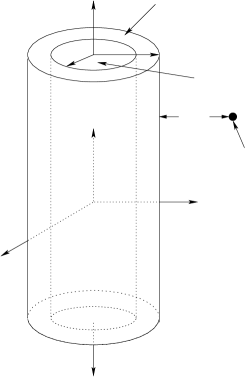
Figure 1: The geometry we are considering is a $2$-layer cylinder surrounded by an unbounded homogeneous medium. The outer region is labelled layer $3$ (vacuum), the coating is layer $2$ and the cylinder core is layer $1$. The distance from the surface of the outermost layer to the atom is $r$.

Because the Helmholtz equation is linear, the associated Green tensor can be written as a sum,

$$\bm{G}({\bf r},{\bf r}^{\prime},\omega)=\bm{G}^{0}({\bf r},{\bf r}^{\prime},\omega)+\bm{G}^{\text{wire}}({\bf r},{\bf r}^{\prime},\omega)\,,$$ (22)

where $\bm{G}^{0}({\bf r},{\bf r}^{\prime},\omega)$ represents the contribution from the vacuum and $\bm{G}^{\text{wire}}({\bf r},{\bf r}^{\prime},\omega)$ describes the part due to the wire. When the atom is located in layer 3, the scattering contribution is chew_90

$${\bm{G}}^{\text{wire}}({\bf r},{\bf r}^{\prime},\omega)=\frac{i}{8\pi}\int_{-\infty}^{\infty}dh\sum_{n=0}^{\infty}\frac{2-\delta_{0n}}{\eta_{3}^{2}}\;\bm{{\cal R}}_{n}(h)\,,$$ (23)

where

$$\bm{{\cal R}}_{n}(h)=$$

$$R_{n}^{11}(h)\bigg{[}{\bf N}_{{}^{e}n}^{(1)}(h){\bf N}_{{}^{e}n}^{{}^{\prime}(1)}(-h)+{\bf N}_{{}_{o}n}^{(1)}(h){\bf N}_{{}_{o}n}^{{}^{\prime}(1)}(-h)\bigg{]}$$

$$+ R^{12}_{n}(h)\left(-\frac{\omega\varepsilon_{3}}{k_{3}}\right)$$

$$\times\bigg{[}\,{\bf N}_{{}^{e}n}^{(1)}(h){\bf M}_{{}_{o}n}^{{}^{\prime}(1)}(-h)-{\bf N}_{{}_{o}n}^{(1)}(h){\bf M}_{{}^{e}n}^{{}^{\prime}(1)}(-h)$$

$$+{\bf M}_{{}^{e}n}^{(1)}(h){\bf N}_{{}_{o}n}^{{}^{\prime}(1)}(-h)-{\bf M}_{{}_{o}n}^{(1)}(h){\bf N}_{{}^{e}n}^{{}^{\prime}(1)}(-h)\,\bigg{]}$$

$$+ R^{22}_{n}(h)\bigg{[}{\bf M}_{{}^{e}n}^{(1)}(h){\bf M}_{{}^{e}n}^{{}^{\prime}(1)}(-h)+{\bf M}_{{}_{o}n}^{(1)}(h){\bf M}_{{}_{o}n}^{{}^{\prime}(1)}(-h)\bigg{]}\,.$$

For simplicity, we have omitted the tensor product symbol $\otimes$ between the even and odd cylindrical vector functions defined by ${\bf M}_{{}^{e}_{o}n}(h)=\nabla\times[\psi_{{}^{e}_{o}n}(h){\bf z}]$ and ${\bf N}_{{}^{e}_{o}n}(h)=\nabla\times\nabla\times[\psi_{{}^{e}_{o}n}(h){\bf z}]/k_{3}$. The scalar eigenfunctions $\psi_{{}^{e}_{o}n}(h)$ satisfy the homogeneous scalar wave equation chew_90 . It follows from these definitions that

$$\nabla\times{\bf M}_{{}^{e}_{o}n}(h) = k_{3}{\bf N}_{{}^{e}_{o}n}(h)\;,$$ (25)

$$\nabla\times{\bf N}_{{}^{e}_{o}n}(h) = k_{3}{\bf M}_{{}^{e}_{o}n}(h)\,.$$ (26)

Explicitly,

$${\bf N}_{{}^{e}_{o}n}(h)=\frac{1}{k_{3}}\bigg{[}ih\frac{dZ_{n}(\eta_{3}\rho)}{d\rho}\begin{array}[]{rr}\cos\\ \sin\end{array}(n\phi){\bf e}_{\rho}$$ (34)

$$\mp ih\frac{n}{\rho}Z_{n}(\eta_{3}\rho)\begin{array}[]{rr}\sin\\ \cos\end{array}(n\phi){\bf e}_{\phi}+\eta_{3}^{2}Z_{n}(\eta_{3}\rho)\begin{array}[]{rr}\cos\\ \sin\end{array}(n\phi){\bf e}_{z}\bigg{]}e^{ihz}\,,$$

$${\bf M}_{{}^{e}_{o}n}(h)=\bigg{[}\mp\frac{n}{\rho}Z_{n}(\eta_{3}\rho)\begin{array}[]{rr}\sin\\ \cos\end{array}(n\phi){\bf e}_{\rho}$$ (40)

$$\;-\,\frac{dZ_{n}(\eta_{3}\rho)}{d\rho}\begin{array}[]{rr}\cos\\ \sin\end{array}(n\phi){\bf e}_{\phi}\bigg{]}e^{ihz}\,.$$

The primes in Eq. (IV) indicate the spherical coordinates $(\rho^{\prime},\phi^{\prime},z^{\prime})$. The superscript $(1)$ indicates that $Z_{n}$ should be replaced by the Hankel function of first kind $H_{n}^{(1)}$. Otherwise, $Z_{n}$ is the Bessel function of first kind $J_{n}$. The propagation constant in the $\rho$ direction is $\eta_{p}^{2}=k_{p}^{2}-h^{2}$, where $k_{p}$ is the wave number of the $p$th layer. The permittivity of the $p$th layer is denoted by $\varepsilon_{p}$. The scattering reflection coefficients $R^{kl}_{n}(h)$ are given in Appendix A ($k,l=1,2$).

The double curl of the Green tensor in Eq. (23) can be written

$$\nabla\times\nabla^{\prime}\times{\bf G}^{\text{wire}}({\bf r},{\bf r}^{\prime},\omega)=$$ (41)

$$\frac{i}{8\pi}\sum_{n=0}^{\infty}(2-\delta_{0n})\left[\begin{array}[]{rrr}(I_{n})_{xx}&(I_{n})_{xy}&(I_{n})_{xz}\\ (I_{n})_{yx}&(I_{n})_{yy}&(I_{n})_{yz}\\ (I_{n})_{zx}&(I_{n})_{zy}&(I_{n})_{zz}\end{array}\right],$$ (45)

where

$${\bf I}_{n}\equiv{\bf I}_{n}({\bf r},{\bf r}^{\prime},\omega)=\int_{-\infty}^{\infty}dh\;\frac{1}{\eta_{3}^{2}}\;\nabla\times\nabla^{\prime}\times\bm{{\cal R}}_{n}(h)\;.$$ (46)

Note that the curls are computed by replacing ${\bf N}_{{}^{e}_{o}n}(h)$ by ${\bf M}_{{}^{e}_{o}n}(h)$ and vice versa, according to Eqs. (25) and (26). Also note that the integration variable $h$ is the wave number in the $z$-direction (see Fig. 1). From the symmetry of the integrand, it is easy to show that $(I_{n}^{\text{lim}})_{xz}=(I_{n}^{\text{lim}})_{zx}=(I_{n}^{\text{lim}})_{yz}=(I_{n}^{\text{lim}})_{zy}=0$, where $(I_{n}^{\text{lim}})_{ij}\equiv\lim_{{\bf r}\rightarrow{\bf r}^{\prime}}$ $(I_{n}({\bf r},{\bf r}^{\prime},\omega))_{ij}$ ($i,j=x,y,z$). Note that the (Onsager) reciprocity relation as mentioned in Section II implies that $(I_{n}^{\text{lim}})_{ij}=(I_{n}^{\text{lim}})_{ji}$.

V The spin flip rate outside a $2$-layer wire

The spin-flip rate in free space is readily derived from Eq. (20) since $\mbox{Im}[\nabla\times\nabla\times$ $\bm{G}^{0}({\bf r}_{A},{\bf r}_{A},\omega_{if})]_{qp}$ $=(k_{3}^{3}/6\pi)\,\delta_{qp}$, where $k_{3}=\omega/c$ is the free space wave number corresponding to the atomic transition. We use the notation $k_{3}$ here because in our discussion of the cylindrical wire, the third layer is a vacuum. Hence

$$\Gamma^{\;0}_{if}=\,\mu_{0}\,\frac{(\mu_{B}g_{S})^{2}}{3\pi\,\hbar}\,k_{3}^{3}S_{if}^{\,2}\;,$$ (47)

where we have introduced the angular factor $S_{if}^{\,2}\equiv|\langle i|\hat{S}_{x}|f\rangle|^{2}$ $+|\langle i|\hat{S}_{y}|f\rangle|^{2}$ $=2\,|\langle i|\hat{S}_{x}|f\rangle|^{2}$. We do not have a term containing $\hat{S}_{z}$ since we are interested here in a spin flip, which by definition changes $m_{F}$. We have moreover used the fact that the two transverse matrix elements are equal in absolute value as a result of symmetry. For the ⁸⁷Rb ground state transition $|F,m_{F}\rangle=|2,2\rangle\rightarrow|2,1\rangle$, the angular factor $S_{21}^{\,2}=1/8$ .

In order to find the contribution of the wire to the spontaneous spin-flip rate, we use Eqs. (20) and (41). The quantization axis is taken to be along the $z$ direction, corresponding to the direction of the bias field that the trapped atoms experience in the experiment. We obtain

$$\Gamma^{\text{wire}}_{if}=\frac{3}{8}\,\Gamma^{\;0}_{if}\sum_{n=0}^{\infty}(2-\delta_{0n})\textrm{Re}\left[(\widetilde{I}_{n}^{\text{\text{lim}}})_{xx}+(\widetilde{I}_{n}^{\text{lim}})_{yy}\right]\,.$$ (48)

Here we have once again used the facts that $|\langle i|\hat{S}_{x}|f\rangle|^{2}=|\langle i|\hat{S}_{y}|f\rangle|^{2}$ and that $\langle i|\hat{S}_{z}|f\rangle=0$. The dimensionless integrals $(\widetilde{I}_{n}^{\text{lim}})_{ij}\equiv(I_{n}^{\text{lim}})_{ij}/k_{3}^{3}$ are given by

$$(\widetilde{I}_{n}^{\text{lim}})_{xx}+(\widetilde{I}_{n}^{\text{lim}})_{yy}=\int_{-\infty}^{\infty}dq\;\frac{1}{\widetilde{\eta}_{3}^{2}}\times$$ (49)

$$\bigg{\{}\,[\,R_{n}^{11}(q)+q^{2}\,R_{n}^{22}(q)\,][\,(H_{n3})^{2}\frac{n^{2}}{k_{3}^{2}(a_{2}+r)^{2}}+(\widetilde{\eta}_{3}H_{n3}^{\prime})^{2}\,]$$

$$+2iqR_{n}^{12}(q)\left(-\frac{\omega\varepsilon_{3}}{k_{3}}\right)\;\widetilde{\eta}_{3}(H_{n3}^{2})^{\prime}\frac{n}{k_{3}(a_{2}+r)}\bigg{\}},$$

since $\rho=a_{2}+r$. We have used the simplified notation $Z_{np}\equiv Z_{n}(\widetilde{\eta}_{p}k_{3}\rho)$ and the primes in Eq. (49) denote the derivative with respect to the full argument of the relevant function, e.g. $Z_{np}^{\prime}\equiv dZ_{n}(\widetilde{\eta}_{p}k_{3}\rho)/d(\widetilde{\eta}_{p}k_{3}\rho)$. We have also chosen to write the permittivity of the $p$th layer relative to the outermost layer, i.e. $\varepsilon_{p}=\varepsilon_{3}\varepsilon_{p}^{\text{rel}}$. The wave number for layer $p$ is then given by $k_{p}^{2}=k_{3}^{2}\varepsilon_{p}^{\text{rel}}$, and the dimensionless propagation constant $\widetilde{\eta}_{p}\equiv\eta_{p}/k_{3}$ in the $\rho$ direction can be written as $\widetilde{\eta}_{p}=\sqrt{\varepsilon_{p}^{\text{rel}}-q^{2}}$, where $q\equiv h/k_{3}$ is the dimensionless integration variable.

The skin depth is the characteristic length scale on which an electromagnetic wave is damped within a conducting medium. It is given by $\delta_{p}=\sqrt{2\varepsilon_{0}\rho_{p}\omega}/k_{0}$ (see e.g. Ref. Jackson_75 ), where $\rho_{p}$ is the resistivity of layer $p$. Since the spin-flip frequency is very much lower than the resonance frequencies of the material in the wire, the relative permittivity is related to the skin depth by Jackson_75

$$\varepsilon_{p}^{\text{rel}}\approx\frac{i}{\varepsilon_{0}\rho_{p}\omega}=i\frac{2}{k_{0}^{2}\delta^{2}_{p}}\;.$$ (50)

We see from Eq. (22) that the total spin-flip rate is equal to the sum of the free space contribution and the scattering contribution. The total spin-flip rate for the rate-limiting transition $|2,2\rangle\rightarrow|2,1\rangle$ is therefore

$$\Gamma^{B}_{21}=\,\big{(}\Gamma^{\;0}_{21}+\Gamma^{\text{wire}}_{21}\,\big{)}\,(\overline{n}_{\text{th}}+1)\;.$$ (51)

VI Numerical results

In the experiment of Ref.hinds_03 , cold atoms are held in a microscopic trap near a current-carrying wire assumed to be at room temperature. The lifetime for atoms to remain in the microtrap is measured over a range of distances down to $27\,\mu$m from the surface of the wire. The wire consists of a central copper core with radius $a_{1}=185\,\mu$m and a $55\,\mu$m thick aluminium layer, i.e. $a_{2}=240\,\mu$m. Using Eq. (50), the resistivities $\rho_{1}=1.6\cdot 10^{-8}\,\Omega$m for Cu and $\rho_{2}=2.7\cdot 10^{-8}\,\Omega$m for Al give skin depths of $\delta_{1}=85\,\mu$m for Cu and $\delta_{2}=110\,\mu$m for Al at frequency $f=\omega/2\pi=560$ kHz.

Figure 2: Lifetime $\tau$ of the trapped atom as a function of the atom-surface distance $r$. Dotted curve: calculated spin-flip lifetime near a $2$-layer wire at $300\,$K with the parameters $f=560\,$kHz, $a_{1}=185\,\mu$m, $a_{2}=240\,\mu$m, $\delta_{1}=85\,\mu$m, and $\delta_{2}=110\,\mu$m. Solid curve: The same but at $380\,$K. Dot-dashed curve: calculated lifetime near a thick Al slab at $380\,$K with $\delta=110\,\mu$m (using Eq. (35) of Ref. henkel_99 ). Crosses: measured lifetimes of Ref. hinds_03 .

The dotted line in Fig. 2 shows the lifetime $\tau=1/\Gamma^{B}_{21}$ that we have calculated assuming a temperature of $300\,$K, together with the measured lifetimes (crosses). We see that the experimental results are close to the theory, indicating that the thermal spin flip mechanism is the primary cause of atom loss in the experiment. Nevertheless there is also a clear systematic discrepancy, with the measured lifetimes being $20-30\%$ shorter than expected. We find excellent agreement when the temperature in our theory is increased to $380\,$K, as shown by the solid curve in Fig. 2. We have re-examined the conditions under which the experiment was run and consider it most likely that the wire temperature was indeed $\sim 380\,$K, rather than the $300\,$K previously assumed. Such a temperature rise would be consistent with known power dissipation and with reasonable assumptions about the heat flow. In effect, the thermally driven spin flips have allowed us to measure the temperature of the wire!

The theory for the decay rate of an atom above a plane, thick slab is already known henkel_99 . Applying this theory to an Al slab with skin depth $\delta=110\,\mu$m and temperature $380\,$K, we obtain the result shown dot-dashed in Fig. 2. This curve lies below that for the wire, simply reflecting the fact that the slab contains a larger volume of fluctuating polarization than the wire. Naturally, the two $380\,$K curves converge at sufficiently small atom-surface distances ($r\ll\delta_{2}$, $\delta_{1}$, $a_{2}$), and in that range they vary linearly with distance henkel_99 .

Figure 3: Lifetime $\tau$ of the trapped atom as a function of the skin depth $\delta_{2}$ of the outer layer. The atom-surface distance is fixed at $r=50\,\mu$m. The other parameters are: $f=560$ kHz, $T=300$ K, $a_{1}=185\,\mu$m, $a_{2}=240\,\mu$m, and $\delta_{1}=85\,\mu$m. The straight dashed line represents the large $\delta_{2}$ limit. The numerical value for this limit is $52\,$s.

The lifetime for the atom to remain in the trap exhibits a minimum with respect to variation of the skin depth, as illustrated in Fig. 3, where the skin depth of the wire core $\delta_{1}$ is fixed at $85\mu$m but the skin depth of the outer layer $\delta_{2}$ is varied. Below the minimum at $\delta_{2}\simeq 20\,\mu$m, a decrease of skin depth leads to an increase of lifetime in proportion to $\delta_{2}^{-1}$. This happens despite a growth in the polarization noise [see Eqs. (6) and (50)] because the region generating the noise is becoming thinner. In the small $\delta_{2}$ limit the outer layer approaches a perfect conductor, the core wire does not play any role, and the lifetime becomes exceedingly long. By contrast, when the skin depth increases above $20\,\mu$m, the reduction in polarization noise is more influential than the growth of the source volume. In this region it is the worse conductor that gives the longer lifetime. At large $\delta_{2}$, the outer layer of the wire approaches the free space limit, and the lifetime is entirely determined by the skin depth and radius of the core. From a practical viewpoint it would normally be desirable to avoid the minimum of the lifetime curve. This means avoiding surface materials whose skin depth at the spin flip frequency is comparable with the atom-surface distance. This is a generic result. For example, at height z above a slab, one obtains the shortest lifetime when the skin depth is $z/3^{1/3}$, as is readily derived from equation (23) of Ref. henkel_99 .

Figure 4: Lifetime $\tau$ as a function of atom-surface distance $r$, with $r$, $a_{1}$ and $a_{2}$ scaling together according to $a_{2}=5r$ and $a_{1}=(185/240)a_{2}$. The other parameters are: $f=560$ kHz, $T=300$ K, $\delta_{1}=85\,\mu$m, and $\delta_{2}=110\,\mu$m.

From the same perspective of cold atoms trapped above small integrated circuits (atom chips) it is also interesting to see how the lifetime is altered when the dimensions $a_{1}$, $a_{2}$ of the wire are varied or the atom-surface distance $r$ changes. For example, let us scale all three lengths together, such that $r=a_{2}/5$ and $a_{1}=(185/240)a_{2}$, while the skin depths are fixed. The result of such a scaling is illustrated in Fig. 4. When the atom-surface distance is large compared with the skin depth, i.e. $r=a_{2}/5\gg\delta_{2}\sim 100\,\mu$m, the spin-flip lifetime scales as $\sim r^{4}$. This has the same exponent as the $z^{4}$ scaling of lifetime that applies at distance $z$ from a slab in the range where $z\gg\delta$ henkel_99 . The correspondence seems natural to us since the wire is essentially a curved slab when the skin depth is small. For a given ratio of atom-surface distance to wire size, the two lifetimes should therefore be related by a constant geometrical factor, resulting in the same distance scaling. At the opposite extreme, where $z\ll\delta$, the slab result is $\tau\propto z$. By contrast, we see in Fig. 4 that the lifetime outside the wire approaches a constant when $a_{2}=5r\ll\delta_{2}$. This difference occurs because the thickness of the source region is not the skin depth, but rather the diameter of the wire, which we are scaling linearly with $r$. In a similar way, it is possible to lengthen the lifetime of an atom above a slab by reducing the thickness of the slab to less than the skin depth hinds_03 .

As a second example of scaling, we change the diameter of the wire, keeping $a_{1}=(185/240)a_{2}$ but fixing the distance from the surface at $50\,\mu$m. Once again the skin depths are fixed. The resulting variation in the lifetime of the atom with wire size is shown in Fig. 5. At large wire diameter, the lifetime approaches $8.2$ s, which is of course the same as the lifetime $50\,\mu$m above a slab with $110\,\mu$m skin depth. By contrast, when the wire size is small, i.e. $a_{2}\ll r,\delta_{2}$, the decreasing volume of material leads to a $a_{2}^{-3}$ scaling of the lifetime. In the limit $a_{2}\rightarrow 0$, $\Gamma^{\text{wire}}_{if}$ vanishes and the lifetime for the atoms to remain in the trap is just the free-space blackbody rate given by the first term in Eq. (51). For $f=560$ kHz and $T=300$ K, this free space lifetime is an astonishing $\sim 10^{18}$ s (see also Purcell ). This figure emphasizes the very low strength of the electromagnetic field fluctuations in free space compared with those near a dielectric medium due to the surface modes.

Figure 5: Lifetime $\tau$ as a function of outer wire radius $a_{2}$ with the atom-surface distance fixed at $r=50\mu$m. The inner radius is scaled according to $a_{1}=(185/240)a_{2}$. Other parameters are: $f=560$kHz, $T=300$K, $\delta_{1}=85\mu$m, and $\delta_{2}=110\mu$m. Dotted line: the large $a_{2}$ limit.

VII Conclusions

In this paper we have derived the magnetic spin flip rate for an atom close to an absorbing dielectric body. The rate is given in terms of a dyadic Green tensor, allowing the expression to be applied in principle to a dielectric body of any shape. We derive an explicit expression for the spin-flip rate of an atom outside a 2-layer cylindrical wire, as used in the experiment of Jones et al. hinds_03 . We compare our numerical results with their measurements and we find lifetimes marginally longer than those measured in the experiment. The most likely explanation for this discrepancy is that the wire was hotter than previously thought. We also compare the cylindrical case with that of a slab and show that the spin-flip lifetime is systematically longer above a cylinder, as one would expect.

We have investigated how the lifetime of the atoms depends on the skin depth of the material. We find the generic result that there is a minimum in the lifetime when the skin depth is comparable with the atom-surface distance. When the dimensions of the wire and the atom-surface distance $r$ are varied together, the lifetime scales as $r^{4}$ at large $r$, following the same scaling law as a corresponding plane, thick slab, whereas the lifetime approaches a constant at small $r$. If instead we fix the atom-surface distance and vary only the dimensions of the wire, the lifetime scales as $r^{-3}$ when the wire is small, leaving only the very weak free-space decay rate in the limit of a vanishing wire diameter. The main conclusion for atom chip design is that one should avoid a material whose skin depth at the spin flip transition frequency is comparable with the atom-surface distance. The lifetime can also be improved by making sure that metal films on the surface are thinner than the skin depth.

Appendix A The scattering reflection coefficients

The scattering reflection coefficients for a cylindrical geometry can be computed for any number of layers (see e.g. Refs. chew_90 ; xiang_96 ; li_00 ; tai_93 ). In this Appendix we present the explicit expressions for the scattering reflection coefficients corresponding to our $3$-layer cylindrical geometry. To find these reflection coefficients we have used the iteration tensor equations in Ref. chew_90 . These iteration equations are given for arbitrary complex permittivity $\varepsilon_{p}$ and arbitrary complex permeability $\mu_{p}$. Therefore, the reflection coefficients presented in this Appendix apply to arbitrary $\varepsilon_{p}$ and arbitrary $\mu_{p}$. However, we stress that the theory presented in the main body of this paper is particular to non-magnetic media; we assume that $\mu_{p}=\mu_{0}$ in all the layers $p$.

The reflection coefficients are given as follows:

$$R_{n}^{11}(h) = \frac{(-1)}{d_{n32}}\left[a^{H_{3}^{\prime}J_{2}}_{n\mu_{3}}a^{J_{3}^{\prime}J_{2}}_{n\varepsilon_{3}}+b^{H_{3}J_{2}}_{n}b^{J_{3}J_{2}}_{n}\right]$$ (52)

$$+ \bigg{(}\frac{2\omega}{\pi a_{2}}\bigg{)}^{2}\eta_{3}^{2}\eta_{2}^{2}\varepsilon_{3}\frac{T_{n}^{11}}{N_{n}}\,,$$

$$R_{n}^{12}(h) = \frac{1}{d_{n32}}\left[a^{H_{3}^{\prime}J_{2}}_{n\mu_{3}}b^{J_{3}J_{2}}_{n}-a^{J_{3}^{\prime}J_{2}}_{n\mu_{3}}b^{H_{3}J_{2}}_{n}\right]$$ (53)

$$+ \bigg{(}\frac{2\omega}{\pi a_{2}}\bigg{)}^{2}\eta_{3}^{2}\eta_{2}^{2}\mu_{3}\frac{T_{n}}{N_{n}}\,,$$

where

$$T_{n}^{11} = d_{n32}\alpha_{n}-t_{n21}\beta_{n}\,,$$ (54)

$$T_{n}\; = d_{n32}\gamma_{n}-t_{n21}\delta_{n}\,,$$ (55)

and

$$N_{n} = (d_{n32})^{2}\bigg{[}\,d_{n32}d_{n21}+t_{n21}t_{n32}$$ (56)

$$- (a_{11}b_{11}-2\frac{\varepsilon_{2}}{\mu_{2}}a_{12}b_{12}+a_{22}b_{22})\,\bigg{]}\,.$$

Moreover, we have

$$\alpha_{n} = -(a^{H_{3}^{\prime}J_{2}}_{n\mu_{3}})^{2}\varepsilon_{2}b_{11}+(b^{H_{3}J_{2}}_{n})^{2}\mu_{2}b_{22}$$ (57)

$$-2\varepsilon_{2}b_{12}a^{H_{3}^{\prime}J_{2}}_{n\mu_{3}}b^{H_{3}J_{2}}_{n}\,,$$

$$\beta_{n} = -(a^{H_{3}^{\prime}J_{2}}_{n\mu_{3}})^{2}\varepsilon_{2}a_{22}+(b^{H_{3}J_{2}}_{n})^{2}\mu_{2}a_{11}$$ (58)

$$+2\varepsilon_{2}a_{12}a^{H_{3}^{\prime}J_{2}}_{n\mu_{3}}b^{H_{3}J_{2}}_{n}\,,$$

$$\gamma_{n} = -a^{H_{3}^{\prime}J_{2}}_{n\mu_{3}}b^{H_{3}^{\prime}J_{2}}_{n}\varepsilon_{3}b_{11}-a^{H_{3}^{\prime}J_{2}}_{n\varepsilon_{3}}b^{H_{3}J_{2}}_{n}\mu_{2}b_{22}$$ (59)

$$+\varepsilon_{2}b_{12}[a^{H_{3}^{\prime}J_{2}}_{n\mu_{3}}a^{H_{3}^{\prime}J_{2}}_{n\varepsilon_{3}}-(b^{H_{3}J_{2}}_{n})^{2}]\,,$$

$$\delta_{n} = -a^{H_{3}^{\prime}J_{2}}_{n\mu_{3}}b^{H_{3}J_{2}}_{n\varepsilon}a_{22}-a^{H_{3}^{\prime}J_{2}}_{n\varepsilon_{3}}b^{H_{3}J_{2}}_{n}\mu_{2}a_{11}$$ (60)

$$-\varepsilon_{2}a_{12}[a^{H_{3}^{\prime}J_{2}}_{n\mu_{3}}a^{H_{3}^{\prime}J_{2}}_{n\varepsilon_{3}}-(b^{H_{3}J_{2}}_{n})^{2}]\,,$$

and

$$a_{11} = a^{H_{3}^{\prime}J_{2}}_{n\mu_{3}}a^{H_{3}^{\prime}H_{2}}_{n\varepsilon_{3}}+b^{H_{3}J_{2}}_{n}b^{H_{3}H_{2}}_{n}\,,$$ (61)

$$a_{12} = a^{H_{3}^{\prime}J_{2}}_{n\mu_{3}}b^{H_{3}H_{2}}_{n}-a^{H_{3}^{\prime}H_{2}}_{n\mu_{3}}b^{H_{3}J_{2}}_{n}$$ (62)

$$= -\frac{2\omega}{\pi a_{2}}\eta_{3}^{2}\frac{hn}{a_{2}}\mu_{2}(H_{n3})^{2}\big{(}k_{2}^{2}-k_{3}^{2}\big{)}\,,$$

$$b_{11} = a^{H_{2}^{\prime}J_{1}}_{n\mu_{2}}a^{J_{2}^{\prime}J_{1}}_{n\varepsilon_{2}}+b^{H_{2}J_{1}}_{n}b^{J_{2}J_{1}}_{n}\,,$$ (63)

$$b_{12} = a^{H_{2}^{\prime}J_{1}}_{n\mu_{2}}b^{J_{2}J_{1}}_{n}-a^{J_{2}^{\prime}J_{1}}_{n\mu_{2}}b^{H_{2}J_{1}}_{n}$$ (64)

$$= -\frac{2\omega}{\pi a_{1}}\eta_{1}^{2}\frac{hn}{a_{1}}\mu_{2}(J_{n1})^{2}\big{(}k_{1}^{2}-k_{2}^{2}\big{)}\,.$$

The function $a_{21}$, $a_{22}$, and $b_{21}$, $b_{22}$ are obtained from $a_{12}$, $a_{11}$, and $b_{12}$, $b_{11}$, respectively, by replacing $\mu_{p}\leftrightarrow-\varepsilon_{p}$. In the last step in Eqs. (62) and (64) we have used the Wronskian determinant between Bessel and Hankel functions. Finally, we have

$$t_{n21} = a^{J_{2}^{\prime}J_{1}}_{n\mu_{2}}a^{J_{2}^{\prime}J_{1}}_{n\varepsilon_{2}}+(b^{J_{2}J_{1}}_{n})^{2},$$ (65)

$$t_{n32} = a^{H_{3}^{\prime}H_{2}}_{n\varepsilon_{3}}a^{H_{3}^{\prime}H_{2}}_{n\mu_{3}}+(b^{H_{3}H_{2}}_{n})^{2}\,,$$ (66)

$$d_{n21} = a^{H_{2}^{\prime}J_{1}}_{n\mu_{2}}a^{H_{2}^{\prime}J_{1}}_{n\varepsilon_{2}}+\big{(}b^{H_{2}J_{1}}_{n}\big{)}^{2}\,,$$ (67)

$$d_{n32} = a^{H_{3}^{\prime}J_{2}}_{n\mu_{3}}a^{H_{3}^{\prime}J_{2}}_{n\varepsilon_{3}}+\big{(}b^{H_{3}J_{2}}_{n}\big{)}^{2},$$ (68)

and

$$a^{H_{2}^{\prime}J_{1}}_{n\mu_{2}} = i\omega\eta_{2}\eta_{1}\left(\mu_{2}\eta_{1}H^{\prime}_{n2}J_{n1}-\mu_{1}\eta_{2}H_{n2}J^{\prime}_{n1}\right),$$ (69)

$$a^{J_{2}^{\prime}J_{1}}_{n\mu_{2}} = i\omega\eta_{2}\eta_{1}\left(\mu_{2}\eta_{1}J^{\prime}_{n2}J_{n1}-\mu_{1}\eta_{2}J_{n2}J^{\prime}_{n1}\right)\,,$$ (70)

$$a_{n\varepsilon_{2}}^{H_{2}^{\prime}J_{1}} = i\omega\eta_{2}\eta_{1}\left(\varepsilon_{2}\eta_{1}H^{\prime}_{n2}J_{n1}-\varepsilon_{1}\eta_{2}H_{n2}J^{\prime}_{n1}\right)\,,$$ (71)

$$a_{n\varepsilon_{2}}^{J_{2}^{\prime}J_{1}} = i\omega\eta_{2}\eta_{1}\left(\varepsilon_{2}\eta_{1}J^{\prime}_{n2}J_{n1}-\varepsilon_{1}\eta_{2}J_{n2}J^{\prime}_{n1}\right)\,,$$ (72)

$$b_{n}^{H_{2}J_{1}} = \frac{hn}{a_{1}}H_{n2}J_{n1}\left(k_{1}^{2}-k_{2}^{2}\right).$$ (73)

Whenever the combination $Z_{2}$ and $Z_{1}$ is involved in the superscript, the radius $a_{1}$ is implicit in the cylindrical functions. For example, in Eqs. (69)–(73) we have

$$Z_{n1}\equiv Z_{n}(\eta_{1}a_{1})\,,Z_{n2}\equiv Z_{n}(\eta_{2}a_{1})\,,$$ (74)

$$Z^{\prime}_{n1}\equiv\frac{dZ_{n}(\eta_{1}a_{1})}{d(\eta_{1}a_{1})}\,,\quad Z^{\prime}_{n2}\equiv\frac{dZ_{n}(\eta_{2}a_{1})}{d(\eta_{2}a_{1})}\,.$$ (75)

The functions $a^{H_{3}^{\prime}J_{2}}_{n\mu_{3}}$, $a^{J_{3}^{\prime}J_{2}}_{n\mu_{3}}$, $a_{n\varepsilon_{3}}^{H_{3}^{\prime}J_{2}}$, $a_{n\varepsilon_{3}}^{H_{3}^{\prime}H_{2}}$, $a_{n\varepsilon_{3}}^{J_{3}^{\prime}J_{2}}$, $b_{n}^{H_{3}J_{2}}$, and $b_{n}^{H_{3}H_{2}}$ are defined analogously, where we understand that the radius $a_{2}$ is implicit in all those functions. Of course, for the special case $\mu_{p}=1$ for all layers $p$, these reflection coefficients simplify.

The reflection coefficients $R_{n}^{21}(h)$ and $R_{n}^{22}(h)$ can be obtained from $R_{n}^{12}(h)$ and $R_{n}^{11}(h)$, respectively, by replacing $\mu_{p}\leftrightarrow-\varepsilon_{p}$. Note that the scattering coefficients $R_{n}^{11}(h)$ as well as $R_{n}^{22}(h)$ are dimensionless. However, the coefficients $R_{n}^{12}(h)$ and $R_{n}^{21}(h)$ are not, but the particular combinations $R_{n}^{12}(h)(-\omega\varepsilon_{3}/k_{3})=R_{n}^{21}(h)(\omega\mu_{3}/k_{3})$ are.

References

• (1) E.A. Hinds and I.A. Hughes, J. Phys. D: Appl. Phys. 32, R119 (1999); R. Folman, P. Krüger, J. Schmiedmayer, J. Denschlag, and C. Henkel, Adv. At. Mol. Opt. Phys. 48, 263 (2002).
• (2) T. Calarco, E.A. Hinds, D. Jaksch, J. Schmiedmayer, J.I. Cirac, and P. Zoller, Phys. Rev. A. 61, 022304 (2000).
• (3) J.B. Johnson, Phys. Rev. 32, 97 (1928); H. Nyquist, Phys. Rev. 32, 110 (1928).
• (4) M.P.A. Jones, C.J. Vale, D. Sahagun, B.V. Hall, and E.A. Hinds, Phys. Rev. Lett. 91, 080401 (2003).
• (5) D.M. Harber, J.M. McGuirk, J.M. Obrecht, and E.A. Cornell, J. Low. Temp. Phys. 133, 229-238 (2003).
• (6) C. Henkel, S. Pötting and M. Wilkens, Appl. Phys. B 69, 379 (1999); C. Henkel and M. Wilkens, Europhys. Lett. 47, 414 (1999).
• (7) L. Knöll, S. Scheel, and D.-G. Welsch, QED in dispersing and absorbing media, in Coherence and Statistics of Photons and Atoms, ed. J. Peřina (Wiley, New York, 2001); S. Scheel, L. Knöll, D.-G. Welsch, and S.M. Barnett, Phys. Rev. A 60, 1590 (1999); S. Scheel, L. Knöll and D.-G. Welsch, Phys. Rev. A 60, 4094 (1999); Ho Trung Dung, L. Knöll and D.-G. Welsch, Phys. Rev. A 62, 053804 (2000).
• (8) G.S. Agarwal, Phys. Rev. A 11, 230 (1975); J.M. Wylie and J.E. Sipe, Phys. Rev. A 30, 1185 (1984).
• (9) L.D. Landau and E.M. Lifshitz, Electrodynamics of continuous media (Pergamon Press, Oxford, 1960).
• (10) L. Onsager, Phys. Rev. 37, 405 (1931); 38, 2265 (1931);
• (11) W. Eckhardt, Opt. Commun. 41, 305 (1982); Phys. Rev. A 29, 1991 (1984).
• (12) W.C. Chew, Waves and Fields in Inhomogeneous Media (IEEE Press, New York, 1990).
• (13) J.D. Jackson, Classical Electrodynamics, 2nd edn. (Wiley, New York, 1975).
• (14) E.M. Purcell, Phys. Rev. 69, 681 (1946).
• (15) C.-T. Tai, Dyadic Green Functions in Electromagnetic Theory (IEEE Press, New York, 1993).
• (16) Z. Xiang and Y. Lu, IEEE Trans. Microwave Theory Tech. 44, 614 (1996).
As pointed out in Ref. li_00 , this paper contains some critical mistakes. The relation between the scattering coefficients and the Green tensor in this paper is inconsistent.
• (17) L.-W. Li, M.-S. Leong, T.-S. Yeo, and P.-S. Kooi, J. of Electromagnetic Waves and Appl. 14, 961 (2001).