Examples of nonuniform limiting distributions for the quantum walk on even cycles

Abstract

In the note we show how the choice of the initial states can influence the evolution of time-averaged probability distribution of the quantum walk on even cycles.

The analysis of discrete quantum random walks initiated by Aharonov et al. Aharonov et al. and its possible applications for constructing efficient quantum algorithms (Shenvi et al. -Ambainis et al. ) has recently attracted a lot of attention. Although many questions in this area remain open, it is well known that the behaviour of classical and quantum walks can be very different, as it can be seen by studying spreading, mixing and hitting times (Aharonov et al. , Ambainis et al. and Kempe (b)) or limiting distributions Bednarska et al. . One of the differences between quantum and classical walks we explore in this note is that one can start a quantum walk not from a single occupied node, but from the superposition of many nodes. The influence of the initial state on the behaviour of a quantum walk was studied by Tragenna et al. Tragenna et al. . In Bednarska et al. we mentioned the possibility of generating highly nonuniform limiting distributions in a quantum walk on even cycles starting from superposition states. In this note we show that the initial conditions can affect the time evolution of the total variation distance of time-averaged probability distribution in a decisive way.

We shall study a quantum random walk on an even cycle with $d$ nodes, using a model proposed by Aharonov et al. Aharonov et al. . In this setting the nodes of the cycle are represented by vectors $|v\rangle$, $v=0,1,\dots,d-1$, which form an orthonormal basis of the Hilbert space $H_{V}$. An auxiliary two-dimensional Hilbert space $H_{A}$ (coin space) is spanned by vectors $|s\rangle$, $s=0,1$. The initial state of the walk is a normalized vector

$$|\Psi_{0}\rangle=\sum_{s,v}\gamma_{sv}|s,v\rangle=\sum_{s,v}\gamma_{sv}|s\rangle|v\rangle$$ (1)

from the tensor product $H=H_{A}\otimes H_{V}$. In a single step of the walk the state changes according to the equation

$$|\Psi_{t+1}\rangle=U|\Psi_{t}\rangle,$$ (2)

where the operation $U=S(H\otimes I)$ first applies the Hadamard gate operator $H=\frac{1}{\sqrt{2}}\sum_{s,s^{\prime}}(-1)^{ss^{\prime}}|s\rangle\langle s^{\prime}|$ to the vector from $H_{A}$, and then shifts the state by the operator

$$S=\sum_{s,v}|s\rangle\langle s|\otimes|v+2s-1({\rm mod}\ d)\rangle\langle v|\,.$$ (3)

The operator $U$ has been studied in Bednarska et al. , where we prove that

$$U|\phi_{jk}\rangle=c_{jk}|\phi_{jk}\rangle,$$ (4)

where the eigenvalues $c_{jk}$ are given by

$$c_{jk}=\frac{1}{\sqrt{2}}\big{(}(-1)^{k}\sqrt{1+\cos^{2}(2\pi j/d)}-i\sin(2\pi j/d)\big{)},$$ (5)

for $k=0,1$, and $j=0,1,\dots,d-1$, while the corresponding eigenvectors are

$$|\phi_{jk}\rangle=(a_{jk}|0\rangle+a_{jk}b_{jk}|1\rangle)\otimes\sum_{v}\omega_{d}^{jv}|v\rangle,$$ (6)

where $\omega_{d}=e^{2\pi i/d}$,

$$a_{jk} =1\Big{/}\sqrt{d(1+|b_{jk}|^{2})},$$ (7)

$$b_{jk} =\omega_{d}^{j}\big{(}(-1)^{k}\sqrt{1+\cos^{2}(2\pi j/d)}-\cos(2\pi j/d)\big{)}.$$ (8)

The probability distribution on the nodes of the cycle after the first $t$ steps of the walk is given by

$$p_{t}(v)=\sum_{s}|\langle s,v|\Psi_{t}\rangle|^{2}.$$ (9)

As was observed by Aharonov at el. Aharonov et al. , for a fixed $v$, the probability $p_{t}(v)$ is ‘quasi-periodic’ as a function of $t$ and thus, typically, it does not converge to a limit. Thus, instead of $p_{t}(v)$, the authors of Aharonov et al. propose to consider time-averaged probability distribution

$$\bar{p}_{t}(v)=\frac{1}{t+1}\sum_{i=0}^{t}p_{t}(v),$$ (10)

and its limiting distribution

$$\pi(v)=\lim_{t\to\infty}\bar{p}_{t}(v).$$ (11)

In order to present the global properties of the walk let us also define the total variation distance

$$\Delta_{t}=\frac{1}{2}\sum_{v=0}^{d-1}\Big{|}\bar{p}_{t}(v)-\frac{1}{d}\Big{|},$$ (12)

which measures how far is time - averaged probability distribution from uniform distribution. $\Delta_{t}$ tends to limit which will be denoted by $\Delta_{\infty}=\lim_{t\to\infty}\Delta_{t}$.

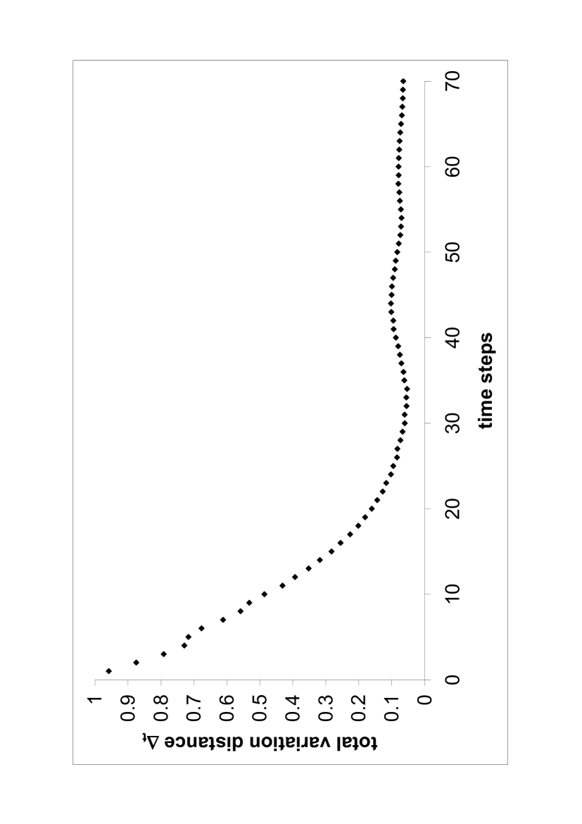
Figure 1: Time evolution of the total variation distance $\Delta_{t}$ for the initial state $|\Psi_{0}^{(2d)}\rangle$ ($d=24$).

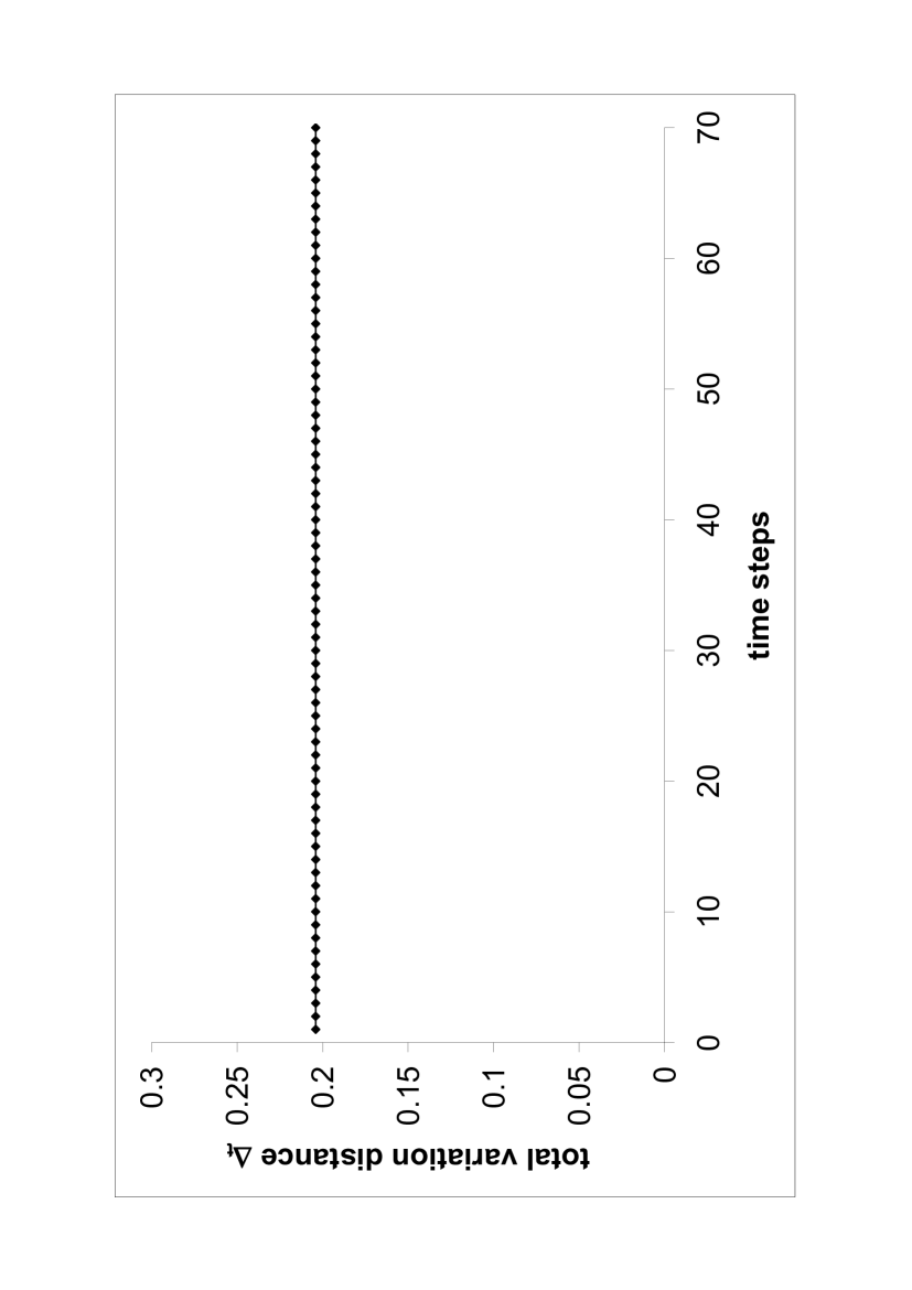
Figure 2: Time evolution of the total variation distance $\Delta_{t}$ for the initial state $|\Psi_{0}^{(2)}\rangle$ ($d=24$). Diamonds – numerical simulations, line – analytical value of Eq. (23).

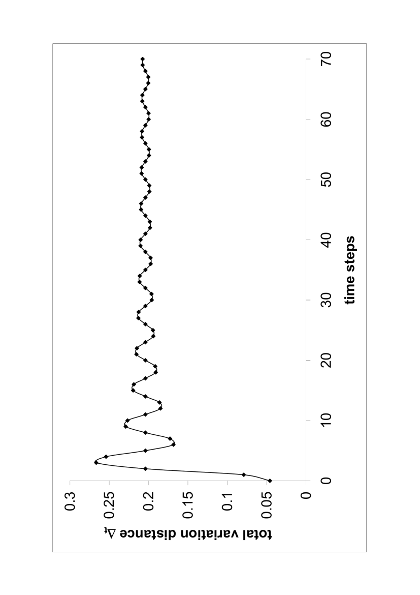
Figure 3: Time evolution of the total variation distance $\Delta_{t}$ for the initial state $|\Psi_{0}^{(4)}\rangle$ ($d=24$). Diamonds – numerical simulations, line – analytical value of Eqs. (12) and (26).

Figs. 1, 2, and 3, show the evolution of the total variation distance $\Delta_{t}$ for the case of three different initial states: $|\Psi_{0}^{(2d)}\rangle$, $|\Psi_{0}^{(2)}\rangle$ and $|\Psi_{0}^{(4)}\rangle$, which can be written as a superposition of some $2d$, $2$, and $4$, eigenvectors $|\phi_{jk}\rangle$, respectively. Thus, $|\Psi_{0}^{(2d)}\rangle=\sum_{jk}g_{jk}\omega_{d}^{-v_{0}j}|\phi_{jk}\rangle$ is the state with a single occupied node $v_{0}$ where $g_{jk}=a_{jk}(1+ib_{jk}^{\ast})/\sqrt{2}$; $|\Psi_{0}^{(2)}\rangle=\frac{1}{\sqrt{2}}\left(|\phi_{3,0}\rangle+|\phi_{9,0}\rangle\right)$ is a superposition of two degenerate eigenvectors; finally $|\Psi_{0}^{(4)}\rangle=\frac{1}{\sqrt{2}}\left(|\phi_{3,0}\rangle+|\phi_{9,0}\rangle-|\phi_{15,0}\rangle-|\phi_{21,0}\rangle\right)$.

In the case a quantum walk starts with $|\Psi_{0}^{(2d)}\rangle$, one observe decaying of the total variation distance to the nonzero value $\Delta_{\infty}^{(2d)}$ (Fig. 1). An analytic form of $\Delta_{\infty}^{(2d)}$ can be found in a similar way as in Bednarska et al. (we remark that there is a minor error in the equation (22) in Bednarska et al. ). Thus, we get

$$\pi(v)=\frac{1+f(s)-(-1)^{\xi}f(s^{\prime})}{d},$$ (13)

where

$$f(x)=\frac{\sqrt{2}}{1-(-z)^{d/2}}z^{x}-\delta_{x0}-\frac{1}{d},$$ (14)

$$\xi=\frac{(1+(-1)^{d/2})}{2},$$ (15)

(i.e., $\xi=1$ when $d/2$ is even, and $\xi=0$ if $d/2$ is odd), and

$$s=s(v)=\min\left(|v-v_{0}|,d-|v-v_{0}|\right),$$ (16)

denotes the distance between nodes $v_{0}$ and $v$, and $s^{\prime}=d/2-s$. If $d\gg 1$ we can write $\Delta_{\infty}^{2d}$ in a simple form. When $\xi=0$

$$\Delta_{\infty}^{(2d)}=1/d,$$ (17)

while in the case of $\xi=1$

$$\Delta_{\infty}^{(2d)}=\frac{2}{d}-\frac{4}{d^{2}}\left(1-2\frac{\log_{2}d-1/2}{\log_{2}z}\right),$$ (18)

where $z=3-2\sqrt{2}$. For the particular case presented at Fig. 1, (18) gives the value $\Delta_{\infty}^{(2d)}=0.054$. Hence, if we start with a single occupied node, the total variation distance decreases steadily in time and its limiting value tends to zero as the graph size $d$ grows. Let us present now two examples of walk for which the dynamics of the total variation distance is dramatically different. Fig. 2 pictures the evolution of a walk where $\Delta_{t}^{(2)}\neq 0$ does not change in time. It starts with the initial state of the form the form

$$\frac{1}{\sqrt{2}}\left(|\phi_{m,k}\rangle+|\phi_{d/2-m,k}\rangle\right),$$ (19)

for $m=3$ and $k=0$. The state described by (19) for $m=0,\dots,m_{\max}$ as well as the state

$$\frac{1}{\sqrt{2}}\left(|\phi_{d/2+m,k}\rangle+|\phi_{d-m,k}\rangle\right),$$ (20)

for $m=1,\dots,m_{\max}$, ($m_{\max}=\lfloor(d-2)/4\rfloor$) consists of two degenerated eigenvectors. Since the evolution of the superposition of any number of degenerated eigenvectors leads only to the global phase changes so the dynamics of the probability distribution is frozen and $\pi(v)=\bar{p}_{t}(v)=p_{0}(v)$. For the states given by (19) and (20) the limiting distribution takes form

$$\pi(v)=\frac{1}{d}+\frac{(-1)^{v}\sin\alpha}{d\sqrt{1+\cos^{2}\alpha}}\sin\left(\alpha\left(2v+1\right)\right),$$ (21)

where $\alpha=2\pi m/d$. Thus

$$\Delta_{t}^{(2)}=\frac{\sin\alpha}{d\sqrt{1+\cos^{2}\alpha}}\sum_{v}\big{|}\sin\left(\alpha\left(2v+1\right)\right)\big{|}.$$ (22)

When $m$ divides $d/2$ the summation can be easily perform leading to

$$\Delta_{t}^{(2)}=\frac{m}{d}\frac{1}{\sqrt{1+\cos^{2}\alpha}}\left(1-\cos\left(2\alpha\left(\eta+1\right)\right)\right),$$ (23)

where

$$\eta=\lfloor\frac{d}{4m}-\frac{1}{2}\rfloor.$$ (24)

For $m=3$ and $d=24$ (23) gives $0.204$.

The last example of the time evolution, depicted at Fig. 3, is, perhaps, most intriguing. The changes of the total variation distance in this case resembles the motion of the damped harmonic oscillator with shifted equilibrium. Let us emphasize also that the limiting value of the total variation distance $\Delta_{\infty}^{(4)}$ is much higher than the initial one $\Delta_{0}^{(4)}$. The initial state $|\phi_{0}^{(4)}\rangle$ is of the kind

$$\frac{1}{2}\left(|\phi_{m,k}\rangle+|\phi_{d/2-m,k}\rangle-|\phi_{d/2+m,k,k}\rangle-|\phi_{d-m,k}\rangle\right).$$ (25)

The time-averaged probability distribution for the initial states of the form given by (25) can be described as

$$\bar{p}_{t}(v)=A(v)+B(v)\frac{\sin\left(2\varphi_{mk}(t+1)\right)}{t+1},$$ (26)

where $A(v)=\pi(v)$, $B(v)=\left(p_{0}(v)-\pi(v)\right)/\sin(2\varphi_{mk})$, $\varphi_{mk}$ is the phase of the eigenvalue $c_{mk}$ $\left(c_{mk}=e^{i\varphi_{mk}}\right)$ and $\pi(v)$ is given by (21). Fig. 3 presents $\Delta_{t}^{(4)}$ calculated with the use of (12) and (26) as well as the results of numerical calculation.

In conclusion, we demonstrated how the initial conditions affects the dynamics of the quantum walk on cycle. We gave examples for three different kinds of behavior of the total variation distance between given distribution and uniform distribution: decaying, constant and damped oscillating.

References

(1)
D. Aharonov,
A. Ambainis,
J. Kempe, and
U. Vazirani,
Proceedings of the 30th Annual ACM Symposium on Theory of
Computation (ACM Press, New York, 2001)
50 (2001).
(2)
N. Shenvi,
J. Kempe, and
K. Whaley,
eprint quant-ph/0210064.
(5)
F. Magniez,
M. Santha,
M. Szegedy,
eprint quant-ph/0310134.
(6)
A. Ambainis,
J. Kempe,
A. Rivosh,
eprint quant-ph/0210064.
(7)
A. Ambainis,
E. Bach,
A. Nayak,
A. Vishwanath,
and J. Watrous,
Proceedings of the ACM Symposium on Theory of Computation
(ACM Press, New York, 2001)
37 (2001).
Kempe (b)
J. Kempe,
Proc. of 7th Intern. Workshop on Randomization and Approximation Techniques in Comp. Sc. (RANDOM’03)
354 (2003).
(9)
M. Bednarska,
A. Grudka,
P. Kurzyński,
T. Łuczak,
and A. Wójcik,
Phys. Lett. A 317,
21 (2003).
(10)
B. Tragenna,
W. Flanagan,
R. Maile,
V. Kendon,
New. J. Phys. 5,
83.1 (2003).