Quantum State Detector Design:
Optimal Worst-Case a posteriori Performance

Abstract

The problem addressed is to design a detector which is maximally sensitive to specific quantum states. Here we concentrate on quantum state detection using the worst-case a posteriori probability of detection as the design criterion. This objective is equivalent to asking the question: if the detector declares that a specific state is present, what is the probability of that state actually being present? We show that maximizing this worst-case probability (maximizing the smallest possible value of this probability) is a quasiconvex optimization over the matrices of the POVM (positive operator valued measure) which characterize the measurement apparatus. We also show that with a given POVM, the optimization is quasiconvex in the matrix which characterizes the Kraus operator sum representation (OSR) in a fixed basis. We use Lagrange Duality Theory to establish the optimality conditions for both deterministic and randomized detection. We also examine the special case of detecting a single pure state. Numerical aspects of using convex optimization for quantum state detection are also discussed.

1 Introduction

why

Information is extracted from a quantum system by measurement. The most information that it is possible to extract from the quantum system is given by its state, specified by a density operator, and it is impossible to determine this from a single measurement. The problem of detecting information stored in the state of a quantum system is therefore a fundamental problem in quantum information theory. The nature of this problem is essentially the design of measurements such that they yield the optimum information for the specified purpose. That is, the construction of matrices representing positive operator valued measures (POVMs) which give the best performance against a given set of criteria, subject to constraints reflecting the underlying properties of the quantum mechanics, or costs associated with the implementation of certain operations.

The emergence of quantum information processing has raised important new issues, and made more urgent the development of tools for the design of quantum measurements. In this paper we present a general formalism that enables this design across a wide range of applications. In particular we show that the problem may be cast in the form of a convex optimization over the possible POVMs, and that this allows powerful numerical tools to identify the globally optimal measurements to achieve the desired objective. Such optimizations are useful even if they turn out to be difficult to implement in the laboratory, since they provide a benchmark for the performance of experimentally feasible measurements.

The objective of a measurement in quantum information theory depends on the way in which information is encoded into the quantum system to begin with, and this is in turn, depends on the application. In quantum cryptography, for example, the information is encoded by the sender choosing randomly between two non-orthogonal bases, both of which can encode a single bit. The ability of an eavesdropper, who is in principle unable to influence the choice of preparation and measurement bases chosen by the sender and receiver of this information, to extract information from the transmitted quantum bits, depends on her ability to determine which of four non-orthogonal states were sent. In a quantum information processor, the information in the register at the end of a computation often resides in orthogonal states, and the goal of the measurement is simply to read out the register by distinguishing among the sets of such states. However, the operation of such a processor may itself depends on measurements. For example, quantum error correction protocols require the measurement of an ancilla to preserve the quantum state of the register itself. In another example, the cluster computing model [40] and the linear optical quantum computer [29], both rely on measurements of ancillary qubits for the operation of the logic gates themselves.

In these examples of conditional state preparation, it is vital that there is a high degree of correlation between the outcome of the measurement and the quantum state prepared in the register by the measurement. The structure of the measurement should therefore be such that this correlation is maximized. Thus it is vital to consider the case when the detectors have noise, and to develop strategies for optimizing the measurement in the presence of this and inherent inefficiencies. Despite the fundamental inability to determine the quantum state of a system from a single measurement, it is sometimes useful to make such a determination from a set of independent measurements on identically prepared systems. This procedure is called quantum state tomography. Similarly, one may characterize the action of a quantum operation by determining its effect on a known input quantum state from a determination of the output state. In this application, the central questions are: how many measurements are needed to determine the state to within a given precision, and how should these measurements be constructed? That is, it is essentially a problem of experiment design. Optimal experiment for quantum state tomography and quantum process tomography is considered in [30].

In this work, we concentrate on the problem of quantum state detection. That is, the design of POVMs that can determine whether or not a particular component was present in the input state to the detector. The problem is thus equivalent to the design of a quantum channel that optimally transforms the input state distribution (assumed to be given, and including non-orthogonal states) to the output measurement outcomes. The channel may be lossy, and may introduce noise, and thus there may be latency in the measurement, in which certain outcomes are ambiguous.

previous work

Several approaches have emerged for distinguishing between a collection of non-orthogonal quantum states. An accessible review can be found in the article by Chefles [8]. In one approach, called quantum hypothesis testing, a measurement is designed to minimize the probability of a detection error [25, 23, 44, 17, 6, 35, 2, 15, 16, 14]. Necessary and sufficient conditions for an optimum measurement maximizing the probability of correct detection have been developed in [17] using a semidefinite programming approach, and earlier in [25] (the drawback of this approach is that it does not readily lend itself to efficient computational algorithms). Closed-form analytical expressions for the optimal measurement have been derived for several special cases [23, 6, 35, 2, 15, 16]. Iterative procedures maximizing the probability of correct detection have also been developed for cases in which the optimal measurement cannot be found explicitly [24, 17]. A specific design for achieving the optimal discrimination between non-orthogonal coherent states has been given in [3], and for non-orthogonal polarization states of a single photon by [4]. Optimal discrimination amongst more than two non-orthogonal states has also been analyzed [39] and demonstrated experimentally [10].

A more recent approach, referred to as unambiguous detection [27, 11, 36, 28, 38, 7, 9, 13, 12, 18], is to design a measurement that with a certain probability returns an inconclusive result, but such that if the measurement returns an answer, then the answer is correct with probability $1$. Chefles [7] showed that a necessary and sufficient condition for the existence of unambiguous measurements for distinguishing between a collection of pure quantum states is that the states are linearly independent. Necessary and sufficient conditions on the optimal measurement minimizing the probability of an inconclusive result for pure states were derived in [13]. The optimal measurement when distinguishing between a broad class of symmetric pure-state sets was also considered in [13]. The problem of unambiguous detection between mixed state ensembles was first considered in [41]. Necessary and sufficient optimality conditions for unambiguous mixed state detection were developed in [18].

Experimental configurations may not allow the ideal measurements to be made, and thus the performance of feasible apparatuses have been analyzed. For example, an apparatus for the unambiguous discrimination between two orthogonal states of a single photon using homodyne detection, rather than photon counting, which has higher losses and more noise, has been examined in [22] and [33]. An experimental implementation of the process for discriminating unambiguously between two non-orthogonal states of polarization of a single photon has been demonstrated in [26].

An interesting alternative approach for distinguishing between a collection of quantum states, which is a combination of the previous two approaches, is to allow for a certain probability of an inconclusive result, and then maximize the probability of correct detection [12, 45, 20].

what’s new here

Prior work has considered optimal detector design only for an average measure of the probability of detection, such as the average joint probability of detection. For example, in [17, 13] it is shown that using this criterion, detector design can be formulated as a convex optimization over the matrices in the POVM, specifically a semidefinite program (SDP). Here we concentrate on quantum state detection using the worst-case a posteriori probability of detection as the design criterion. This objective is equivalent to asking the question: if the detector declares that a specific state is present, what is the probability of that state actually being present? We show that maximizing the smallest possible value of this probability is a quasiconvex optimization over the POVM matrices, or over the Krause operator-sum-representation (OSR) in a fixed basis. Issues relating to conditions of optimality and numerical aspects of convex optimization of state detection are also discussed.

We will show that many of the standard measures of detector performance (including those previously considered) are also convex functions of the detector design parameters. In addition, we will see that the design parameters, either POVM or OSR, are in a convex set. As a result we can cast a number of detector design problems as a convex optimization. Details and underlying theory about convex optimization are in the text by Boyd and Vandenberghe [5]. As stated there, the great advantage of convex optimization is a globally optimal solution can be found efficiently and reliably, and perhaps most importantly, can be computed to within any desired accuracy using an interior-point method.

Another advantage to being able to obtain a globally optimal solution is that the resulting performance can be used as a benchmark against which the initial detector design can be compared. If the optimal performance is significantly better, then there is compelling reason to try and implement the optimal solution or to try and modify the initial design in the “direction” of the optimal solution, if that is clear from the physical implementation.

In a few instances we use Lagrange Duality Theory to derive formulas for direct calculation of the optimal objective value and the associated POVM matrices. These calculations only involve singular value decomposition of the problem data.

2 Problem formulation

2.1 Detector

A quantum state detector is considered here as an input/output device mapping a state (density matrix) $\rho\in{\bf C}^{n\times n}$ at the input into one of a number of discrete outcomes at the output as illustrated in Figure 1.

$$\rho\in{\mathbf{D}}_{\rm in}\Longrightarrow\framebox{$\displaystyle\begin{array}[]{c}\\ \mbox{Detector}\\ \mbox{}\end{array}$}\Longrightarrow d\in{\mathbf{D}}_{\rm out}$$

Figure 1: Quantum state detector

Specifically, the input state is drawn randomly from

$${\mathbf{D}}_{\rm in}=\left\{\,\rho_{i}\in{\bf C}^{n\times n},\ 0\leq p_{i}\leq 1\,\left|\,i=1,\ldots,m\,\right.\right\}$$ (1)

where $p_{i}$ is the occurence probability of $\rho_{i}$, that is,

$$p_{i}={\bf Prob}\left\{\rho=\rho_{i}\right\},\;i=1,\ldots,m$$ (2)

The set of detector outcomes is,

$${\mathbf{D}}_{\rm out}=\left\{\,i\,\left|\,i=1,\ldots,m\,\right.\right\}$$ (3)

The problem addressed is to design the detector to be able to determine the presence of some or all of the specified set of input states given knowledge of the input set ${\mathbf{D}}_{\rm in}$ and the associated occurrence probabilities. Although the principal focus is on an equal number of state inputs and detector outcomes, this is not always the case , e.g., noisy measurements can result in unequal inputs and outcomes as briefly discussed in Section 5.1.

2.2 Performance probabilities

Detector performance is usually assessed by examination of one or more of the following probability matrices:

$$\begin{array}[]{llll}\mbox{joint probability matrix}&p_{\rm joint}(i,j)&=&{\bf Prob}\left\{\mbox{detect $i$ AND input $j$}\right\}\\ &&&\\ \mbox{conditional probability matrix}&p_{{\rm out}|{\rm in}}(i|j)&=&{\bf Prob}\left\{\mbox{detect $i$ GIVEN input $j$}\right\}\\ &&&\\ \mbox{{\em a posteriori\ }probability matrix}&p_{{\rm in}|{\rm out}}(j|i)&=&{\bf Prob}\left\{\mbox{input $j$ GIVEN detect $i$}\right\}\end{array}$$ (4)

As shown in any standard text [21] these probabilities are related as follows:

$$\begin{array}[]{rcl}p_{\rm joint}(i,j)&=&p_{{\rm out}|{\rm in}}(i|j)p_{j}=p_{{\rm in}|{\rm out}}(j|i)p_{\rm out}(i)\\ p_{\rm out}(i)&=&\sum_{j=1}^{m}\ p_{{\rm out}|{\rm in}}(i|j)p_{j}\end{array}$$ (5)

Without loss of generality we can order the input and output events so that detector event 1 corresponds to input event 1, detector event 2 to input event 2, and so on. With this ordering, detector performance can be assessed by the error probabilities:

$$\begin{array}[]{rcllll}e_{\rm joint}(i)&=&{\bf Prob}\left\{\mbox{detect $i$ AND input $j\neq i$}\right\}&=&p_{\rm out}(i)-p_{\rm joint}(i,i)\\ &&&&\\ e_{\rm cond}(i)&=&{\bf Prob}\left\{\mbox{detect $j\neq i$ GIVEN input $i$}\right\}&=&1-p_{{\rm out}|{\rm in}}(i|i)\\ &&&&\\ e_{\rm post}(i)&=&{\bf Prob}\left\{\mbox{detect $i$ GIVEN input $j\neq i$}\right\}&=&1-p_{{\rm in}|{\rm out}}(i|i)\end{array}$$ (6)

Observe that each of these is the sum of the off-diagonal elements of the corresponding probability matrices (4). Being error probabilities, they all range from zero to one:

$$e_{\rm joint}(i),\ e_{\rm cond}(i),\ e_{\rm post}(i)\ \in[0,1],\ i=1,\ldots,m$$ (7)

As we will see shortly, it is convenient to express each of the error probabilities in terms of $p_{{\rm out}|{\rm in}}(i|j)$ and $p_{i}$. Using (5) gives,

$$\begin{array}[]{rcl}e_{\rm joint}(i)&=&\sum_{j=1}^{m}\ p_{{\rm out}|{\rm in}}(i|j)\ p_{j}-p_{{\rm out}|{\rm in}}(i|i)\ p_{i}\\ e_{\rm cond}(i)&=&1-p_{{\rm out}|{\rm in}}(i|i)\\ e_{\rm post}(i)&=&\displaystyle 1-\frac{p_{{\rm out}|{\rm in}}(i|i)\ p_{i}}{p_{\rm out}(i)}=1-\frac{p_{{\rm out}|{\rm in}}(i|i)\ p_{i}}{\sum_{j=1}^{m}\ p_{{\rm out}|{\rm in}}(i|j)\ p_{j}}\end{array}$$ (8)

The expression for $e_{\rm post}(i)$ is valid only if $p_{\rm out}(i)\neq 0$ which is assumed.

2.3 Perfect and unambiguous detection

Perfect detection occurs when the detector reads $i$ only if the $i$th input is present. Thus the detector is correct all the time. In this case the a posteriori probability matrix is identity which can only occur when the conditional probability matrix is identity, i.e.,

$$p_{{\rm out}|{\rm in}}(i|j)=\delta_{ij},\;i,j=1,\ldots,m$$ (9)

Under this condition, all the error probabilities in (8) are simultaneously identically zero. As might also be expected, perfect performance is independent of the input distribution $\{p_{j}\}$. For quantum systems, this is possible if and only if the input states are orthogonal [37].

A weaker condition, referred to as unambiguous detection, occurs when the detector either provides the correct answer or one that is inconclusive with some probability (see, e.g., [12, 13]. This detector requires an additional outcome corresponding to the inconclusive result. There are now $m+1$ detector outcomes, ${\mathbf{D}}_{\rm out}=\left\{\,i\,\left|\,i=0,\ldots,m\,\right.\right\}$, where outcome $0$ means the result is inconclusive. As before, for $i=1,\ldots,m$, outcome $i$ means that input $i$ is declared to be present. For the detector to be correct when $i,\ i=1,\ldots,m$ is declared, the a posteriori probability of input $i$ given outcome $i$ must be 1. Equivalently, the submatrix of the conditional probability matrix corresponding to the $m$ states is diagonal but not necessarily identity, as in perfect detection. Thus (9) now becomes,

$$p_{{\rm out}|{\rm in}}(i|j)=\bar{p}(i)\delta_{ij},\;i,j=1,\ldots,m$$ (10)

Under this condition, the a posteriori error probability is,

$$e_{\rm post}(i)=1-\frac{p_{{\rm out}|{\rm in}}(i|i)\ p_{i}}{\sum_{j}\ p_{{\rm out}|{\rm in}}(i|j)\ p_{j}}=1-\frac{\bar{p}(i)\ p_{i}}{\bar{p}(i)\ p_{i}}=0$$ (11)

for all $i=1,\ldots,m$, and the probability of an inconclusive result is,

$$p_{\rm incl}=1-\sum_{i=1}^{m}\ \bar{p}(i)p_{i}$$ (12)

If the probability of an inconclusive result is non-zero, then this detector is a type of randomized detector. A detector designed without this feature will be referred to as a deterministic detector. We will return to the problem of designing an unambiguous and/or randomized detector in Section 5.2.

2.4 Partial state detection

It is often the case that not all the input states are to be detected. We will show that it is not necessary to have a detector outcome for all the states. Consider the input set,

$${\mathbf{D}}_{\rm in}=\left\{\,\rho_{i},\ p_{i}\,\left|\,i=1,\ldots,\ell\,\right.\right\}$$ (13)

Suppose only the states $\rho_{1},\ldots,\rho_{k},\ k<\ell$ are to be detected. The $\ell-k$ states that are not being detected can be lumped into one state, the statistical mixture,

$$r=\sum_{i=k+1}^{\ell}\ p_{i}\rho_{i}$$ (14)

with occurrence probability $\sum_{i=k+1}^{\ell}p_{i}$. Thus the set (13) of $\ell$ states can be replaced with the statistically equivalent set of $k+1<\ell$ states

$${\mathbf{D}}_{\rm in}=\{(\rho_{1},\ p_{1}),\ldots,(\rho_{k},\ p_{k}),\ (r,\ \sum_{i=k+1}^{\ell}\ p_{i})\}$$ (15)

The detector then only requires $k+1$ outcomes, not $\ell$ outcomes. To adhere to the previous notation, e.g., (1), define $m=k+1$.

An important application of the above procedure is detection of a single pure state. In this case the input state set, in the form of (15), becomes,

$${\mathbf{D}}_{\rm in}=\left\{(\psi\psi^{*},\ 1-\beta),\;(r,\ \beta)\right\}$$ (16)

with the pure state $\psi\in{\mathbf{C}}^{n},\ \psi^{*}\psi=1$ occurring with probability $1-\beta$ and the remaining states represented by the mixed state $r\in{\bf C}^{n\times n},\ r>0,\ {\bf Tr}\ r=1$ occurring with probability $\beta$. We use this example to illustrate the structure of the optimal detector in some cases.

2.5 Measures of performance

The goal is to design the detector to minimize the size of an error probability. The size of the error is set by selecting a norm. Here we will consider two common norms referred to as average and worst-case. Since (7) holds – the errors are always non-negative – we can define the average error norm by $\left\|e\right\|_{\rm avg}=\sum_{i=1}^{m}\ w_{i}\ e(i)$ and the worst-case norm by $\left\|e\right\|_{\rm wc}=\max_{i=1,\ldots,m}\ w_{i}\ e(i)$. These norms are weighted error probabilities: the weights, $w_{i}\geq 0$, are selected to emphasize specific outcomes – a larger weight emphasizes the desire to detect a particular state. Table 1 shows these norms for the specific error probabilities (8).

$$\begin{array}[]{|c||c|c|}\hline\cr e&\left\|e\right\|_{\rm avg}&\left\|e\right\|_{\rm wc}\\ \hline\cr\hline\cr e_{\rm joint}&\displaystyle\sum_{i}\ w_{i}\left(p_{\rm out}(i)-p_{{\rm out}|{\rm in}}(i|i)\ p_{i}\right)&\displaystyle\max_{i}\ w_{i}\left(p_{\rm out}(i)-p_{{\rm out}|{\rm in}}(i|i)\ p_{i}\right)\\ \hline\cr e_{\rm cond}&\displaystyle\sum_{i}\ w_{i}\left(1-p_{{\rm out}|{\rm in}}(i|i)\right)&\displaystyle\max_{i}\ w_{i}\left(1-p_{{\rm out}|{\rm in}}(i|i)\right)\\ \hline\cr e_{\rm post}&\displaystyle\sum_{i}\ \displaystyle w_{i}\left(1-\frac{p_{{\rm out}|{\rm in}}(i|i)\ p_{i}}{\sum_{j}\ p_{{\rm out}|{\rm in}}(i|j)\ p_{j}}\right)&\displaystyle\max_{i}\ w_{i}\left(1-\frac{p_{{\rm out}|{\rm in}}(i|i)\ p_{i}}{\sum_{j}\ p_{{\rm out}|{\rm in}}(i|j)\ p_{j}}\right)\\ \hline\cr\end{array}$$

Table 1: Norms of error probabilities.

In Table 1, the performance measures $\left\|e_{\rm joint}\right\|_{\rm avg},\ \left\|e_{\rm cond}\right\|_{\rm avg},\ \left\|e_{\rm joint}\right\|_{\rm wc},\ \left\|e_{\rm cond}\right\|_{\rm wc}$ are convex functions of the elements of the conditional probability matrix. In the next section we will show that the conditional probabilities are affine functions of the design parameters, specifically, the elements of the POVM characterizing the detector. Hence, these are convex functions of the design parameters. Of these measures of performance, only $\left\|e_{\rm joint}\right\|_{\rm avg},\ \left\|e_{\rm cond}\right\|_{\rm avg}$, or slight variations thereof, have been addressed in the literature. Section 4 briefly describes the convex optimization problem associated with the performance measure $\left\|e_{\rm joint}\right\|_{\rm avg}$ and is to some extent a partial review of known results, e.g., [17].

The performance measure $\left\|e_{\rm post}\right\|_{\rm wc}$, which is the focus of this paper, is a quasiconvex function of the conditional probabilities, and hence, a quasiconvex function of the design parameters, e.g., the POVM elements. As we will show in Section 5, the optimal design can be obtained by solving a convex optimization problem.

The performance measure $\left\|e_{\rm post}\right\|_{\rm avg}$ is neither a convex nor quasiconvex function, hence, only local solutions are guaranteed to be found numerically.

3 Detector as a POVM

We start with the assumption that the detector can be completely described by a POVM (positive operator valued measure) with matrix elements $\left\{\,O_{i}\in{\bf C}^{n\times n}\,\left|\,i=1,\ldots,m\,\right.\right\}$ which, by definition, satisfy,

$$\sum_{i=1}^{m}\\ O_{i}=I_{n},\;\;\;\;O_{i}\geq 0,\ i=1,\ldots,m$$ (17)

In consequence, designing an optimal detector means selecting the matrices that form the POVM to minimize a selected performance measure from Table 1. To this end we express the error probabilities in terms of the problem data $\{\rho_{i},\ p_{i}\}$ and the design variables $\{O_{i}\}$. First, the conditional probability of detecting $i$ given state $j$ is,

$$p_{{\rm out}|{\rm in}}(i|j)={\bf Tr}\ O_{i}\rho_{j}$$ (18)

From (5), the total probability of detector event $i$ is then,

$$p_{\rm out}(i)=\sum_{j=1}^{m}\ p_{{\rm out}|{\rm in}}(i|j)\ p_{j}=\sum_{j=1}^{m}\ ({\bf Tr}\ O_{i}\rho_{j})p_{j}={\bf Tr}\ O_{i}\ \rho$$ (19)

where $\rho$ is the statistical mixture of all the possible input states,

$$\rho=\sum_{j=1}^{m}\ p_{j}\ \rho_{j}$$ (20)

Throughout we make the assumption that,

$$\rho>0$$ (21)

This is a not a limiting condition; it is easily satisfied in most practical situations and if necessary can be overcome by restricting attention to the range space of $\rho$.

The error probabilities in (8) can now be expressed as follows for $i=1,\ldots,m$

$$\begin{array}[]{rcl}e_{\rm joint}(i)&=&\displaystyle{\bf Tr}\ O_{i}\left(\rho-p_{i}\rho_{i}\right)\\ e_{\rm cond}(i)&=&\displaystyle 1-{\bf Tr}\ O_{i}\rho_{i}\\ e_{\rm post}(i)&=&\displaystyle 1-\frac{p_{i}\ {\bf Tr}\ O_{i}\rho_{i}}{{\bf Tr}\ O_{i}\rho}\end{array}$$ (22)

Observe that $e_{\rm post}(i)$ is meaningful only if ${\bf Tr}\ O_{i}\rho>0$. Since $O_{i}\geq 0$ from (17), it follows that if the mixed state $\rho>0$, then ${\bf Tr}\ O_{i}\rho=0$ only when $O_{i}=0$ which is a pathological case.

Using (22), the entries in Table 1 are given explicitly as shown in Table 2. The first observation to make is that the POVM matrices $\{O_{i}\}$ form a convex set (17). As already stated, since $e_{\rm joint}(i)$ and $e_{\rm cond}(i)$ are affine functions of $O_{i}$, it follows that these errors are both convex functions of the $O_{i}$ matrices. Further, since all norms are convex functions, the performance measures $\left\|e_{\rm joint}\right\|_{\rm avg},\ \left\|e_{\rm joint}\right\|_{\rm wc}$ and $\left\|e_{\rm cond}\right\|_{\rm avg},\ \left\|e_{\rm cond}\right\|_{\rm wc}$ are all convex functions of the POVM matrices. Again, we note that $\left\|e_{\rm post}\right\|_{\rm wc}$ is a quasiconvex function of $\{O_{i}\}$ and $\left\|e_{\rm post}\right\|_{\rm avg}$ is not convex. Therefore, minimizing any of these (quaisi)convex measures over the POVM matrices can be cast as a convex optimization problem.

$$\begin{array}[]{|c||c|c|}\hline\cr e&\left\|e\right\|_{\rm avg}&\left\|e\right\|_{\rm wc}\\ \hline\cr\hline\cr e_{\rm joint}&\displaystyle\sum_{i}\ w_{i}\left({\bf Tr}\ O_{i}\left(\rho-p_{i}\rho_{i}\right)\right)&\displaystyle\max_{i}\ w_{i}{\bf Tr}\ O_{i}\left(\rho-p_{i}\rho_{i}\right)\\ \hline\cr e_{\rm cond}&\displaystyle\sum_{i}\ w_{i}\left(1-{\bf Tr}\ O_{i}\rho_{i}\right)&\displaystyle\max_{i}\ w_{i}\left(1-{\bf Tr}\ O_{i}\rho_{i}\right)\\ \hline\cr e_{\rm post}&\displaystyle\sum_{i}\ w_{i}\left(1-\frac{p_{i}\ {\bf Tr}\ O_{i}\rho_{i}}{{\bf Tr}\ O_{i}\rho}\right)&\displaystyle\max_{i}\ w_{i}\left(1-\frac{p_{i}\ {\bf Tr}\ O_{i}\rho_{i}}{{\bf Tr}\ O_{i}\rho}\right)\\ \hline\cr\end{array}$$

Table 2: Norms of error probabilities as functions of POVM elements.

Optimality conditions

Lagrange Duality Theory [5, Ch.5] provides a means for establishing a lower bound on the optimal objective value, establishing conditions of optimality, and providing, in some cases, a more efficient means to numerically solve the original problem. In the sections to follow we will present the optimality conditions in a form which involves only the problem data, $\rho_{i},\ p_{i},\ i=1,\ldots,m$, and the design variables, the POVM matrices, $O_{i},\ i=1,\ldots,m$. The details are presented in the Appendix. The optimality conditions can also be used for determining if a known POVM set is optimal, what the authors in [1] call: “testing an Ansatz.” Such a POVM could be obtained from some analytic means, from data, or from imagination.

Implementation of a POVM

As shown in [34, §2.2.8], any POVM can be implemented by a unitary matrix in an expanded space together with rank-one projective measurements in the natural basis on the ancilla outputs. Some general implementations of a POVM are also presented in [32]. Realizing the resulting unitary and rank-one projections with specific physical components is, in general, a more difficult problem.

4 Optimal average joint performance

In this section we briefly discuss optimal detector design for $\left\|e_{\rm joint}\right\|_{\rm avg}$. This problem, with slight variations, has been essentially completely analyzed in [17]. The presentation here is primarily to illustrate a few of the ideas which repeatedly occur. Following this, the main focus of this paper, presented in Section 5, is on detector design for $\left\|e_{\rm post}\right\|_{\rm wc}$, the optimal worst-case a posteriori design.

A detector which minimizes the objective $\left\|e_{\rm joint}\right\|_{\rm avg}$ in Table 2 is obtained by solving the following optimization problem for the POVM matrices $\{O_{i}\}$:

$$\begin{array}[]{ll}\mbox{minimize}&\left\|e_{\rm joint}\right\|_{\rm avg}=\sum_{i=1}^{m}\ w_{i}\Big{(}{\bf Tr}\ O_{i}\ (\rho-p_{i}\rho_{i})\Big{)}\\ \mbox{subject to}&\sum_{i=1}^{m}\ O_{i}=I_{n},\;\;\;O_{i}\geq 0,\ i=1,\ldots,m\end{array}$$ (23)

This problem was addressed in [17] for equal weights, $w_{i}=1$, where the objective becomes $1-\sum_{i}\ p_{i}{\bf Tr}\ O_{i}\rho_{i}$. As observed in [17], problem (23), with or without equal weights, is a semidefinite program (SDP) [5, §4.6.2]. An SDP is a generalization of linear programming where the linear inequalities are replaced with matrix inequalities. Although it does not make any physical sense, if the $\{O_{i}\}$ are constrained to be diagonal, then the problem reduces to a linear programming problem.

Optimality conditions

As derived in Appendix A.1, any feasible POVM, i.e., any set of $O_{i}\in{\bf C}^{n\times n},\ i=1,\ldots,m$ which satisfy (17), is optimal for problem (23) if and only if,

$$\begin{array}[]{rcl}A_{i}-\sum_{j=1}^{m}\ A_{j}O_{j}&\geq&0,\;i=1,\ldots,m\\ \left(A_{i}-\sum_{j=1}^{m}\ A_{j}O_{j}\right)O_{i}&=&0,\;i=1,\ldots,m\end{array}$$ (24)

with all the problem data in the matrices,

$$A_{i}=w_{i}\left(\rho-p_{i}\rho_{i}\right),\;i=1,\ldots,m$$ (25)

Two state detection

As an application consider the two state detection problem using the state set (16). For equal weights $w_{1}=w_{2}=1$, the data matrices are,

$$\begin{array}[]{rcl}A_{1}&=&\rho-(1-\beta)\psi\psi^{*}=\beta r\\ A_{2}&=&\rho-\beta r=(1-\beta)\psi\psi^{*}\end{array}$$ (26)

Using $O_{1}+O_{2}=I$, the optimality conditions become,

$$\begin{array}[]{ll}AO_{2}\geq 0&AO_{2}O_{1}=0\\ AO_{1}\leq 0&AO_{1}O_{2}=0\end{array}$$ (27)

with

$$A=A_{1}-A_{2}=\beta r-(1-\beta)\psi\psi^{*}$$ (28)

Since $A$ is Hermitian it can be decomposed as,

$$A=\left[U_{+}\ U_{-}\right]\ \left[\begin{array}[]{cc}\Omega_{+}&0\\ 0&\Omega_{-}\end{array}\right]\ \left[\begin{array}[]{c}U_{+}^{*}\\ U_{-}^{*}\end{array}\right]$$ (29)

where $U=[U_{+}\ U_{-}]\in{\bf C}^{n\times n}$ is unitary and $(\Omega_{+}\geq 0,\ \Omega_{-}\leq 0)$ are diagonal matrices consisting, respectively, of the positive and negative eigenvalues of $A$. Make the choice,

$$O_{1}=U_{-}U_{-}^{*},\;\;O_{2}=U_{+}U_{+}^{*}$$ (30)

This is a feasible POVM set because $U$ is unitary. This choice also satisfies the optimality conditions (27). Specifically, $AO_{1}=U_{-}\Omega_{-}U_{-}^{*}\leq 0$, $AO_{2}=U_{+}\Omega_{+}U_{+}^{*}\geq 0$, and because unitary $U$ requires $U_{-}^{*}U_{+}=0$, it follows that $O_{1}O_{2}=U_{-}U_{-}^{*}U_{+}U_{+}^{*}=0$. After some algebra, the optimal objective value is found to be,

$$\left\|e_{\rm joint}^{\rm opt}\right\|_{\rm avg}={\bf Tr}(O_{1}A_{1}+O_{2}A_{2})=\beta-{\bf Tr}\ \Omega_{+}$$ (31)

As a further illustration, assume that $r$ is completely randomized, that is, $r=I_{n}/n$. In this case $U$ can be chosen such that the pure state in refeqomin pure has the decomposition $\psi\psi^{*}=U\ {\bf diag}(0,\ldots,0,1)\ U^{*}$. It then follows that:

$$\begin{array}[]{rcl}A&=&{\bf diag}\left(\beta/n,\ldots,\beta/n,-1+\beta(1+1/n)\right)\\ \rho&=&{\bf diag}\left(\beta/n,\ldots,\beta/n,1-\beta(1-1/n)\right)\\ \Omega_{+}&=&{\bf diag}\left(\beta/n,\ldots,\beta/n\right)\\ \Omega_{-}&=&-1+\beta(1+1/n)\end{array}$$ (32)

Observe that $\Omega_{-}\leq 0$ if and only if $\beta\leq n/(1+n)$. In general, as we show below, the assumption that $A$ has both positive and negative eigenvalues places a limit on the size of $\beta$.

Since $\Omega_{+}$ is $n-1\times n-1$, we get ${\bf Tr}\ \Omega_{+}=\beta(n-1)/n$, and hence the objective value becomes

$$\left\|e_{\rm joint}^{\rm opt}\right\|_{\rm avg}=\beta/n$$ (33)

For this detector the corresponding a posteriori probabilities are

$$\begin{array}[]{rcl}p_{{\rm in}|{\rm out}}(1|1)&=&\displaystyle\frac{(1-\beta){\bf Tr}\ O_{1}\psi\psi^{*}}{{\bf Tr}\ O_{1}\rho}=\frac{1-\beta}{1-\beta(1-1/n)}\\ p_{{\rm in}|{\rm out}}(2|2)&=&\displaystyle\frac{\beta{\bf Tr}\ O_{2}r}{{\bf Tr}\ O_{2}\rho}=\frac{(n-1)\beta}{n-\beta}\end{array}$$ (34)

This result shows that as $n\to\infty$, $\left\|e_{\rm joint}\right\|_{\rm avg}\to 0$, $p_{{\rm in}|{\rm out}}(1|1)\to 1$, and $p_{{\rm in}|{\rm out}}(2|2)\to\beta$. Thus, if the state dimension is large and the statistical mixture of the residual states tends to average out to a random distribution over all states, then the probability of detecting a single pure state is very high.

Restrictions on $\beta$

From (28), $A$ has non-negative eigenvalues ($A\geq 0$) only if $\beta r\geq(1-\beta)\psi\psi^{*}$, or equivalently, if,

$$\beta\geq\beta_{0}=\frac{\psi^{*}r^{-1}\psi}{1+\psi^{*}r^{-1}\psi}$$ (35)

Hence, for $\beta<\beta_{0}$, $A$ will have both positive and negative eigenvalues. If as in the above example, $r=I_{n}/n$, then $\psi^{*}r^{-1}\psi=n$ and thus $\beta_{0}=n/(1+n)$.

Suppose that $A>0$ ($\beta>\beta_{0}$). Then the only way to satisfy the optimality conditions (27) is to set

$$O_{1}=0,\;\;O_{2}=I_{n}$$ (36)

The optimal objective value is now

$$\left\|e_{\rm joint}^{\rm opt}\right\|_{\rm avg}={\bf Tr}(A_{2})=1-\beta$$ (37)

This is just the occurrence probability of the pure state $\psi$; essentially the detector does nothing. Observe that similar remarks can be made when $A<0$.

5 Optimal worst-case a posteriori design

In this section the detector is designed to minimize the objective $\left\|e_{\rm post}\right\|_{\rm wc}$ in Table 2. This requires solving the following optimization problem for the POVM matrices $\{O_{i}\}$:

$$\begin{array}[]{ll}\mbox{minimize}&\displaystyle\left\|e_{\rm post}\right\|_{\rm wc}=\max_{i=1,\ldots,m}\ w_{i}\left(1-\frac{p_{i}\ {\bf Tr}\ O_{i}\ \rho_{i}}{{\bf Tr}\ O_{i}\rho}\right)\\ \mbox{subject to}&\sum_{i=1}^{m}\ O_{i}=I_{n},\;\;\;O_{i}\geq 0,\;i=1,\ldots,m\\ &{\bf Tr}\ O_{i}\rho>0,\;i=1,\ldots,m\end{array}$$ (38)

As shown in [5, §4.3.2], the objective function, $\left\|e_{\rm post}\right\|_{\rm wc}$, is a maximum over a set of quasiconvex functions each with domain ${\bf Tr}\ O_{i}\rho>0,\ \forall i$, and hence, is a quasiconvex function over the domain $\left\{\,{\bf Tr}\ O_{i}\rho>0\,\left|\,i=1,\ldots,m\,\right.\right\}$. Since the POVM matrices $\{O_{i}\}$ form a convex set, (38) is a quasiconvex optimization problem in the POVM matrices. Technically this means that for any positive scalar $\delta$, the sublevel sets of POVMs

$$\left\{\,O_{i},\ {\bf Tr}\ O_{i}\rho>0,\ \forall i\,\left|\,\left\|e_{\rm post}\right\|_{\rm wc}\leq\delta\,\right.\right\}$$ (39)

are convex. To see that these sets are convex in this case, observe that for POVMs in the domain ${\bf Tr}\ O_{i}\rho>0,\ \forall i$, the sublevel sets are equivalently,

$${\bf Tr}\ O_{i}A_{i}(\delta)\leq 0$$ (40)

with

$$A_{i}(\delta)=(w_{i}-\delta)\rho-w_{i}p_{i}\rho_{i},\;i=1,\ldots,m$$ (41)

The sets defined by (40) are affine in the POVM elements, and hence, are convex sets. We will refer to the matrices $A_{i}(\delta)$ as the data matrices.

This effectively shows (see also Appendix A.2) that (38) is equivalent to,

$$\begin{array}[]{ll}\mbox{minimize}&\delta\\ \mbox{subject to}&\sum_{i=1}^{m}\ O_{i}=I_{n},\;\;\;O_{i}\geq 0,\;i=1,\ldots,m\\ &{\bf Tr}\ O_{i}A_{i}(\delta)\leq 0,\;i=1,\ldots,m\end{array}$$ (42)

The optimization variables for (42) are now the real positive scalar $\delta$ as well as the POVM matrices $\{O_{i}\}$. Observe that (42) does not include the constraint set ${\bf Tr}\ O_{i}\rho>0,\ i=1,\ldots,m$. Since $\rho>0$, the only way this constraint can be violated is if a POVM element is zero. If this occurs then the problem is ill-posed and most likely that POVM element can be eliminated. Hence, from now on we do not explicitly state this constraint.

As shown in [5, §4.2.5] and described in Appendix A.2, a solution to the quasiconvex optimization problem (38) or (42) can be obtained by solving a series of convex feasibility problems together with a bisection method.

Optimality conditions

As derived in Appendix A.2, any feasible POVM (17) is optimal if and only if there exist real constants $\delta^{\rm opt}$ and $\lambda_{i},\ i=1,\ldots,m$ such that,

$$\begin{array}[]{rcl}\lambda_{i}&>&0,\;i\in S\\ \lambda_{i}&=&0,\;i\not\in S\\ \sum_{i=1}^{m}\ \lambda_{i}&=&1\\ \lambda_{i}A_{i}(\delta^{\rm opt})-\sum_{j=1}^{m}\ \lambda_{j}A_{j}(\delta^{\rm opt})O_{j}&\geq&0,\;i=1,\ldots,m\\ \left(\lambda_{i}A_{i}(\delta^{\rm opt})-\sum_{j=1}^{m}\ \lambda_{j}A_{j}(\delta^{\rm opt})O_{j}\right)O_{i}&=&0,\;i=1,\ldots,m\end{array}$$ (43)

The index set $S$ consists only of those indices where the optimal $\delta^{\rm opt}$ in (42) is achieved. Thus $S$ is equivalently expressed by,

$$\begin{array}[]{rcl}S&=&\left\{\,i=1,\ldots,m\,\left|\,{\bf Tr}\ O_{i}A_{i}(\delta^{\rm opt})=0\,\right.\right\}\\ &&\\ &=&\displaystyle\left\{\,i=1,\ldots,m\,\left|\,\delta^{\rm opt}=w_{i}\left(1-\frac{p_{i}\ {\bf Tr}\ O_{i}\ \rho_{i}}{{\bf Tr}\ O_{i}\rho}\right)\,\right.\right\}\end{array}$$ (44)

Some special cases follow.

Equal weights: one active linear constraint

For equal weights, $w_{i}=1,\ \forall i$, (38) can be expressed equivalently by,

$$\begin{array}[]{ll}\mbox{maximize}&\gamma\\ \mbox{subject to}&\displaystyle p_{{\rm in}|{\rm out}}(i|i)=\frac{p_{i}\ {\bf Tr}\ O_{i}\ \rho_{i}}{{\bf Tr}\ O_{i}\rho}\geq\gamma,\;i=1,\ldots,m\\ &\sum_{i=1}^{m}\ O_{i}=I_{n},\;\;\;O_{i}\geq 0,\;i=1,\ldots,m\end{array}$$ (45)

Clearly $\gamma=1-\delta$ with $\delta$ from (42). Let $\gamma^{\rm opt}$ denote the optimal objective value in (45). Suppose only one linear constraint is active, that is, for $i=k$, ${\bf Tr}\ O_{k}A_{k}(\gamma^{\rm opt})=0$ and for $i\neq k$, ${\bf Tr}\ O_{i}A_{i}(\gamma^{\rm opt})<0$. Then, as shown in Appendix A.2, the optimality conditions (43) become,

$$\begin{array}[]{rcl}A_{k}(\gamma^{\rm opt})\left(I-O_{k}\right)&\geq&0\\ A_{k}(\gamma^{\rm opt})O_{k}&\leq&0\\ A_{k}(\gamma^{\rm opt})\left(I-O_{k}\right)O_{k}&=&0\\ A_{k}(\gamma^{\rm opt})O_{k}O_{i}&=&0,\;i\neq k\\ {\bf Tr}\ O_{k}A_{k}(\gamma^{\rm opt})&=&0\end{array}$$ (46)

with $\gamma^{\rm opt}$ given by,

$$\gamma^{\rm opt}=p_{k}\ \sigma_{\max}(\rho^{-1/2}\rho_{k}\rho^{-1/2})$$ (47)

where $\sigma_{\max}(\cdot)$ is the maximum singular value of the matrix argument. (Note that $\rho^{-1/2}$ exists because $\rho>0$ is assumed (21)). Since only one constraint is assumed active, (47) is equivalent to,

$$\gamma^{\rm opt}=\min_{i=1,\ldots,m}\ p_{i}\ \sigma_{\max}(\rho^{-1/2}\rho_{i}\rho^{-1/2})$$ (48)

If the input states are pure, that is,

$$\rho_{i}=\psi_{i}\psi_{i}^{*},\;i=1,\ldots,m$$ (49)

with $\psi\in{\mathbf{C}}^{n},\ \psi^{*}\psi=1$, then (47) becomes,

$$\gamma^{\rm opt}=\min_{i=1,\ldots,m}\ p_{i}\ \psi_{i}^{*}\rho^{-1}\psi_{i}$$ (50)

Single pure state detection

Consider again the input set (16) where the goal is to detect $\psi$. With the weights set to $w_{1}=1,\ w_{2}=0$, the data matrices are,

$$\begin{array}[]{rcl}A_{1}(\gamma)&=&\gamma\rho-(1-\beta)\psi\psi^{*}\\ A_{2}(\delta)&=&-\delta\rho\end{array}$$ (51)

with $\gamma=1-\delta$. Unless $\gamma^{\rm opt}=1\ (\delta^{\rm opt}=0)$, it follws that ${\bf Tr}\ O_{2}A_{2}(\delta^{\rm opt})=-\delta^{\rm opt}{\bf Tr}\ O_{2}\rho<0$. Thus, the only active constraint is ${\bf Tr}\ O_{1}A_{1}(\gamma^{\rm opt})=0$ which makes the index set $S$ the singleton $S=\{1\}$, and hence, (46)-(47) applies. Using the Matrix Inversion Lemma to compute $\psi^{*}\rho^{-1}\psi$ with $\rho=(1-\beta)\psi\psi^{*}+\beta r$ gives,

$$\gamma^{\rm opt}=(1-\beta)\psi^{*}\rho^{-1}\psi=\frac{1-\beta}{1-\beta(1-1/\psi^{*}r^{-1}\psi)}$$ (52)

Observe that $\gamma^{\rm opt}$ increases as $\psi^{*}r^{-1}\psi$ increases. If $\psi$ is close to a singular vector of $r$ which has a very small singular value, then $\psi^{*}r^{-1}\psi$ will be large, and hence, $\gamma^{\rm opt}\approx 1$. This can be construed as an approximate orthogonality condition. In the special case when $r=I_{n}/n$, then $\psi^{*}r^{-1}\psi=n$, and hence,

$$\gamma^{\rm opt}=\frac{1-\beta}{1-\beta(1-1/n)}$$ (53)

This is exactly the result in (34), which in general is not to be expected.

The (two) POVM elements $O_{1}$ and $O_{2}$ associated with the two state input set (16) can be directly calculated from the optimality conditions (46). Using the fact that $O_{1}+O_{2}=I$, the optimality conditions (46) become:

$$\begin{array}[]{ll}A_{1}(\gamma^{\rm opt})O_{2}\geq 0&A_{1}(\gamma^{\rm opt})O_{2}O_{1}=0\\ A_{1}(\gamma^{\rm opt})O_{1}\leq 0&A_{1}(\gamma^{\rm opt})O_{1}O_{2}=0\end{array}$$ (54)

Observe that because $\lambda_{2}=0$, the data matrix $A_{2}(\delta^{\rm opt})$ plays no part in the optimality conditions. Using $\gamma^{\rm opt}$ from (52) makes ${\bf rank}\ A_{1}(\gamma^{\rm opt})=n-1$, and hence has the decomposition,

$$\begin{array}[]{l}A_{1}(\gamma^{\rm opt})=\gamma^{\rm opt}\rho-(1-\beta)\psi\psi^{*}=\left[U_{+}\ U_{0}\right]\ \left[\begin{array}[]{cc}\Omega_{+}&0_{n-1}\\ 0_{n-1}^{T}&0\end{array}\right]\ \left[\begin{array}[]{c}U_{+}^{*}\\ U_{0}^{*}\end{array}\right]\\ \\ \Omega_{+}={\bf diag}(\omega_{1},\ldots,\omega_{n-1}),\;\omega_{1}\geq\omega_{2}\geq\cdots\geq\omega_{n-1}\geq 0,\;\;\omega_{1}>0\end{array}$$ (55)

for unitary $[U_{+}\ U_{0}]\in{\bf C}^{n\times n}$ with $U_{+}\in{\mathbf{C}}^{n\times n-1}$ and $U_{0}\in{\mathbf{C}}^{n\times 1}$. Setting,

$$O_{1}=U_{0}U_{0}^{*},\;\;O_{2}=U_{+}U_{+}^{*}$$ (56)

gives $A_{1}(\gamma^{\rm opt})O_{2}=U_{+}\Omega_{+}U_{+}^{*}\geq 0,\ A_{1}(\gamma^{\rm opt})O_{1}=0,\ O_{1}O_{2}=0$, thus satisfying the optimality conditions (54). Observe also that $O_{1}$ is a rank $1$ projector, and $O_{2}$ is a rank $n-1$ projector.

If $r=I_{n}/n$, then the a posteriori probabilities are exactly the same as given by (34); again, this is not the case in general.

Single state detection with pure residual state

In the previous example, as long as the residual state $r>0$, then it it is not possible to make $\gamma^{\rm opt}=1$. To see this, observe that $A_{1}(\gamma^{\rm opt}=1)=\rho-(1-\beta)\psi\psi^{*}=\beta r>0$, and hence has only positive eigenvalues. Thus, the optimality conditions can only be satisfied with $O_{1}=0,\ O_{2}=I$. (Effectively $U_{0}$ in (55) is null.) This choice of $\gamma^{\rm opt}$ is therefore infeasible.

Now consider the input set,

$${\mathbf{D}}_{\rm in}=\left\{(\rho_{0},\ 1-\beta),\;(\phi\phi^{*},\ \beta)\right\}$$ (57)

with the pure residual state $\phi\in{\mathbf{C}}^{n},\ \phi^{*}\phi=1$ occurring with probability $\beta$ and the state to be detected $\rho_{0}\in{\bf C}^{n\times n},\ \rho\geq 0$ occurring with probability $1-\beta$. In this case for $\gamma^{\rm opt}=1$, we get,

$$\begin{array}[]{rcl}A_{1}(\gamma^{\rm opt}=1)&=&\rho-(1-\beta)\rho_{0}\\ &=&\beta\phi\phi^{*}=\beta\ \left[U_{+}\ U_{0}\right]\ \left[\begin{array}[]{cc}1&0_{n-1}^{T}\\ 0_{n-1}&0_{n-1\times n-1}\end{array}\right]\ \left[\begin{array}[]{c}U_{+}^{*}\\ U_{0}^{*}\end{array}\right]\end{array}$$ (58)

with $U_{+}\in{\mathbf{C}}^{n\times 1},\ U_{0}\in{\mathbf{C}}^{n\times n-1}$. The choice $O_{1}=U_{0}U_{0}^{*},\ O_{2}=U_{+}U_{+}^{*}$ satisfies the optimality conditions. Hence, perfect deterministic detection of a single state, pure or mixed, is possible if the residual state is pure.

5.1 Noisy measurements

The optimal detector design problem can be modified to handle a “noisy” set of measurements. In general there can be more noisy measurements than noise-free measurements. Consider, for example, a photon detection device with two photon-counting detectors. If both are noise-free, meaning, perfect efficiency and no dark count probability, then, provided one photon is always present at the input of the device, there only two possible outcomes: $\{10,\ 01\}$. If, however, each detector is noisy, then either or both detectors can misfire or fire even with a photon always present at the input. Thus in the noisy case there are four possible outcomes: $\{10,\ 01,\ 11,\ 00\}$.

As before, let $\{O_{i}\}$ denote the $m$ noise-free POVM matrices. Now let $\{O^{\rm noisy}_{i}\}$ denote the ${\hat{m}}$ noisy measurements with ${\hat{m}}\geq m$. The noisy measurements can be expressed as,

$$O^{\rm noisy}_{i}=\sum_{j=1}^{m}\ \nu_{ij}\ O_{j},\ i=1,\ldots,{\hat{m}}$$ (59)

The $\{\nu_{i}\}$ represents the noise in the measurement, specifically, the conditional probability that $i$ is measured given the noise-free outcome $j$. Since $\sum_{i=1}^{m}\ \nu_{ij}=1,\ \forall j$, it follows that the noisy set $\{O^{\rm noisy}_{i}\}$ is also a POVM. Thus,

$$\sum_{i=1}^{\hat{m}}\\ O^{\rm noisy}_{i}=I_{n},\;\;\;\;O^{\rm noisy}_{i}\geq 0,\ i=1,\ldots,{\hat{m}}$$ (60)

In matrix form,

$$\left[\begin{array}[]{c}O^{\rm noisy}_{1}\\ \vdots\\ O^{\rm noisy}_{\hat{m}}\end{array}\right]=\left[\begin{array}[]{ccc}\nu_{11}\ I_{n}&\cdots&\nu_{1m}\ I_{n}\\ \vdots&\vdots&\vdots\\ \nu_{{\hat{m}}1}\ I_{n}&\cdots&\nu_{{\hat{m}}m}\ I_{n}\end{array}\right]\ \left[\begin{array}[]{c}O_{1}\\ \vdots\\ O_{m}\end{array}\right]$$ (61)

When the equivalent noisy POVM matrices, $\{O^{\rm noisy}_{i}\}$, are inserted into (38), either objective function retains the same form with the $\{O^{\rm noisy}_{i}\}$ replacing the $\{O_{i}\}$. The design variables are still the noise-free POVM matrices $\{O_{i}\}$. Since the noisy POVM matrices, $\{O^{\rm noisy}_{i}\}$, are linear in the noise-free POVM matrices, $\{O_{i}\}$, the design problems in Table 2 remain convex or quasiconvex optimization problems over the noise-free POVM matrices $\{O_{i}\}$.

Optimal worst-case a posteriori performance with noisy measurements

With noisy measurements, (38) becomes,

$$\begin{array}[]{ll}\mbox{minimize}&\left\|e_{\rm post}\right\|_{\rm wc}=\displaystyle\max_{i=1,\ldots,m}\ w_{i}\left(1-\frac{p_{i}\ {\bf Tr}\ O^{\rm noisy}_{i}\ \rho_{i}}{{\bf Tr}\ O^{\rm noisy}_{i}\rho}\right)\\ \mbox{subject to}&O^{\rm noisy}_{i}=\sum_{j=1}^{m}\ \nu_{ij}\ O_{j},\;\;i=1,\ldots,{\hat{m}}\\ &\sum_{i=1}^{m}\ O_{i}=I_{n},\;\;\;O_{i}\geq 0,\ i=1,\ldots,m\end{array}$$ (62)

Under the assumption that ${\bf Tr}\ O_{i}^{\rm noisy}\rho>0,\forall i$, (62) is equivalent to,

$$\begin{array}[]{ll}\mbox{minimize}&\delta\\ \mbox{subject to}&O^{\rm noisy}_{i}=\sum_{j=1}^{m}\ \nu_{ij}\ O_{j},\;\;i=1,\ldots,{\hat{m}}\\ &\sum_{i=1}^{m}\ O_{i}=I_{n},\;\;\;O_{i}\geq 0,\;i=1,\ldots,m\\ &{\bf Tr}\ O_{i}^{\rm noisy}A_{i}(\delta)\leq\delta,\;i=1,\ldots,m\end{array}$$ (63)

The optimization variables for (62) are now the real positive scalar $\delta$ as well as the noise-free POVM matrices $\{O_{i}\}$. The data matrices, $A_{i}(\delta)$, are given by (41).

Optimality conditions

As derived in the Appendix A.3, any feasible POVM (17) is optimal if and only if there exist real constants $\lambda_{i},\ i=1,\ldots,m$ such that,

$$\begin{array}[]{rcl}\lambda_{i}&>&0,\;i\in S\\ \lambda_{i}&=&0,\;i\not\in S\\ \sum_{i=1}^{m}\ \lambda_{i}&=&1\\ \lambda_{i}A_{i}(\delta^{\rm opt},\nu)-\sum_{j=1}^{m}\ \lambda_{j}A_{j}(\delta^{\rm opt},\nu)O_{j}&\geq&0,\;i=1,\ldots,m\\ \left(\lambda_{i}A_{i}(\delta^{\rm opt},\nu)-\sum_{j=1}^{m}\ \lambda_{j}A_{j}(\delta^{\rm opt},\nu)O_{j}\right)O_{i}&=&0,\;i=1,\ldots,m\\ \sum_{i=1}^{m}\ {\bf Tr}\ A_{i}(\delta^{\rm opt},\nu)O_{i}&=&0\end{array}$$ (64)

with

$$A_{i}(\delta,\nu)=\sum_{j=1}^{m}\ \lambda_{j}\nu_{ji}A_{j}(\delta),\;i=1,\ldots,m$$ (65)

and the index set $S$ given by,

$$S=\left\{\,i=1,\ldots,m\,\left|\,{\bf Tr}\ O_{i}A_{i}(\delta^{\rm opt},\nu)=0\,\right.\right\}$$ (66)

where $\delta^{\rm opt}$ is the optimal objective value from (63).

Single pure state detection

Consider again the input set (16) with weights $w_{1}=1,\ w_{2}=0$. Suppose the measurement noise matrix is,

$$\nu=\left[\begin{array}[]{cc}1-\nu_{0}&\nu_{0}\\ \nu_{0}&1-\nu_{0}\end{array}\right]$$ (67)

Assuming the only active constraint to be ${\bf Tr}\ O_{1}^{\rm noisy}A_{1}(\delta)=0$, then the multipliers are $\lambda_{1}=1,\ \lambda_{2}=0$ and the optimality conditions become:

$$\begin{array}[]{ll}(1-2\nu_{0})A_{1}(\gamma^{\rm opt}_{\rm noisy})O_{2}\geq 0&A_{1}(\gamma^{\rm opt}_{\rm noisy})O_{2}O_{1}=0\\ (1-2\nu_{0})A_{1}(\gamma^{\rm opt}_{\rm noisy})O_{1}\leq 0&A_{1}(\gamma^{\rm opt}_{\rm noisy})O_{1}O_{2}=0\\ \displaystyle{\bf Tr}\ A_{1}(\gamma^{\rm opt}_{\rm noisy})\left(O_{1}+\frac{\nu_{0}}{1-\nu_{0}}O_{2}\right)=0&\end{array}$$ (68)

with $A_{1}(\gamma)$ from (51). Assume further that $\nu_{0}<1/2$. Then the matrix inequalities in (68) are the same as in (54), namely,

$$A_{1}(\gamma^{\rm opt}_{\rm noisy})O_{2}\geq 0,\;\;A_{1}(\gamma^{\rm opt}_{\rm noisy})O_{1}\leq 0$$ (69)

Now again introduce the decomposition,

$$A_{1}(\gamma^{\rm opt}_{\rm noisy})=\gamma^{\rm opt}_{\rm noisy}\rho-(1-\beta)\psi\psi^{*}=\left[U_{+}\ U_{-}\right]\ \left[\begin{array}[]{cc}\Omega_{+}&0\\ 0&\Omega_{-}\end{array}\right]\ \left[\begin{array}[]{c}U_{+}^{*}\\ U_{-}^{*}\end{array}\right]$$ (70)

where $(\Omega_{+},\ \Omega_{-})$ are diagonal matrices consisting, respectively, of the positive and negative eigenvalues of $A_{1}(\gamma^{\rm opt}_{\rm noisy})$. As in the previous examples, make the choice, $O_{1}=U_{-}U_{-}^{*},\;\;O_{2}=U_{+}U_{+}^{*}$ The matrix inequalities and equalities in the optimality conditions are satisfied by this choice. The scalar (trace) condition is satisfied provided that,

$${\bf Tr}\ \Omega_{-}=-\frac{\nu_{0}}{1-\nu_{0}}{\bf Tr}\ \Omega_{+}$$ (71)

The noise-free case, $\nu_{0}=0$, requires that ${\bf Tr}\ \Omega_{-}=0$, which means that $\Omega_{-}=0$. This is the condition for the decomposition in (55) which can only occur for $\gamma^{\rm opt}_{\rm noisy}=\gamma^{\rm opt}$ from (52). When noise is present, $\nu_{0}>0$, it is necessary that $\Omega_{-}<0$, and hence, $\gamma^{\rm opt}_{\rm noisy}<\gamma^{\rm opt}$ as might be expected; noise reduces the a posteriori probability of detection.

To illustrate this further, suppose again that $r=I_{n}/n$ and we use the decomposition $\psi\psi^{*}=U\ {\bf diag}(0,\ldots,0,1)\ U^{*}$. This gives,

$$\Omega_{+}=(\gamma^{\rm opt}_{\rm noisy}\beta/n)\ I_{n-1},\;\;\Omega_{-}=\gamma^{\rm opt}_{\rm noisy}\left(1-\beta(1-1/n)\right)-(1-\beta)$$ (72)

Consequently, (71) holds if

$$\gamma^{\rm opt}_{\rm noisy}=\frac{1-\beta}{1-\beta\left(1-\frac{1}{n}-\frac{\nu_{0}}{1-\nu_{0}}\frac{n-1}{n}\right)}$$ (73)

This clearly shows that $\gamma^{\rm opt}_{\rm noisy}<\gamma^{\rm opt}=(1-\beta)/(1-\beta(1-1/n))$. In addition ,as $n\to\infty$,

$$\gamma^{\rm opt}_{\rm noisy}\to\frac{1-\beta}{1-\beta\left(\frac{1-2\nu_{0}}{1-\nu_{0}}\right)}$$ (74)

When $\nu_{0}>1/2$, the matrix inequalities in (68) reverse and become,

$$A_{1}(\gamma^{\rm opt}_{\rm noisy})O_{2}\leq 0,\;\;A_{1}(\gamma^{\rm opt}_{\rm noisy})O_{1}\geq 0$$ (75)

These are satisfied if the POVM matrices for $\nu_{0}<1/2$ are also reversed, that is, set to $O_{1}=U_{+}U_{+}^{*},\ O_{2}=U_{-}U_{-}^{*}$ with $(U_{+},U_{-})$ from the decomposition (70). For a fixed $\beta$, the optimal objective value with $\nu_{0}<1/2$ will always be greater than the value with $\nu_{0}>1/2$. When $\nu_{0}=1/2$, this type of detector can do no better than $\gamma=1-\beta$, the occurrence probability for the pure state.

5.2 Unambiguous detection

As discussed briefly in Section 2.3, an unambiguous detector is one that with some probability either detects the correct state or else declares the result inconclusive. This requires an additional POVM element to account for the inconclusive result. Specifically, as before, let $O_{i},\ i=1,\ldots,m$ correspond to the $m$ input states $\rho_{i},\ i=1,\ldots,m$ and let $O_{0}$ correspond to the inconclusive result. Thus there are $m+1$ POVM elements, $O_{i},\ i=0,\ldots,m$. The probability of an inconclusive result is therefore,

$$p_{\rm incl}={\bf Tr}\ O_{0}\rho$$ (76)

The ideal unambiguous detector is one where the a posteriori probability error is zero, or equivalently $p_{{\rm in}|{\rm out}}(i|i)=1,\ i=1,\ldots,m$ which can only occur when (10) holds which here becomes,

$$p_{{\rm out}|{\rm in}}(i|j)={\bf Tr}\ O_{i}\rho_{j}=\bar{p}(i)\ \delta_{ij},\;i,j=1,\ldots,m$$ (77)

Observe that if $\bar{p}(i)=1,\ i=1,\ldots,m$ then from (12) $p_{\rm incl}=0$, and hence, $O_{0}=0$, which eliminates the need for the extra (inconclusive) detector outcome and reduces to the condition for perfect detection (9). Allowing for a non-zero probability of an inconclusive result opens the possibility that a detector can be designed to satisfy (11), and thus, $e_{\rm post}(i)=0,\ i=1,\ldots,m$.

Optimal a posteriori performance with an inconclusive outcome

By relaxing the requirement for zero error we can find a randomized detector by solving the following problem.

$$\begin{array}[]{ll}\mbox{minimize}&\left\|e_{\rm post}\right\|_{\rm wc}=\displaystyle\max_{i=1,\ldots,m}\ w_{i}\left(1-\frac{p_{i}\ {\bf Tr}\ O_{i}\ \rho_{i}}{{\bf Tr}\ O_{i}\rho}\right)\\ \mbox{subject to}&\sum_{i=0}^{m}\ O_{i}=I_{n},\;\;\;O_{i}\geq 0,\;i=0,\ldots,m\end{array}$$ (78)

If $\left\|e_{\rm post}\right\|_{\rm wc}=0$ then we have found an unambiguous detector, one that either produces the correct result or is inconclusive. Otherwise the detector is randomized, but not unambiguous. However, the extra design freedom in the inconclusive POVM matrix, $O_{0}$, insures that the resulting $\left\|e_{\rm post}\right\|_{\rm wc}$ will always be smaller than the value obtained for a detector without the additional inconclusive outcome.

Optimality conditions

Observe also that the only difference between problem (78) and problem (38) is the extra POVM element $O_{0}$. As a result the optimality conditions have extra constraints to account for the additional element. Specifically, any feasible POVM is optimal if and only if there exist real constants $\lambda_{i},\ i=1,\ldots,m$ such that,

$$\begin{array}[]{rcl}\lambda_{i}&>&0,\;i\in S\\ \lambda_{i}&=&0,\;i\not\in S\\ \sum_{i=1}^{m}\ \lambda_{i}&=&1\\ \lambda_{i}A_{i}(\delta^{\rm opt})-\sum_{j=1}^{m}\ \lambda_{j}A_{j}(\delta^{\rm opt})O_{j}&\geq&0,\;i=1,\ldots,m\\ \left(\lambda_{i}A_{i}(\delta^{\rm opt})-\sum_{j=1}^{m}\ \lambda_{j}A_{j}(\delta^{\rm opt})O_{j}\right)O_{i}&=&0,\;i=1,\ldots,m\\ \sum_{j=1}^{m}\ \lambda_{j}A_{j}(\delta^{\rm opt})O_{j}&\leq&0\\ \left(\sum_{j=1}^{m}\ \lambda_{j}A_{j}(\delta^{\rm opt})O_{j}\right)O_{0}&=&0\end{array}$$ (79)

The index set $S$ consists only of those indices where the optimal objective value from (78) is achieved. Thus,

$$S=\left\{\,i=1,\ldots,m\,\left|\,{\bf Tr}\ O_{i}A_{i}(\delta^{\rm opt})=0\,\right.\right\}$$ (80)

If the optimal is achieved at only one constraint, say $i=k$, then $\lambda_{k}=1\,\lambda_{i}=0,\ i\neq k$, and the optimality conditions become:

$$\begin{array}[]{rcl}A_{k}(\delta^{\rm opt})(I-O_{k})&\geq&0\\ A_{k}(\delta^{\rm opt})O_{k}&\leq&0\\ A_{k}(\delta^{\rm opt})(I-O_{k})O_{k}&=&0\\ \left(A_{k}(\delta^{\rm opt})O_{k}\right)O_{i}&=&0,\ i\in\{1,\ldots,m\}\neq k\\ A_{k}(\delta^{\rm opt})O_{k}O_{0}&=&0\end{array}$$ (81)

Optimal a posteriori performance with an inconclusive outcome and measurement noise

Problem (78) can be modified to account for measurement noise.

$$\begin{array}[]{ll}\mbox{minimize}&\left\|e_{\rm post}\right\|_{\rm wc}=\displaystyle\max_{i=1,\ldots,m}\ w_{i}\left(1-\frac{p_{i}\ {\bf Tr}\ O_{i}^{\rm noisy}\ \rho_{i}}{{\bf Tr}\ O_{i}^{\rm noisy}\rho}\right)\\ \mbox{subject to}&O^{\rm noisy}_{i}=\sum_{j=0}^{m}\ \nu_{ij}\ O_{j},\;\;i=0,\ldots,m\\ &\sum_{i=0}^{m}\ O_{i}=I_{n},\;\;\;O_{i}\geq 0,\;i=0,\ldots,m\end{array}$$ (82)

In this case because of the noise, it is doubtful that an unambiguous detector can be found. Nonetheless, the resulting randomized detector will still outperform one without an inconclusive outcome.

5.3 Example

Consider the following two (pure) input states and corresponding occurrence probabilities:

$$\begin{array}[]{ll}\rho_{1}=\left[\begin{array}[]{c}1/\sqrt{2}\\ 1/\sqrt{2}\end{array}\right]\ \left[\begin{array}[]{c}1/\sqrt{2}\\ 1/\sqrt{2}\end{array}\right]^{T}&\rho_{2}=\left[\begin{array}[]{c}1\\ 0\end{array}\right]\ \left[\begin{array}[]{c}1\\ 0\end{array}\right]^{T}\\ p_{\rm in}(1)=2/3&p_{\rm in}(2)=1/3\end{array}$$ (83)

Throughout this example we place equal weights on each state,

$$[w_{1},w_{2}]=[1,\ 1]$$ (84)

Optimizing the worst-case a posteriori probability measure, (38), returns a posteriori probabilities

$$\begin{array}[]{ll}p_{{\rm in}|{\rm out}}(1|1)=0.87&p_{{\rm in}|{\rm out}}(2|2)=0.87\end{array}$$ (85)

and POVM matrices which are well approximated by the rank-one projectors

$$\left\{\ \left[\begin{array}[]{c}0.53\\ 0.85\end{array}\right],\ \left[\begin{array}[]{c}-0.85\\ 0.53\end{array}\right]\ \right\}$$ (86)

Optimizing the worst-case a posteriori probability measure with the additional inconclusive outcome, (78), for the bound $p_{\rm incl}\leq 1$, returns an unambiguous detector with a posteriori and inconclusive probabilities,

$$\begin{array}[]{lll}p_{{\rm in}|{\rm out}}(1|1)=1&p_{{\rm in}|{\rm out}}(2|2)=1&p_{\rm incl}=0.75\end{array}$$ (87)

The associated POVM matrices (rank-one projectors) are

$$\left\{\ \left[\begin{array}[]{c}0\\ 0.62\end{array}\right],\ \left[\begin{array}[]{c}-0.62\\ 0.62\end{array}\right],\ \left[\begin{array}[]{c}0.79\\ 0.49\end{array}\right]\ \right\}$$ (88)

This is an unambiguous detector which is perfectly correct 75% of the time.

Now we add 2% noise and solve (62) with

$$\nu=\left[\begin{array}[]{cc}0.98&0.02\\ 0.02&0.98\end{array}\right]$$ (89)

By comparison with (85)-(86) we now get

$$\begin{array}[]{ll}p_{{\rm in}|{\rm out}}(1|1)=0.86&p_{{\rm in}|{\rm out}}(2|2)=0.86\end{array}$$ (90)

and similar POVM rank-one projectors

$$\left\{\ \left[\begin{array}[]{c}0.55\\ 0.83\end{array}\right],\ \left[\begin{array}[]{c}-0.83\\ 0.55\end{array}\right]\ \right\}$$ (91)

Solving (82) with a similar 2% noise

$$\nu_{\rm incl}=\left[\begin{array}[]{ccc}0.98&0.01&0.01\\ 0.01&0.98&.01\\ 0.01&0.01&0.98\end{array}\right]$$ (92)

gives the probabilities,

$$\begin{array}[]{lll}p_{{\rm in}|{\rm out}}(1|1)=0.96&p_{{\rm in}|{\rm out}}(2|2)=0.96&p_{\rm incl}=0.76\end{array}$$ (93)

and POVM matrices which are well approximated by the rank-one projectors,

$$\left\{\ \left[\begin{array}[]{c}0.04\\ 0.46\end{array}\right],\ \left[\begin{array}[]{c}-0.68\\ 0.66\end{array}\right],\ \left[\begin{array}[]{c}0.73\\ 0.59\end{array}\right]\ \right\}$$ (94)

This is no longer an unambiguous detector but rather a randomized detector. For 76% of the time an inconclusive result will occur. When the detector declares either state 1 or state 2, the probability of being correct is 96% which is better than the deterministic detector with probabilities of 86%. If the situation is such that there is little penalty in waiting, then a higher probability outcome is promised by the randomized detector.

We now repeat all the above optimal designs for varying noise levels:

$$\nu(\nu_{0})=\left[\begin{array}[]{cc}1-\nu_{0}&\nu_{0}\\ \nu_{0}&1-\nu_{0}\end{array}\right],\;\nu_{\rm incl}(\nu_{0})=\left[\begin{array}[]{ccc}1-\nu_{0}&\nu_{0}/2&\nu_{0}/2\\ \nu_{0}/2&1-\nu_{0}&\nu_{0}/2\\ \nu_{0}/2&\nu_{0}/2&1-\nu_{0}\end{array}\right],\;\nu_{0}\in[0,\ 0.20]$$ (95)

The results are plotted in Figure 2 for $\nu_{0}$ from 0 to 0.20 in 0.02 increments. The solid curves are the two diagonal elements of the a posteriori probability matrix for the optimal randomized detector. Associated with them is the dotted curve showing $p_{\rm incl}$, the probability of an inconclusive result. The dashed curves are the two diagonal elements of the a posteriori probability matrix for the optimal deterministic detector. As expected, the randomized detector outperforms the deterministic detector as seen by the fact that the lower solid curve is always larger than the lower dashed curve. (The optimal worst-case design maximizes the minimum error, which is equivalent to making the lower of the two curves as large as possible.) In all cases the POVMs were easily approximated by rank-one projectors, but in no case were the projectors in the natural basis.

The behavior of $p_{\rm incl}(\nu_{0})$ is quite interesting. The inconclusive probability and the associated POVM matrix become small at a noise level $\eta\approx 0.12$, in effect, turning off the randomized feature.

Figure 3 shows the robustness properties of the randomized and deterministic detectors. We fixed the POVMs for the two cases at their optimal settings corresponding to the noise-free case $(\nu_{0}=0$). The plots show what happens as the noise level increases. The probability levels are not all that different from the optimal noisy results in Figure 2, but are of course not as good.

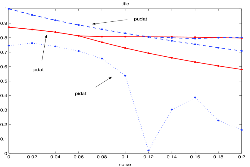
Figure 2: $p_{{\rm in}|{\rm out}}(i|i),\ i=1,2$ optimized for each noise level via (38) and (78).

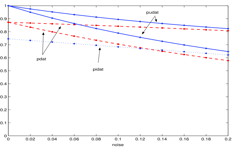
Figure 3: $p_{{\rm in}|{\rm out}}(i|i),\ i=1,2$ optimized only for the zero noise level.

6 Extensions and Other Considerations

6.1 Uncertain dynamics

The goal is to design the POVM $\{O_{i}\}$ in the presence of uncertain detector dynamics $Q\in{\mathbf{D}}_{\rm dyn}$ as illustrated in Figure 4.

$$\rho\in{\mathbf{D}}_{\rm in}\Longrightarrow\framebox{$\displaystyle\begin{array}[]{c}\mbox{Uncertain Dynamics}\\ Q\in{\mathbf{D}}_{\rm dyn}\end{array}$}\Longrightarrow\framebox{$\displaystyle\begin{array}[]{c}\mbox{POVM}\\ \{O_{i}\}\end{array}$}\Longrightarrow d\in{\mathbf{D}}_{\rm out}$$

Figure 4: Detector with uncertain dynamics.

We will assume that ${\mathbf{D}}_{\rm dyn}$ consists of a finite number of unitary operators $\{U_{k}\}$ with corresponding occurrence probabilities $\{p_{\rm dyn}(k)\}$. Thus,

$$\begin{array}[]{rcl}{\mathbf{D}}_{\rm dyn}&=&\left\{\,U_{k}\in{\bf C}^{n\times n}\,\left|\,k=1,\ldots,\ell\,\right.\right\}\\ p_{\rm dyn}(k)&=&{\bf Prob}\left\{Q=U_{k}\right\}\end{array}$$ (96)

The conditional probability (18) now becomes,

$$p_{{\rm out}|{\rm in}}(i|j)={\bf Tr}\ O_{i}\hat{\rho}_{j}\ ,\;\;\;\;\hat{\rho}_{j}=\sum_{k=1}^{\ell}\ p_{\rm dyn}(k)U_{k}\rho_{j}U_{k}^{*}$$ (97)

This clearly shows that the only changes to make is to replace $\rho_{j}$ with $\hat{\rho}_{j}$ everywhere, specifically, in the error probabilities (22) and in the output state $\rho$ as defined by (20).

The above representation of $Q$ is an example of a the more generic Kraus operator sum representation (OSR). Specifically, the Kraus matrices, $\left\{\,K_{k}\in{\bf C}^{n\times n}\,\left|\,k=1,\ldots,\ell\,\right.\right\}$ with $\ell\leq n^{2}$, can characterize a large class of possibilities for the $Q$-system as follows:

$$Q(\rho,K)=\sum_{k=1}^{\ell}\ K_{k}\rho K_{k}^{*},\;\;\;\sum_{k=1}^{\ell}\ K_{k}^{*}K_{k}=K_{0}\leq I_{n}$$ (98)

Comparing this with (96) gives $K_{k}=\sqrt{p_{\rm dyn}(k)}U_{k}$ and $K_{0}=I_{n}$, which clearly is just one possibility. For example, when $K_{0}<I_{n}$, additional measurement operations within $Q$ are included. The OSR also accounts for many forms of error sources as well as decoherence, e.g., [34], [31].

6.2 Detector with fixed POVM

In this section we consider designing the detector for a fixed POVM set. We will show that the detector dynamics when represented as an OSR (Operator-Sum-Representation) can also be designed by solving a quasiconvex optimization problem.

Suppose we are given the POVM, $\{O_{i}\}$, and wish to design $Q$ for optimal detection as shown in Figure 5.

$$\rho\in{\mathbf{D}}_{\rm in}\Longrightarrow\framebox{$\displaystyle\begin{array}[]{c}\mbox{Detector}\\ Q\end{array}$}\Longrightarrow\framebox{$\displaystyle\begin{array}[]{c}\mbox{Fixed POVM}\\ \{O_{i}\}\end{array}$}\Longrightarrow d\in{\mathbf{D}}_{\rm out}$$

Figure 5: Detector with fixed POVM.

The POVM would be most likely selected as rank-one projectors in the natural basis. For example, for $i=1,\ldots,m$, fix $b_{i}\in{\mathbf{C}}^{m}$ and $O_{i}=I_{\ell}\otimes b_{i}\ b_{i}^{*}$ with $\ell+m=n$, the dimension of the input state. The input state might also consist of prepared ancilla states. In the natural basis $b_{1}^{T}=[1\ 0\ \cdots\ 0],\ b_{2}=[0\ 1\ 0\ \cdots\ 0],\ldots,b_{m}^{T}=[0\ \cdots\ 0\ 1]$.

As noted in Section 6.1, a very general form to characterize $Q$ is the Krause OSR. Using (98), the a posteriori performance probability is now,

$$p_{\rm post}(i)=\frac{p_{i}\ {\bf Tr}\ O_{i}\ Q(\rho_{i},K)}{{\bf Tr}\ O_{i}Q(\rho,K)}$$ (99)

which is quadratic (fractional) in the Kraus matrices. It can be transformed into a quasiconvex function by expanding the Kraus matrices in a fixed basis. The procedure, described in [34, §8.4.2], is as follows: since any matrix in ${\bf C}^{n\times n}$ can be represented by $n^{2}$ complex numbers, let

$$\left\{\,B_{\mu}\in{\bf C}^{n\times n}\,\left|\,\mu=1,\ldots,n^{2}\,\right.\right\}$$ (100)

be a basis for matrices in ${\bf C}^{n\times n}$. The Kraus matrices can thus be expressed as,

$$K_{k}=\sum_{\mu=1}^{n^{2}}\ a_{k\mu}B_{\mu},\;k=1,\ldots,\ell$$ (101)

where the $n^{2}$ coefficients $\{a_{k\mu}\}$ are complex scalars. As shown in [34] the representation (98) now becomes,

$$Q(\rho,X)=\sum_{\mu,\nu=1}^{n^{2}}\ X_{\mu\nu}\ B_{\mu}\rho B_{\nu}^{*},\;\;\;\sum_{\mu,\nu=1}^{n^{2}}\ X_{\mu\nu}\ B_{\mu}^{*}B_{\nu}\leq I_{n}$$ (102)

with

$$X_{\mu\nu}=\sum_{k=1}^{\ell}\ a_{k\mu}^{*}a_{k\nu},\;\;\;\mu,\nu=1,\ldots,n^{2}$$ (103)

The matrix $X\in{\mathbf{C}}^{n^{2}\times n^{2}}$ with the above coefficients must also be non-negative in order to maintain probabilities. The number of free (real) variables in $X$ is thus $n^{4}-n^{2}$. In addition, we can write,

$$p_{\rm out}(i)={\bf Tr}\ O_{i}\ Q(\rho,X)={\bf Tr}\ XR_{i}(\rho),\;i=1,\ldots,m$$ (104)

where the matrix $R_{i}(\rho)\in{\mathbf{C}}^{n^{2}\times n^{2}}$ has elements given by,

$$[R_{i}(\rho)]_{\mu\nu}={\bf Tr}\ B_{\nu}\rho B_{\mu}^{*}O_{i},\;\mu,\nu=1,\ldots,n^{2}$$ (105)

The problem of optimally designing the “system” part of the detector, the $Q$-system, is equivalent to the following optimization problem over the positive semidefinite matrix $X\in{\mathbf{C}}^{n^{2}\times n^{2}}$.

$$\begin{array}[]{ll}\mbox{minimize}&\left\|e_{\rm post}\right\|_{\rm wc}=\displaystyle\max_{i=1,\ldots,m}\ w_{i}\ \left(1-\frac{p_{i}\ {\bf Tr}\ XR_{i}(\rho_{i})}{{\bf Tr}\ XR_{i}(\rho)}\right)\\ \mbox{subject to}&\sum_{\mu\nu}\ X_{\mu\nu}\ B_{\mu}^{*}B_{\nu}\leq I_{n},\;\;\;X\geq 0\end{array}$$ (106)

This problem, like (38), is also a quasiconvex optimization problem with the optimization variables being the elements of the matrix $X$.

Implementation of OSR

An OSR can be implemented using unitary operations (and if necessary projection measurements) and the $X$-matrix can be transformed to Kraus operators via the singular value decomposition [34]. Specifically, let $X=VSV^{*}$ with unitary $V\in{\mathbf{C}}^{n^{2}\times n^{2}}$ and $S={\rm diag}(s_{1}\ \cdots\ s_{n^{2}})$ with the singular values ordered so that $s_{1}\geq s_{2}\geq\ \cdots\ \geq s_{n^{2}}\geq 0$. Then the coefficients in the basis representation of the Kraus matrices (101) are,

$$a_{k\mu}=\sqrt{s_{k}}\ V_{\mu k}^{*},\ k,\mu=1,\ldots,n^{2}$$ (107)

Theoretically there can be fewer then $n^{2}$ Kraus operators. For example, if the $Q$ system is unitary, then,

$$Q(\rho)=U\rho U^{*}$$ (108)

In effect, there is one Kraus operator, $U$, which is unitary and of the same dimension as the input state $\rho$. The corresponding $X$ matrix is a dyad, hence ${\bf rank}\ X=1$. Adding a rank constraint would thus force a simplification of the implementation. Unfortunately, a rank constraint is not convex. However, the $X$ matrix is symmetric and positive semidefinite, hence the heuristic from [19] applies where the rank constraint is replaced by the trace constraint,

$${\bf Tr}\ X\leq\eta$$ (109)

From the singular value decomposition of $X$, ${\bf Tr}\ X=\sum_{k}s_{k}$. Adding the constraint (109) to (106) will force some (or many) of the $s_{k}$ to be small which can be eliminated (post-optimization) thereby reducing the rank. The auxiliary parameter $\eta$ can be used to find a tradeoff between simpler realizations and performance.

Appendix A Optimality Conditions

Optimality conditions are derived from Lagrange Duality Theory for the following detection criteria: (i) average joint performance, (ii) worst-case a posteriori performance with noise-free measurements, and (iii) worst-case a posteriori performance with noisy measurements.

Caveat emptor The material in this section is meant to be a “scaffold” to what can be found in some of the recent texts on convex optimization, e.g., see [5] and the references therein. More specifically, we refer principally to the sections in [5] where detailed information and proofs can be found for any axiomatic statements made here. The same caution applies to our references to computational methods: interested readers should refer directly to the available convex solvers which can be downloaded from the web, e.g., sdpsol [43] or sedumi [42].

A.1 Optimality conditions for average joint performance

We will apply Lagrange Duality Theory [5, Ch.5] to the optimization problem (23) referred to in this context as the primal problem. The Lagrange function associated with the primal problem (23) is,

$$L(O,Z,Y)=\sum_{i=1}^{m}\ {\bf Tr}\ O_{i}A_{i}-{\bf Tr}\ Z_{i}O_{i}+{\bf Tr}\ Y\Big{(}I_{n}-\sum_{i=1}^{m}\ O_{i}\Big{)}$$ (110)

with Lagrange multipliers $Z_{i}\in{\bf C}^{n\times n},\ Z_{i}\geq 0$ for the inequality constraint $O_{i}\geq 0$, and $Y\in{\mathbf{R}}^{n\times n},\ Y=Y^{T}$ for the equality constraint $\sum_{i=1}^{m}\ O_{i}=I_{n}$. The first term in $L(O,Z,Y)$ is the objective function in (23) expressed in terms of the data matrices $A_{i}$ from (25). The Lagrange dual function is defined as,,

$$\begin{array}[]{rcl}g(Z,Y)&=&\displaystyle\inf_{O}\ L(O,Z,Y)\\ &=&\left\{\begin{array}[]{ll}{\bf Tr}\ Y&A_{i}-Z_{i}-Y=0,\ i=1,\ldots,m\\ -\infty&\mbox{otherwise}\end{array}\right.\end{array}$$ (111)

One of the important properties of the dual function is that for any $Z_{i}\geq 0$ and any $Y$, we get the lower bound,

$$g(Z,Y)\leq\delta^{\rm opt}$$ (112)

where $\delta^{\rm opt}$ is the optimal objective value from solving (23). The Lagrange dual problem establishes the largest lower bound from,

$$\begin{array}[]{ll}\mbox{maximize}&g(Z,Y)\\ \mbox{subject to}&Z_{i}\geq 0,\;i=1,\ldots,m\end{array}$$ (113)

where the optimization variables are $(Z,Y)$. Using (111) we can eliminate the $Z_{i}$ variables and write the dual problem explicitly in terms of the $Y$ variables as,

$$\begin{array}[]{ll}\mbox{maximize}&{\bf Tr}\ Y\\ \mbox{subject to}&A_{i}-Y\geq 0,\;i=1,\ldots,m\end{array}$$ (114)

A solution, $Y^{\rm opt}$, the dual optimal multiplier, also returns the maximum objective value, $d^{\rm opt}={\bf Tr}\ Y^{\rm opt}$, the dual optimal value. From (112) we get $d^{\rm opt}\leq\delta^{\rm opt}$. A numerical solution of the primal problem (23) always returns $\hat{\delta}\geq\delta^{\rm opt}$, and likewise numerically solving the dual problem (114) will always return $\hat{d}\leq d^{\rm opt}$. Thus, the optimal solution is always contained in the known interval $\hat{d}\leq d^{\rm opt}\leq s^{\rm opt}\leq\hat{s}$ . For this primal-dual pair we also have strong duality, that is, $d^{\rm opt}=s^{\rm opt}$. This follows because the primal problem satisfies Slater’s condition [5, §5.2.3], which in this case means that the primal problem is convex and there exist strictly feasible $(O_{i})$, i.e., $O_{i}>0,\;i=1,\ldots,m,\;\sum_{i=1}^{m}\ O_{i}=I_{n}$. (For example, let $O_{i}=I_{n}/m$). The optimal and computed objective values then satisfy,

$$\hat{d}\leq{\bf Tr}\ Y^{\rm opt}=\delta^{\rm opt}\leq\hat{\delta}$$ (115)

Strong duality also implies the following complementary slackness conditions, [5, §5.5.2],

$$\begin{array}[]{rcl}Z^{\rm opt}_{i}O^{\rm opt}_{i}=\left(A_{i}-Y^{\rm opt}\right)O^{\rm opt}_{i}&=&0,\;i=1,\ldots,m\end{array}$$ (116)

The last line uses $Z_{i}=A_{i}-Y$ from (111). Combining $\sum_{i=1}^{m}\ O^{\rm opt}_{i}=I$ with $(A_{i}-Y^{\rm opt})O^{\rm opt}_{i}=0,\;i=1,\ldots,m$ gives,

$$Y^{\rm opt}=\sum_{i=1}^{m}\ A_{i}O^{\rm opt}_{i}$$ (117)

This can be used in to eliminate $Y^{\rm opt}$ in (114) and (116) yielding the constraints,

$$\begin{array}[]{rcl}A_{i}-\sum_{j=1}^{m}\ A_{j}O_{j}&\geq&0,\;i=1,\ldots,m\\ \left(A_{i}-\sum_{j=1}^{m}\ A_{j}O_{j}\right)O_{i}&=&0,\;i=1,\ldots,m\end{array}$$ (118)

These are the conditions stated in (24) as being necessary and sufficient for optimality of any feasible POVM set $\{O_{i}\}$. The proof of this statement relies on the fact that if strong duality holds and the primal problem is convex – both true for this problem – then the above conditions (118) are equivalent to the Karush-Kuhn-Tucker (KKT) conditions for optimality, which in this case are both necessary and sufficient [5, §5.5.3]. Thus, any feasible POVM set which satisfies (118) is optimal.

A.2 Optimality conditions for worst-case a posteriori performance

As shown in [5, §4.2.5], a solution to the quasiconvex optimization problem (38) can be obtained by solving a series of convex feasibility problems together with a bisection method. We start with the equivalence,

$$\left\|e_{\rm post}\right\|_{\rm wc}\leq\delta\Leftrightarrow w_{i}\left(1-\frac{p_{i}\ {\bf Tr}\ O_{i}\ \rho_{i}}{{\bf Tr}\ O_{i}\rho}\right)\leq\delta\Leftrightarrow\left\{\begin{array}[]{l}{\bf Tr}\ O_{i}A_{i}(\delta)\leq 0\\ \\ A_{i}(\delta)=(w_{i}-\delta)\rho-w_{i}p_{i}\rho_{i}\end{array}\right.$$ (119)

Problem (38) is then equivalent to,

$$\begin{array}[]{ll}\mbox{minimize}&\delta\\ \mbox{subject to}&{\bf Tr}\ O_{i}A_{i}(\delta)\leq 0\\ &\sum_{i=1}^{m}\ O_{i}=I_{n},\;\;\;O_{i}\geq 0,\;i=1,\ldots,m\end{array}$$ (120)

where the variables are now the real scalar $\delta$ as well as the POVM matrices $\{O_{i}\in{\bf C}^{n\times n}\}$. The algorithm below requires knowing an upper and lower bound on the optimal $\delta^{\rm opt}$. Without loss of generality we can normalize the weights so that $0\leq w_{i}\leq 1$. Since the objective is a weighted error probability, the feasible range is $0\leq\delta^{\rm opt}\leq 1$. The bisection algorithm as presented in [5, §4.2.5] now becomes:

Bisection-Feasibility Method

given $\delta_{\min}=0,\ \delta_{\max}=1$, tolerance $\epsilon>0$.

repeat

1. $\delta=(\delta_{\min}+\delta_{\max})/2$

2. Solve the convex feasibility problem

   $$\begin{array}[]{ll}\mbox{find}&O_{i},\;i=1,\ldots,m\\ \mbox{subject to}&{\bf Tr}\ O_{i}A_{i}(\delta)\leq 0\\ &\sum_{i=1}^{m}\ O_{i}=I_{n},\;\;\;O_{i}\geq 0,\;i=1,\ldots,m\end{array}$$ (121)

3. if feasible, $\delta_{\max}=\delta$; else $\delta_{\min}=\delta$

until $\delta_{\max}-\delta_{\min}\leq\epsilon$.

The feasibility step is equivalent to solving the following SDP in the variables $(s,O_{i})$:

$$\begin{array}[]{ll}\mbox{minimize}&s\\ \mbox{subject to}&{\bf Tr}\ O_{i}A_{i}(\delta)\leq s\\ &\sum_{i=1}^{m}\ O_{i}=I_{n},\;\;\;O_{i}\geq 0,\;i=1,\ldots,m\end{array}$$ (122)

Let $s^{\rm opt},\ O^{\rm opt}_{i}$ denote the optimal solution. Under the temporary assumption that ${\bf Tr}\ O_{i}^{\rm opt}\rho>0$, the inequality ${\bf Tr}\ O_{i}^{\rm opt}A_{i}(\delta)\leq s^{\rm opt}$ is equivalent to,

$$\left\|e_{\rm post}\right\|_{\rm wc}=\max_{i}\ w_{i}\left(1-\frac{p_{i}{\bf Tr}\ O_{i}^{\rm opt}\rho_{i}}{{\bf Tr}\ O_{i}^{\rm opt}\rho}\right)\leq\delta+\frac{s^{\rm opt}}{\min_{i}\ {\bf Tr}\ O_{i}^{\rm opt}\rho}$$ (123)

It follows that if $s^{\rm opt}>0$ then $\delta$ is feasible, and hence, $\delta^{\rm opt}<\delta$. If $s^{\rm opt}<0$ then $\delta$ is infeasible, i.e., $\delta^{\rm opt}>\delta$. The optimal value $\delta^{\rm opt}$ is clearly the solution to $s^{\rm opt}(\delta^{\rm opt})=0$. The bisection algorithm together with using an interior-point method to solve the SDP (122) will return a value of $\delta$ to within any desired, but finite, accuracy of the optimal.

The key computational step is solving the feasibility problem (122). High quality code which uses an interior-point method is recommended such as those found in sdpsol [43] or sedumi [42]. In many cases the optimal POVM matrices are rank deficient which may result in a large condition number in the linear equations to be solved in the Newton step. This should not be a problem for well conceived code.

To obtain the optimality conditions we will now apply Lagrange Duality Theory to the feasibility problem (122) in the Bisection-Feasibility method. Problem (122) is the primal problem. As previously noted, the primal optimal value, $s^{\rm opt}(\delta)$, determines if $\delta$ is feasible, Specifically,

$$\begin{array}[]{rcl}s^{\rm opt}<0&\Leftrightarrow&\delta>\delta^{\rm opt}\\ s^{\rm opt}>0&\Leftrightarrow&\delta<\delta^{\rm opt}\\ s^{\rm opt}=0&\Leftrightarrow&\delta=\delta^{\rm opt}\end{array}$$ (124)

The Lagrange function associated with the primal problem (122) is,

$$L(s,O,\lambda,Z,Y)=s+\sum_{i=1}^{m}\ \Big{(}\lambda_{i}({\bf Tr}\ O_{i}A_{i}(\delta)-s)-{\bf Tr}\ Z_{i}O_{i}\Big{)}+{\bf Tr}\ Y\Big{(}I_{n}-\sum_{i=1}^{m}\ O_{i}\Big{)}$$ (125)

with Lagrange multipliers $\lambda_{i}\in{\mathbf{R}},\ \lambda_{i}\geq 0$ for the inequality constraint ${\bf Tr}\ O_{i}A_{i}(\delta)\leq s$, $Z_{i}\in{\bf C}^{n\times n},\ Z_{i}\geq 0$ for the inequality constraint $O_{i}\geq 0$, and $Y\in{\mathbf{R}}^{n\times n},\ Y=Y^{T}$ for the equality constraint $\sum_{i=1}^{m}\ O_{i}=I_{n}$. The Lagrange dual function is then,

$$\begin{array}[]{rcl}g(\lambda,Z,Y)&=&\displaystyle\inf_{s,O}\ L(s,O,\lambda,Z,Y)\\ &=&\left\{\begin{array}[]{ll}{\bf Tr}\ Y&\sum_{i=1}^{m}\ \lambda_{i}=1,\;\lambda_{i}A_{i}(\delta)-Z_{i}-Y=0,\ i=1,\ldots,m\\ -\infty&\mbox{otherwise}\end{array}\right.\end{array}$$ (126)

The Lagrange dual problem establishes the largest lower bound from,

$$\begin{array}[]{ll}\mbox{maximize}&g(\lambda,Z,Y)\\ \mbox{subject to}&\lambda_{i}\geq 0,\;Z_{i}\geq 0,\;i=1,\ldots,m\end{array}$$ (127)

where the optimization variables are $(\lambda,Z,Y)$. Using (126) we can eliminate the $Z_{i}$ variables and write the dual problem explicitly in terms of the $\lambda_{i}$ and $Y$ variables as,

$$\begin{array}[]{ll}\mbox{maximize}&{\bf Tr}\ Y\\ \mbox{subject to}&\lambda_{i}\geq 0,\;\lambda_{i}A_{i}(\delta)-Y\geq 0,\;i=1,\ldots,m\\ &\sum_{i=1}^{m}\ \lambda_{i}=1\end{array}$$ (128)

The dual optimal solution is $(\lambda^{\rm opt},\ Y^{\rm opt})$. Strong duality also holds for this problem because Slater’s condition holds [5, §5.2.3]: there exist strictly feasible $(s,\ O_{i})$, such that ${\bf Tr}\ O_{i}A_{i}(\delta)<s,\;O_{i}>0,\;i=1,\ldots,m,\;\sum_{i=1}^{m}\ O_{i}=I_{n}$. Since the primal (feasibility) problem is convex, the optimal primal and dual objective values are equal,

$${\bf Tr}\ Y^{\rm opt}=s^{\rm opt}$$ (129)

Strong duality also implies the following complementary slackness conditions, [5, §5.5.2],

$$\begin{array}[]{rcl}\lambda^{\rm opt}_{i}\ \left({\bf Tr}\ O^{\rm opt}_{i}A_{i}(\delta)-s^{\rm opt}\right)&=&0,\;i=1,\ldots,m\\ Z^{\rm opt}_{i}O^{\rm opt}_{i}=\left(\lambda_{i}^{\rm opt}A_{i}(\delta)-Y^{\rm opt}\right)O^{\rm opt}_{i}&=&0,\;i=1,\ldots,m\end{array}$$ (130)

The last line uses $Z_{i}=\lambda_{i}A_{i}(\delta)-Y$ from (126). Combining $\sum_{i=1}^{m}\ O^{\rm opt}_{i}=I$ with $(\lambda^{\rm opt}_{i}A_{i}(\delta^{\rm opt})-Y^{\rm opt})O^{\rm opt}_{i}=0,\;i=1,\ldots,m$ gives,

$$Y^{\rm opt}=\sum_{i=1}^{m}\ \lambda^{\rm opt}_{i}A_{i}(\delta)O^{\rm opt}_{i}$$ (131)

We now put all the primal and dual equality and inequality constraints together at the optimal $\delta=\delta^{\rm opt}$, $s^{\rm opt}={\bf Tr}\ Y^{\rm opt}=0$, and use (131) to eliminate $Y^{\rm opt}$. To simplify notation we drop the superscript $(\cdot)^{\rm opt}$ from all the variables $(O,\lambda,Y,Z,\delta)$. This gives:

$$\begin{array}[]{rcl}\sum_{i=1}^{m}\ O_{i}&=&I\\ O_{i}&\geq&0,\;i=1,\ldots,m\\ \lambda_{i}{\bf Tr}\ O_{i}A_{i}(\delta)&=&0,\;i=1,\ldots,m\\ \lambda_{i}A_{i}(\delta)-\sum_{j=1}^{m}\ \lambda_{j}A_{j}(\delta)O_{j}&\geq&0,\;i=1,\ldots,m\\ \left(\lambda_{i}A_{i}(\delta)-\sum_{j=1}^{m}\ \lambda_{j}A_{j}(\delta)O_{j}\right)O_{i}&=&0,\;i=1,\ldots,m\\ \lambda_{i}&\geq&0,\;i=1,\ldots,m\\ \sum_{i=1}^{m}\ \lambda_{i}&=&1\end{array}$$ (132)

These can also be established directly from the KKT conditions for optimality which in this case are both necessary and sufficient [5, §5.5.3]. For the linear constraints, either the constraint is active, ${\bf Tr}\ A_{i}(\delta)O_{i}=0,\ \lambda_{i}>0$, or inactive, ${\bf Tr}\ A_{i}(\delta)O_{i}<0,\ \lambda_{i}=0$. Combining this with (132) gives the optimality conditions in (43).

Suppose the weights are all equal with $w_{i}=1,\ \forall i$. Then,

$$A_{i}(\delta)=\gamma\rho-p_{i}\rho_{i}\equiv A_{i}(\gamma)$$ (133)

with $\gamma=1-\delta$. From now on we will use $A_{i}(\gamma)$ or $A_{i}(\delta)$ as appropriate to the context.

Suppose the optimal is achieved by only one constraint, that is, for $i=k$, ${\bf Tr}\ O_{k}A_{k}(\gamma)=0$ and for $i\neq k$, ${\bf Tr}\ O_{i}A_{i}(\gamma)<0$. Then, $\lambda_{k}=1$, $\lambda_{i\neq k}=0$ and the optimality conditions (132) reduce to,

$$\begin{array}[]{rcl}A_{k}(\gamma)\left(I-O_{k}\right)&\geq&0\\ A_{k}(\gamma)O_{k}&\leq&0\\ A_{k}(\gamma)\left(I-O_{k}\right)O_{k}&=&0\\ A_{k}(\gamma)O_{k}O_{i}&=&0,\;i\neq k\\ {\bf Tr}\ O_{k}A_{k}(\gamma)&=&0\end{array}$$ (134)

Since $\rho>0$ by assumption (21),

$$\begin{array}[]{rcl}\det\ A_{k}(\gamma)&=&\det\ \left(\rho^{1/2}\left(\gamma I-p_{k}\rho^{-1/2}\rho_{k}\rho^{-1/2}\right)\rho^{1/2}\right)\\ &=&(\det\ \rho)\ \prod_{j=1}^{n}\ \left(\gamma-p_{k}\omega_{kj}\right)\end{array}$$

with $\omega_{kj},\ j=1,\ldots,n$ the eigenvalues of $\rho^{-1/2}\rho_{k}\rho^{-1/2}$. Because $\rho>0,\ \rho_{k}\geq 0$, they are all non-negative and $\max_{j}\omega_{kj}>0$. Let $\gamma=p_{k}\max_{j}\omega_{kj}$, or equivalently,

$$\gamma=p_{k}\ \sigma_{\max}(\rho^{-1/2}\rho_{k}\rho^{-1/2})$$ (135)

where $\sigma_{\max}(\cdot)$ is the maximum singular value of the matrix argument. With this choice $\det A_{k}(\gamma)=0$ and hence $A_{k}(\gamma)=0$ has the decomposition:

$$\begin{array}[]{l}A_{k}(\gamma)=\left[U_{k+}\ U_{k0}\right]\ \left[\begin{array}[]{cc}\Omega_{k+}&0_{n-1}\\ 0_{n-1}^{T}&0\end{array}\right]\ \left[\begin{array}[]{c}U_{k+}^{*}\\ U_{k0}^{*}\end{array}\right]\\ \\ \Omega_{k+}={\bf diag}(\omega_{1},\ldots,\omega_{n-1}),\;\omega_{1}\geq\omega_{2}\geq\cdots\geq\omega_{n-1}\geq 0,\;\;\omega_{1}>0\end{array}$$ (136)

for unitary $[U_{k+}\ U_{k0}]$ with $U_{k+}\in{\mathbf{C}}^{n\times n-1}$ and $U_{k0}\in{\mathbf{C}}^{n\times 1}$. Setting,

$$O_{k}=U_{k0}U_{k0}^{*},\;\;I-O_{k}=U_{k+}U_{k+}^{*}$$ (137)

gives $A_{k}(\gamma)O_{k}=U_{k+}\Omega_{k+}U_{k+}^{*}\geq 0,\ A_{k}(\gamma)(I-O_{k})=0,\ O_{k}(I-O_{k})=0$, thus satisfying the optimality conditions. Observe also that $O_{k}$ is a rank $1$ projector, and $I-O_{k}$ is a rank $n-1$ projector. Also, $I-O_{k}=\sum_{i\neq k}O_{i}$, and hence is the sum of the remaining $m-1$ POVM elements. These are thus arbitrary except for satisfying (137) with each $O_{i}\geq 0,\ i\neq k$.

Since the single active constraint $k$ can occur for any $i=1,\ldots,m$, then,

$$\gamma=\min_{i=1,\ldots,m}\ p_{i}\sigma_{\max}(\rho^{-1/2}\rho_{i}\rho^{-1/2})$$ (138)

which establishes (47) as the optimal objective value for equal weights with one active linear constraint. More specifically, this means that there is a single index $k\in{1\ldots,m}$ such that $\gamma=p_{k}\sigma_{\max}(\rho^{-1/2}\rho_{k}\rho^{-1/2})<p_{i}\sigma_{\max}(\rho^{-1/2}\rho_{i}\rho^{-1/2}),\;\forall i\neq k$.

The same procedure involving the decomposition (136) is used to arrive at the results for single pure state detection with weights $w_{1}=1,\ w_{2}=0$ given by (54)-(56).

A.3 Optimality conditions for worst-case a posteriori performance with noisy measurements

To apply the Bisection-Feasibility Method as described in the previous section, replace $O_{i}$ with $O_{i}^{\rm noisy}$ everywhere in (122). Thus the primal (feasibility) problem becomes,

$$\begin{array}[]{ll}\mbox{minimize}&s\\ \mbox{subject to}&{\bf Tr}\ O_{i}^{\rm noisy}A_{i}(\delta)\leq s\\ &O_{i}^{\rm noisy}=\sum_{j=1}^{m}\ \nu_{ij}O_{j},\;i=1,\ldots,m\\ &\sum_{i=1}^{m}\ O_{i}=I_{n},\;\;\;O_{i}\geq 0,\;i=1,\ldots,m\end{array}$$ (139)

The Lagrange function is then,

$$L(s,O,\lambda,Z,Y)=s+\sum_{j=1}^{m}\ \lambda_{j}({\bf Tr}\ O_{j}^{\rm noisy}A_{j}(\delta)-s)-\sum_{i=1}^{m}\ {\bf Tr}\ Z_{i}O_{i}+{\bf Tr}\ Y\Big{(}I_{n}-\sum_{i=1}^{m}\ O_{i}\Big{)}$$ (140)

with Lagrange multipliers $\lambda_{i}\in{\mathbf{R}},\ \lambda_{i}\geq 0$ for the inequality constraint ${\bf Tr}\ O_{i}^{\rm noisy}A_{i}(\delta)\leq s$, $Z_{i}\in{\bf C}^{n\times n},\ Z_{i}\geq 0$ for the inequality constraint $O_{i}\geq 0$, and $Y\in{\mathbf{R}}^{n\times n},\ Y=Y^{T}$ for the equality constraint $\sum_{i=1}^{m}\ O_{i}=I_{n}$. Eliminating the noisy POVM terms gives,

$$L(s,O,\lambda,Z,Y)={\bf Tr}\ Y+s\left(1-\sum_{i=1}^{m}\lambda_{i}\right)+\sum_{i=1}^{m}\ {\bf Tr}\ O_{i}\left(A_{i}(\delta,\nu)-Z_{i}-Y\right)$$ (141)

with the $A_{i}(\delta,\nu)$ given by (65). Although not shown, the optimality conditions (64) can be established by repeating, mutadis mutandis, all the steps in the previous section, i.e., formulate the dual problem, show that strong duality holds, and so on.

References

- [1] K. Audenaert and B. De Moor. Optimizing completely positive maps using semidefinite programming. Phys. Rev. A, 65, 2003.
- [2] M. Ban, K. Kurokawa, R. Momose, and O. Hirota. Optimum measurements for discrimination among symmetric quantum states and parameter estimation. Int. J. Theor. Phys., 36:1269–1288, 1997.
- [3] K. Banaszek. Optimal receiver for quantum cryptography with two coherent states. Phys. Lett. A, 253:12–15, 1999.
- [4] S. M. Barnett and E. Riis. J. Mod. Opt., 44(1061), 1997.
- [5] S. Boyd and L. Vandenberghe. Convex Optimization. Cambridge University Press, 2004. also available at www.stanford.edu/boyd/cvxbook.html.
- [6] M. Charbit, C. Bendjaballah, and C. W. Helstrom. Cutoff rate for the -ary PSK modulation channel with optimal quantum detection. IEEE Trans. Inform. Theory, 35:1131–1133, Sep. 1989.
- [7] A. Chefles. Unambiguous discrimination between linearly independent quantum states. Phys. Lett. A, 239:339–347, Apr. 1998.
- [8] A. Chefles. Quantum state discrimination. Contemporary Physics, 41:401–424, 2000.
- [9] A. Chefles and S. M. Barnett. Optimum unambiguous discrimination between linearly independent symmetric states. Phys. Lett. A, 250:223–229, 1998.
- [10] R. B. Clarke, V. Kendon, A. Chefles, S. M. Barnett, E. Riis, and M. Saski. Phys. Rev. A, XXX, 2001.
- [11] D. Dieks. Overlap and distinguishability of quantum states. Phys. Lett. A, 126:303–307, 1988.
- [12] Y. C. Eldar. Mixed quantum state detection with inconclusive results. Phys. Rev. A, 67:042309–1:042309–14, Apr. 2003.
- [13] Y. C. Eldar. A semidefinite programming approach to optimal unambiguous discrimination of quantum states. IEEE Trans. Inform Theory, 49:446–456, Feb. 2003.
- [14] Y. C. Eldar. von neumann measurement is optimal for detecting linearly independent mixed quantum states. Phys. Rev. A, 68:052303–1:052303–4, 2003.
- [15] Y. C. Eldar and G. D. Forney, Jr. On quantum detection and the square-root measurement. IEEE Trans. Inform. Theory, 47:858–872, Mar. 2001.
- [16] Y. C. Eldar, A. Megretski, and G. C. Verghese. Optimal detection of symmetric mixed quantum states. quant-ph/0211111, 2002.
- [17] Y. C. Eldar, A. Megretski, and G. C. Verghese. Designing optimal quantum detectors via semidefinite programming. IEEE Trans. Inform. Theory, 49:1012–1017, Apr. 2003.
- [18] Y. C. Eldar, M. Stojnic, and B. Hassibi. Optimal quantum detectors for unambiguous detection of mixed states. Phys. Rev. A, 2003. to appear.
- [19] M. Fazel, H. Hindi, and S. P. Boyd. A rank minimization heuristic with application to minimum order system approximation. Proc. American Control Conference, 6:4734–4739, June 2001.
- [20] J. Fiurášek and M. Ježek. Optimal discrimination of mixed quantum states involving inconclusive results. Phys. Rev. A, 67:012321, 2003.
- [21] L. Gonick and W. Smith. The Cartoon Guide to Statistics. Harper-Collins, 1993.
- [22] W. Grice and I. A. Walmsley. J. Mod. Opt, 1995.
- [23] C. W. Helstrom. Quantum Detection and Estimation Theory. New York: Academic Press, 1976.
- [24] C. W. Helstrom. Bayes-cost reduction algorithm in quantum hypothesis testing. IEEE Trans. Inform. Theory, 28:359–366, Mar. 1982.
- [25] A. S. Holevo. Statistical decisions in quantum theory. J. Multivar. Anal., 3:337–394, Dec. 1973.
- [26] B. Huttner, A. Muller, J. D. Gautier, H. Zbinden, and N. Gisin. Unambiguous quantum measurement of nonorthogonal states. Phys. Rev. A, 54:3783–3789, 1996.
- [27] I. D. Ivanovic. How to differentiate between non-orthogonal states. Phys. Lett. A, 123:257–259, Aug. 1987.
- [28] G. Jaeger and A. Shimony. Optimal distinction between two non-orthogonal quantum states. Phys. Lett. A, 197:83–87, 1995.
- [29] E. Knill, R. Laflamme, and G. Milburn. A scheme for efficient quantum computation using linear optics. Nature, 409(46), 2001.
- [30] R. L. Kosut, I. A. Walmsley, and H. Rabitz. Optimal experiment design for quantum state and process tomography. 2004. in preparation; preprint avialble by email request to kosut@scsolutions.com.
- [31] D. A. Lidar, Z. Bihary, and K.B. Whaley. From completely positive maps to the quantum markovian semigroup master equation. Chemical Physics, 268(35), 2001.
- [32] S. Lloyd and L. Viola. Control of open quantum system dynamics. arXiv:quant-ph/0008101 24, Aug. 2000.
- [33] K. Nemoto and S. Braunstein. Phys. Rev. A, 2000.
- [34] M. A. Nielsen and I. L. Chuang. Quantum Computation and Quantum Information. Cambridge, 2000.
- [35] M. Osaki, M. Ban, and O. Hirota. Derivation and physical interpretation of the optimum detection operators for coherent-state signals. Phys. Rev. A, 54:1691–1701, Aug. 1996.
- [36] A. Peres. How to differentiate between non-orthogonal states. Phys. Lett. A, 128:19, Mar. 1988.
- [37] A. Peres. Quantum Theory: Concepts and Methods. Boston: Kluwer, 1995.
- [38] A. Peres and D. R. Terno. Optimal distinction between non-orthogonal quantum states. J. Phys. A, 31:7105–7111, 1998.
- [39] S. J. D. Phoenix, S. M. Barnett, and A. Chefles. J. Mod. Opt., 47(507), 2000.
- [40] R. Raussendorf and H. J. Briegel. A one-way quantum computer. Phys. Rev. Lett., 86(5188), 2001.
- [41] T. Rudolph, R. W. Spekkens, and P. S. Turner. Unambiguous discrimination of mixed states. Phys. Rev. A, 68:010301–1–010301–4, 2003.
- [42] J. F. Sturm. Using sedumi 1.02, a matlab toolbox for optimization over symmetric cones. Optimization Methods and Software, 11-12:625–653, 1999. Special issue on Interior Point Methods; available from fewcal.kub.nl/sturm/software/sedumi.html.
- [43] S.-P. Wu and S. Boyd. Sdpsol: a parser/solver for sdp and maxdet problems with matrix structure. 2000. Chapter in Advances in Linear Matrix Inequality Methods in Control, edited by L. El Ghaoui and S.-I. Niculescu, SIAM.
- [44] H. P. Yuen, R. S. Kennedy, and M. Lax. Optimum testing of multiple hypotheses in quantum detection theory. IEEE Trans. Inform. Theory, IT-21:125–134, Mar. 1975.
- [45] C. W. Zhang, C. F. Li, and G. C. Guo. General strategies for discrimination of quantum states. Phys. Lett. A, 261:25–29, 1999.