Phase diagram for the Grover algorithm with static imperfections

Abstract

We study effects of static inter-qubit interactions on the stability of the Grover quantum search algorithm. Our numerical and analytical results show existence of regular and chaotic phases depending on the imperfection strength $\varepsilon$. The critical border $\varepsilon_{c}$ between two phases drops polynomially with the number of qubits $n_{q}$ as $\varepsilon_{c}\sim n_{q}^{-3/2}$. In the regular phase $(\varepsilon<\varepsilon_{c})$ the algorithm remains robust against imperfections showing the efficiency gain $\varepsilon_{c}/\varepsilon$ for $\varepsilon\gtrsim 2^{-n_{q}/2}$. In the chaotic phase $(\varepsilon>\varepsilon_{c})$ the algorithm is completely destroyed.

Quantum computations open new perspectives and possibilities for treatment of complex computational problems in a more efficient way with respect to algorithms based on the classical logic Nielsen . In the quantum computers classical bits are replaced by two-level quantum systems (qubits) and classical operations with bits are substituted by elementary unitary transformations (quantum gates). The elementary gates can be reduced to single qubit rotations and controlled two-qubit operations, e.g. control-NOT gate Nielsen . Combinations of elementary gates allow to implement any unitary operation on a quantum register, which for $n_{q}$ qubits contains exponentially many states $N=2^{n_{q}}$. The two most famous quantum algorithms are the Shor algorithm for integer number factorization Shor94 and the Grover quantum search algorithm Grov97 . The Shor algorithm is exponentially faster than any known classical algorithm, while the Grover algorithm gives a quadratic speedup.

In realistic quantum computations the elementary gates are never perfect and therefore it is very important to analyze the effects of imperfections and quantum errors on the algorithm accuracy. A usual model of quantum errors assumes that angles of unitary rotations fluctuates randomly in time for any qubit in some small interval $\varepsilon$ near the exact angle values determined by the ideal algorithm. In this case a realistic quantum computation remains close to the ideal one up to a number of performed gates $N_{g}\sim 1/\varepsilon^{2}$. For example, the fidelity $f$ of computation, defined as a square of scalar product of quantum wavefunctions of ideal and perturbed algorithms, remains close to unity if a number of performed gates is smaller than $N_{g}$. This result has been established analytically and numerically in extensive studies of various quantum algorithms Cirac95 ; Paz ; Geor01 ; Song02 ; Terra03 ; Bett03 ; Frahm03 .

Another source of quantum errors comes from internal imperfections generated by residual static couplings between qubits and one-qubit energy level shifts which fluctuate from one qubit to another but remain static in time. These static imperfections may lead to appearance of many-body quantum chaos, which modifies strongly the hardware properties of realistic quantum computer Geor00 ; Berman ; BeneEPJD . The effects of static imperfections on the accuracy of quantum computation have been investigated on the examples of quantum algorithms for the models of complex quantum dynamics Bene01 ; Pome04 ; Terra03 ; Frahm03 . As a result a universal law for fidelity decay induced by static imperfections has been established Frahm03 for quantum algorithms simulating dynamics in the regime of quantum chaos. At the same time it has been realized that the effects of static imperfections for dynamics in an integrable regime are not universal and more complicated. Therefore it is important to investigate the effects of static imperfections on an example of the well known Grover algorithm. First attempt was done recently in Braun02 , but the global picture of the phenomenon remained unclear. In this paper we present extensive numerical and analytical studies which establish the global stability diagram of reliable operability of the Grover algorithm.

Let us first outline the key features of the Grover algorithm Grov97 . An unstructured database is presented by $N=2^{n_{q}}$ states of quantum register with $n_{q}$ qubits: $\{|x\rangle\}$, $x=0,\ldots,N-1$. The searched state $|\tau\rangle$ can be identified by oracle function $g(x)$, defined as $g(x)=1$ if $x=\tau$ and $g(x)=0$ otherwise. The Grover iteration operator $\hat{G}$ is a product of two operators: $\hat{G}=\hat{D}\hat{O}$. Here the oracle operator $\hat{O}=(-1)^{g(\hat{x})}$ is specific to the searched state $|\tau\rangle$, while the diffusion operator $\hat{D}$ is independent of $|\tau\rangle$: $D_{ii}=-1+\frac{2}{N}$ and $D_{ij}=\frac{2}{N}\;\;(i\neq j)$. For the initial state $|\psi_{0}\rangle=\sum_{x=0}^{N-1}|x\rangle/\sqrt{N}$, $t$ applications of the Grover operator $\hat{G}$ give Nielsen :

$$|\psi(t)\rangle=\hat{G}^{t}|\psi_{0}\rangle=\sin{((t+1)\omega_{G})}|\tau\rangle+\cos{((t+1)\omega_{G})}|\eta\rangle\;,$$ (1)

where the Grover frequency $\omega_{G}=2\arcsin(\sqrt{1/N})$ and $|\eta\rangle=\sum_{x\neq\tau}^{(0\leq x<N)}|x\rangle/\sqrt{N-1}$. Hence, the ideal algorithm gives a rotation in the 2D plane $(|\tau\rangle,|\eta\rangle)$.

The implementation of the operator $D$ through the elementary gates requires an ancilla qubit. As a result the Hilbert space becomes a sum of two subspaces $\{|x\rangle\}$ and $\{|x+N\rangle\}$, which differ only by a value of $(n_{q}+1)$-th qubit. These subspaces are invariant with respect to operators $O$ and $D$: $O=1-2|\tau\rangle\langle\tau|-2|\tau+N\rangle\langle\tau+N|$, $D=1-2|\psi_{0}\rangle\langle\psi_{0}|-2|\psi_{1}\rangle\langle\psi_{1}|$, where $|\psi_{1}\rangle=\sum_{x=0}^{N-1}|x+N\rangle/\sqrt{N}$ and $|\psi_{0,1}\rangle$ correspond to up/down ancilla states. Then $D$ can be represented as $D=WRW$ Grov97 , where the transformation $W=W_{n_{q}}\ldots W_{k}\ldots W_{1}$ is composed from $n_{q}$ one-qubit Hadamard gates $W_{k}$, and $R$ is the $n_{q}$-controlled phase shift defined as $R_{ij}=0$ if $i\neq j$, $R_{00}=1$ and $R_{ii}=-1$ if $i\neq 0$ $(i,j=0,\ldots,N-1)$. In turn, this operator can be represented as $R=W_{n_{q}}\sigma^{x}_{n_{q}-1}\ldots\sigma^{x}_{1}\wedge_{n_{q}}\sigma^{x}_{n_{q}-1}\ldots\sigma^{x}_{1}W_{n_{q}}$, where $\wedge_{n_{q}}$ is generalized $n_{q}$-qubit Toffolli gate, which inverts the $n_{q}$-th qubit if the first $n_{q}-1$ qubits are in the state $|1\rangle$. The construction of $\wedge_{n_{q}}$ from $3$-qubit Toffolli gates with the help of only one auxillary qubit is described in Bare95 . As a result the Grover operator G is implemented through $n_{g}=12n_{tot}-42$ elementary gates including one-qubit rotations, control-NOT and Toffolli gates. Here $n_{tot}=n_{q}+1$ is the total number of qubits.

To study effects of static imperfections on the Grover algorithm we use the model introduced in Geor00 . In this model a quantum computer hardware is described by the Hamiltonian $H$:

$$H=\sum_{i}\frac{\Delta}{2}\sigma_{i}^{z}+H_{S},\;\;H_{S}=\sum_{i}a_{i}\sigma_{i}^{z}+\sum_{i<j}b_{ij}\sigma^{x}_{i}\sigma^{x}_{j}.$$ (2)

Here, $\sigma_{i}$ are the Pauli matrices for qubits $i$, and $\Delta$ is an average one-qubit energy spacing. All $n_{tot}$ qubits are placed on a rectangular lattice, the second sum in $H_{S}$ runs over nearest neighbor qubits with periodic boundary conditions. Qubit energy shifts $a_{i}$ and couplings $b_{ij}$ are randomly and uniformly distributed in the intervals $\left[-\alpha,\alpha\right]$ and $\left[-\beta,\beta\right]$, respectively. Following Bene01 ; Terra03 ; Frahm03 ; Pome04 we assume that the average spacing $\Delta$ is compensated by specially applied laser pulses so that between subsequent elementary gates the wavefunction evolution is given by the propagator $U_{S}=\exp(-iH_{S}t_{g})$. Thus all static errors are expressed via this propagator while the elementary gates are taken to be perfect. Appropriate rescaling of parameters $a_{i}$ and $b_{ij}$ allows to put $t_{g}=1$ without any loss of generality. We concentrate our studies on the case $\alpha=\beta\equiv\varepsilon$ where inter-qubit couplings lead to a developed quantum chaos Geor00 ; Bene01 .

Figure 1: Probability of searched state $w_{G}(t)$ (top) and fidelity $f(t)$ (bottom) as a function of the iteration step $t$ in the Grover algorithm for $n_{tot}=12$ qubits. Dotted curves show results for the ideal algorithm $(\varepsilon=0)$, dashed and solid curves correspond to imperfection strength $\varepsilon=4\cdot 10^{-4}$ and $10^{-3}$, respectively.

A typical example of imperfection effects on the accuracy of the Grover algorithm is shown in Fig.1 for a fixed disorder realization of $H_{S}$ in (2) on $3\times 4$ qubit lattice. It clearly shows that imperfections suppress the probability $w_{G}$ to find the searched state, where $w_{G}$ is given by a sum of probabilities of states $|\tau\rangle$ and $|\tau+N\rangle$. In contrast to the case of time-dependent random quantum errors studied in Song02 in the case of static imperfections the oscillations of probability $w_{G}$ do not decrease with time $t$. Another interesting feature is a significant decrease of the period of the Grover oscillations compared to the case of ideal algorithm, where $T_{G}=\pi/2\omega_{G}$. This effect is also absent in the case of random errors. The fidelity of quantum computation $f(t)$ also shows non-decaying oscillations at large times. However, in average the maxima of fidelity correspond to minima rather than maxima of probability $w_{G}$. Hence, $f(t)$ is not appropriate for tests of the algorithm accuracy.

Following Hus-Paz a pictorial presentation of the dynamical evolution in the Grover algorithm can be obtained with the help of the Husimi function Husimi , which is shown in Fig.2. In this presentation the computational basis $x$ can be considered as a coordinate space representation for the wavefunction $\psi_{x}(t)$ ($x=0,\ldots,2N-1$), while the conjugated basis obtained by the Fourier transform corresponds to momentum representation $p$ ($p=-N+1,\ldots,N$). In this way the initial state of the Grover algorithm $|\psi_{0}\rangle$ gives a peaked distribution with $p=0$. In the ideal algorithm the total probability is distributed between two states $|\tau\rangle$ and $|\eta\rangle$ (see Eq.(1)) that gives two orthogonal lines in the phase space of Husimi function (see Fig.2, top raw). After the period $T_{G}\approx 34$ all the probability is transferred to the target state $|\tau\rangle$ ($w_{G}\approx 1$). In the presence of moderate imperfections the flips of the ancilla qubit become possible that involves into dynamics two additional states. As a result the probability is mainly distributed over four states corresponding to four straight lines in phase space (Fig.2, middle raw):

$$\begin{array}[]{ll}|\tau_{0}\rangle=|\tau\rangle&|\tau_{1}\rangle=|\tau+N\rangle\\ |\eta_{0}\rangle=|\eta\rangle&|\eta_{1}\rangle=\sum_{x\neq\tau}^{(0\leq x<N)}|x+N\rangle/\sqrt{N-1}\end{array}.$$ (3)

The probability $w_{4}$ contained in these states is close to unity (in Fig.2 $w_{4}=0.998$ for $\varepsilon=10^{-3}$). Above certain critical border $\varepsilon_{c}$ this simple structure is completely washed out ($w_{4}=6\cdot 10^{-4}$), and the Husimi function shows only random distribution (Fig.2, bottom raw).

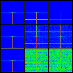
Figure 2: (Color) Evolution of the Husimi function in the Grover algorithm at times $t=0$, 17, and $34$ (from left to right), and for $\varepsilon=0$, 0.001, and 0.008 (from top to bottom). The qubit lattice and disorder realization are the same as in Fig.1. The vertical axis shows the computational basis $x=0,\ldots,2N-1$, while the horizontal axis represents the conjugated momentum basis. Density is proportional to color changing from maximum (red) to zero (blue).

The dominant contribution of these four states can be also seen in spectral density $S(\omega)$ of the wavefunction $\psi_{x}(t)$. This density is defined as: $S(\omega)=\sum_{x}|a_{x}(\omega)|^{2}$, where $a_{x}(\omega)=\sum_{t=0}^{T_{f}}\psi_{x}(t)\exp(i\omega t)/\sqrt{T_{f}}$ and $T_{f}$ is a large time scale on which the spectrum is determined (we usually used $T_{f}\approx 5T_{G}\gg T_{G}$). The phase diagram of spectral density $S(\omega)$ dependence on the imperfection strength $\varepsilon$ is shown in Fig.3. Two phases are clearly seen: for $\varepsilon<\varepsilon_{c}$ the diagram contains four lines corresponding to the four states (3), while for $\varepsilon>\varepsilon_{c}$ these lines are destroyed and the spectrum becomes continuous. These phases correspond to the qualitative change of the Husimi distribution shown in Fig.2.

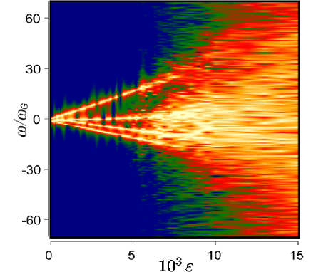
Figure 3: (Color) Phase diagram for the spectral density $S(\omega)$ as a function of imperfection strength $\varepsilon$, $n_{tot}=12$, same disorder realization as in Fig.2. Color is proportional to density $S(\omega)$ (yellow for maximum and blue for zero).

To study the transition between these phases in a more quantitative way we analyze the dependence of probabilities $w_{G}$ and $w_{4}$ on the imperfection strength $\varepsilon$ for a large number of disorder realizations in $H_{S}$ (2) changing also the number of qubits $n_{tot}$. The number of realizations vary from 50 to 1000 depending on $\varepsilon$ and $n_{tot}$. Since the frequency of Grover oscillations varies strongly with $\varepsilon$ and disorder we average $w_{G}$ and $w_{4}$ over a large time interval $T_{f}$ to suppress fluctuations in time. The obtained results are summarized in Fig.4. For a fixed value of $n_{tot}$ the dependence $w_{G}(\varepsilon)$ changes strongly from one realization to another (Fig.4a). In contrast, the probability $w_{4}$ remains close to unity being insensitive to variations of disorder up to $\varepsilon<\varepsilon_{c}$ (Fig.4b). Only for $\varepsilon>\varepsilon_{c}$, when $w_{4}\ll 1$, it becomes sensitive to disorder. The probabilities averaged over disorder $\bar{w}_{G}$ and $\bar{w}_{4}$ are shown in Fig.4a,b. They also have a qualitative change in behavior near $\varepsilon_{c}$, especially $\bar{w}_{4}$. These results confirm the fact that the phase transition takes place near some critical $\varepsilon_{c}$ for an ensemble of disorder realizations.

The value of $\varepsilon_{c}$ can be obtained from the following estimate. The transition rate induced by imperfections after one Grover iteration is given by the Fermi golden rule: $\Gamma\sim\varepsilon^{2}n_{g}^{2}n_{tot}$, where $n_{tot}$ appears due to random contribution of qubit couplings $\varepsilon$ while $n_{g}^{2}$ factor takes into account coherent accumulation of perturbation on $n_{g}$ gates used in one iteration (see, e.g. Frahm03 ). In the Grover algorithm the four states (3) are separated from all other states by energy gap $\Delta E\sim 1$ (it appears due to sign change introduced by operators $O$ and $D$). Thus these four states become mixed with all others for

$$\varepsilon>\varepsilon_{c}\approx 1.7/(n_{g}\sqrt{n_{tot}})$$ (4)

when $\Gamma>\Delta E$. Here the numerical factor is obtained from numerical data. The parameter dependence is well confirmed by data for $\bar{w}_{4}$ shown in Fig.4d.

The variation of averaged Grover probability $\bar{w}_{G}$ with $\varepsilon$ and $n_{tot}$ is presented in Fig.4c. The dependence on system parameters can be understood on the basis of simple single-kick model. In this model the action of static imperfections in all gates entering in one Grover iteration is replaced by a single kick unitary operator $U_{eff}=\exp{(-iH_{s}n_{g}R)}$ acting after each iteration. Here $R$ is a dimensionless renormalization factor which takes into account that gates do not commute with $H_{S}$. Figs.4a,b show that this single kick approximation gives a good description of original averaged data with $R=0.56$. Thus, the renormalization effects play a significant role and therefore this model does not describe the probability variation for a given disorder realization. However, the averaged dependence is correctly reproduced.

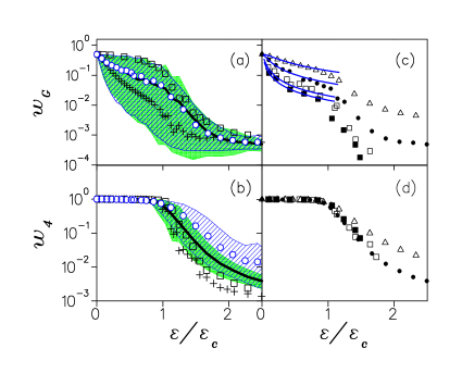
Figure 4: (Color online) Dependence of probabilities $w_{G}$ (a,c) and $w_{4}$ (b,d) on rescaled imperfection strength $\varepsilon/\varepsilon_{c}$, with $\varepsilon_{c}$ from (4). For panels (a,b) $n_{tot}=12$, squares and pluses show data for two typical disorder realizations, green/grey area shows the region of probability variation for various disorder realizations (see text), full thick curves give average dependence $\bar{w}_{G}$, $\bar{w}_{4}$. Dashed area bounded by thin curves show the region of probability variation in the single-kick model, open circles give the average data in this model with rescaling factor $R=0.56$. Panels (c,d) show $\bar{w}_{G}$, $\bar{w}_{4}$ for $n_{tot}=9$ (triangles), 12 (full circles), 15 (open squares) and 16 (full squares). In panel (c) full curves are given by Eq.(6) for same $n_{tot}$ values from top to bottom, $R=0.56$.

In the regime where the dynamics of Grover algorithm is dominated by four states subspace (3) the single-kick model can be treated analytically. The matrix elements of the effective Hamiltonian in this space are

$$H_{eff}=\left(\begin{array}[]{cccc}A+a&0&-i\omega_{G}&0\\ 0&A-a&0&-i\omega_{G}\\ i\omega_{G}&0&B&b\\ 0&i\omega_{G}&b&B\\ \end{array}\right),$$ (5)

where $A=-Rn_{g}\sum_{i=1}^{n_{q}}a_{i}\langle\tau|\sigma_{i}^{(z)}|\tau\rangle$, $B=Rn_{g}\sum_{i<j}^{n_{q}}b_{i,j}-b$, $a=-Rn_{g}a_{n_{q}+1}$ and $b=Rn_{g}(b_{n_{q}+1,n_{q}+2-L_{x}}+b_{n_{q}+1,L_{x}}+b_{n_{q},n_{q}+1}+b_{n_{q}+1-L_{x},n_{q}+1})$ and qubits are arranged on $L_{x}\times L_{y}$ lattice, and numerated as $i=x+L_{x}(y-1)$, with $x=1,\ldots,L_{x}$, $y=1,\ldots,L_{y}$. In the limit of large $n_{q}$ the terms $a,b$ are small compared to $A,B$ by a factor $1/\sqrt{n_{q}}$ and $H_{eff}$ is reduced to $2\times 2$ matrix, which gives $w_{G}=2\omega_{G}^{2}/[(A-B)^{2}+4\omega_{G}^{2}]$. For large $n_{q}$ the difference $A-B$ has a Gaussian distribution with width $\sigma=Rn_{g}\sqrt{n_{q}/3}\sqrt{\alpha^{2}+2\beta^{2}}=\varepsilon Rn_{g}\sqrt{n_{q}}$. The convolution of $w_{G}$ with this distribution gives

$$\bar{w}_{G}=\sqrt{\pi/2}(1-\operatorname{erf}(\sqrt{2}\omega_{G}/\sigma))\exp{(2\omega_{G}^{2}/\sigma^{2})}\;\omega_{G}/\sigma$$ (6)

This formula gives a good description of numerical data in Fig.4c that confirms the validity of single-kick model. For $\sigma\gg\omega_{G}$ and a typical disorder realization with $(A-B)\sim\sigma$ the actual frequency of Grover oscillations is strongly renormalized: $\omega\approx(A-B)\sim\sigma\gg\omega_{G}$, and in agreement with Fig.3 $\omega\sim\varepsilon/\varepsilon_{c}$. In this typical case $w_{G}\sim\omega_{G}^{2}/\sigma^{2}\ll 1$ (almost total probability is in the states $|\eta_{0}\rangle$,$|\eta_{1}\rangle$). Hence, the total number of quantum operations $N_{op}$, required for detection of searched state $|\tau\rangle$, can be estimated as $N_{op}\sim N_{M}/\omega\sim\sigma/\omega_{G}^{2}\sim\varepsilon N/\varepsilon_{c}$, where $N_{M}\sim 1/w_{G}\sim\sigma^{2}/\omega_{G}^{2}$ is a number of measurements required for detection of searched state note . Thus, in presence of strong static imperfections the parametric efficiency gain of the Grover algorithm compared to classical one is of the order $\varepsilon_{c}/\varepsilon$. For $\varepsilon\sim\omega_{G}$ the efficiency is comparable with that of the ideal Grover algorithm while for $\varepsilon\sim\varepsilon_{c}$ there is no gain compared to the classical case.

In summary, we have shown that the Grover algorithm remains robust against static imperfections inside a well defined domain and determined the dependence of algorithm efficiency on the imperfection strength.

This work was supported in part by the EU IST-FET project EDIQIP and the NSA and ARDA under ARO contract No. DAAD19-01-1-0553.

References

- (1) M.A. Nielsen, I.L. Chuang, Quantum Computation and Quantum Information, Cambridge Univ. Press, Cambridge (2000).
- (2) P.W. Shor, in Proceedings of th 35th Annual Simposium on Foundation of Computer Science, Ed. S. Goldwasser (IEEE Computer Society, Los Alamos, CA, 1994), p. 124.
- (3) L.K. Grover, Phys. Rev. Lett. 79, 325 (1997).
- (4) J.I. Cirac and P. Zoller, Phys. Rev. Lett. 74, 4091 (1995).
- (5) C. Miguel, J.P. Paz and W.H. Zurek, Phys. Rev. Lett. 78, 3971 (1997).
- (6) B. Georgeot and D.L. Shepelyansky, Phys. Rev. Lett. 86, 5393 (2001)
- (7) P.H. Song and I. Kim, Eur. Phys. J. D 23, 299 (2003).
- (8) M. Terraneo and D.L. Shepelyansky, Phys. Rev. Lett. 90, 257902 (2003).
- (9) S. Bettelli, quant-ph/0310152.
- (10) K.M. Frahm and D.L. Shepelyansky, quant-ph/0312120.
- (11) B.Georgeot and D.L.Shepelyansky, Phys. Rev. E 62, 3504 (2000); 62, 6366 (2000).
- (12) G.P. Berman, F. Borgonovi, F.M. Izrailev, and V.I. Tsifrinovich, Phys. Rev. E 64, 056226 (2001).
- (13) G. Benenti, G. Casati, and D.L. Shepelaynsky, Eur. Phys. J. D 17, 265 (2001).
- (14) G. Benenti, G. Casati, S. Montangero, and D.L. Shepelaynsky, Phys. Rev. Lett. 87, 227901 (2001).
- (15) A.A. Pomeransky, D.L. Shepelaynsky, Phys. Rev. A 69, 014302 (2004).
- (16) D. Braun, Phys. Rev. A 65, 042317 (2002).
- (17) A. Barenco,et al., Phys. Rev. A 52, 3457 (1995).
- (18) C. Miquel, J.P. Paz and M. Saraceno, Phys. Rev. A 65, 062309 (2002).
- (19) S.-J. Chang and K.-J. Shi, Phys. Rev. A 34, 7 (1986).
- (20) Here we consider only the subspace (3), a small probability leakage to all other states is not crucial since it will be randomly distributed over states.