Entanglement at the boundary of spin chains near a quantum critical point and in systems with boundary critical points

Abstract

We analyze the entanglement properties of spins (qubits) attached to the boundary of spin chains near quantum critical points, or to dissipative environments, near a boundary critical point, such as Kondo-like systems or the dissipative two level system. In the first case, we show that the properties of the entanglement are significantly different from those for bulk spins. The influence of the proximity to a transition is less marked at the boundary. In the second case, our results indicate that the entanglement changes abruptly at the point where coherent quantum oscillations cease to exist. The phase transition modifies significantly less the entanglement.

I Introduction

Quantum phase transitions have attracted intense research activities on various fields of physicsSachdev (1999). Whereas classical phase transitions are driven by thermal fluctuations, quantum transitions are induced by a parameter which enhances quantum fluctuations at zero temperature. For simple models there is a correspondence between classical and quantum phase transitions such that the universal behavior of a $D$-dimensional quantum field theory corresponds to the critical behavior of a $D+1$-dimensional classical field theory. There are phenomena, however, which cannot easily be understood in terms of this correspondence, like the nature of the entanglement of the ground state wavefunction (see also Belitz et al. (2004)). The entanglement properties of the quantum wavefunction of a device are crucial for determining its suitability as part of a quantum computer (see, for instance Galindo and Martin-Delgado (2002)).

Recently, Osterloh et. al.Osterloh et al. (2002) discussed entanglement for the translationally invariant transversal Ising model in one dimension (see alsoOsborne and Nielsen (2002)). The authors observed that the derivative of the concurrence with respect to the coupling constant scales according to the Ising universality class close to the quantum phase transition. The concurrence is a measure of entanglement between only two spin-$1/2$ systemsWootters (1998), but also suitable to characterize entanglement also between next-nearest neighbors.Osborne and Nielsen (2002) The entanglement in the transverse Ising and XY models made up of macroscopic (contiguous) subsystems has been discussed inVidal et al. (2003), employing the von Neuman entropy as measure of entanglement. The analysis of the entanglement properties near a quantum critical point can be relevant to the analysis of many quantum algorithms, as the Hamiltonians used to implement them show gapless behavior at some point in the computationLatorre and Orus (2003); Orus and Latorre (2003).

We analyze here the entanglement properties of two level systems which are either attached to bulk systems tuned near a quantum phase transition, or which undergo a boundary phase transition, as described, for instance, by the dissipative two level systemLeggett et al. (1987); Weiss (1999), or the Kondo modelHewson (1997). These localized phase transitions are due to the coupling to a gapless (critical) environmentbqc . We will not consider, on the other hand, the entanglement between qubits as function of their separationVerstraete et al. (2004a, b), even though we distinguish between next and nearest-next neighbors.

We consider in the next section the properties of qubits at the boundary of the Ising model in a transverse field, i.e., the model studied inOsterloh et al. (2002); Osborne and Nielsen (2002). We analyze how the entanglement between the two last qubits varies as function of the distance to the quantum critical point of the model. We also allow the values of the couplings at the boundary to vary. In section III we discuss the entanglement properties of two spins attached to a critical reservoir, as the coupling between them varies, inducing a boundary critical point. We give the main conclusions of our work in section IV.

II The Ising model

We start from the homogeneous Ising model with open boundary conditions characterized by the parameter $\lambda$. The two spins at the end are further connected by an additional coupling parameter $\kappa$. The Hamiltonian is thus given by

$${\cal H}=-\lambda\sum_{i=1}^{N-1}\sigma_{i}^{x}\sigma_{i+1}^{x}-\sum_{i=1}^{N}\sigma_{i}^{z}-\kappa\sigma_{1}^{x}\sigma_{N}^{x}$$ (1)

where $\sigma_{i}^{x,z}$ are the $x,z$-components of the Pauli matrices.

To solve the model,Lieb et al. (1961); Pfeuty (1970) we first convert all the spin matrices to spinless fermions. This is done by performing the well-known Jordan-Wigner transformation ($\{c_{i},c_{i^{\prime}}^{\dagger}\}=\delta_{i,i^{\prime}}$):

$$\sigma_{i}^{x} =\exp\left(i\pi\sum_{j=1}^{i-1}c_{j}^{\dagger}c_{j}\right)(c_{i}+c_{i}^{\dagger})$$ (2)

$$\sigma_{i}^{z} =1-2c_{i}^{\dagger}c_{i}$$ (3)

As usual, we will neglect the term that involves the operator $\exp(i\pi{\cal N})$, ${\cal N}=\sum_{i=1}^{N}c_{i}^{\dagger}c_{i}$ in order to preserve the bilinearity of the model. An additional Bogoliubov transformation then yields (up to a constant)

$${\cal H}=\sum_{n=1}^{N}\omega_{n}\eta_{n}^{\dagger}\eta_{n}\quad,$$ (4)

$$\eta_{n}=\sum_{i=1}^{N}(g_{n,i}c_{i}+h_{n,i}c_{i}^{\dagger})$$ (5)

where the $g_{n,i}$, $h_{n,i}$, and $\omega_{n}$ are determined numerically (for the general case). Due to the unitarity of the Bogoliubov transformation, Eq. (5) is easily inverted to yield

$$c_{i}=\sum_{n=1}^{N}(g_{n,i}\eta_{n}+h_{n,i}\eta_{n}^{\dagger})\quad.$$ (6)

II.1 Concurrence

We are interested in the reduced density matrix $\rho(i,j)$ represented in the basis of the eigenstates of $\sigma_{z}$. It is formally obtained from the ground-state wave function after having integrated out all spins but the ones at position $i$ and $j$. As measure of entanglement, we use the concurrence between the two spins, ${\cal C}(\rho(i,j))$. It is defined as

$${\cal C}(\rho(i,j))=\text{max}\{0,\lambda_{1}-\lambda_{2}-\lambda_{3}-\lambda_{4}\}$$ (7)

where the $\lambda_{i}$ are the (positive) square roots of the eigenvalues of $R=\rho\tilde{\rho}$ in descending order. The spin flipped density matrix is defined as $\tilde{\rho}=\sigma_{y}\otimes\sigma_{y}\rho^{*}\sigma_{y}\otimes\sigma_{y}$, where the complex conjugate $\rho^{*}$ is again taken in the basis of eigenstates of $\sigma^{z}$. It will be instructive to also consider the “generalized concurrence”

$${\cal C}^{*}(\rho(i,j))=\lambda_{1}-\lambda_{2}-\lambda_{3}-\lambda_{4}\quad.$$ (8)

The reduced density matrix $\rho(i,j)\to\rho$ - from now on we drop the indices $i$ and $j$ - can be related to correlation functions. For this, we write the ground-state wave function as the superposition of the four states

$$|\psi_{0}\rangle=|\uparrow\uparrow\rangle|\phi_{\uparrow\uparrow}\rangle+|\uparrow\downarrow\rangle|\phi_{\uparrow\downarrow}\rangle+|\downarrow\uparrow\rangle|\phi_{\uparrow\downarrow}\rangle+|\downarrow\downarrow\rangle|\phi_{\downarrow\downarrow}\rangle,$$

where the first ket denotes the $z$-projection of the two spins at position $i$ and $j$. The matrix element $\rho_{\uparrow\uparrow,\downarrow\downarrow}=\langle\phi_{\uparrow\uparrow}|\phi_{\downarrow\downarrow}\rangle$, e.g., is thus given by $\rho_{\uparrow\uparrow,\downarrow\downarrow}=\langle\sigma_{i}^{+}\sigma_{j}^{+}\rangle$, where $\sigma_{i}^{\pm}=(\sigma_{i}^{x}\pm\sigma_{i}^{y})/2$.

Due to the invariance of the Hamiltonian under $\sigma_{i}^{x}=-\sigma_{i}^{x}$, at least eight components of the reduced density matrix are zero (for finite $N$). The diagonal entries read:

$$\rho_{1}\equiv\rho_{\uparrow\uparrow,\uparrow\uparrow} =(1+\langle\sigma_{i}^{z}\rangle+\langle\sigma_{j}^{z}\rangle+\langle\sigma_{i}^{z}\sigma_{j}^{z}\rangle)/4$$ (9)

$$\rho_{2}\equiv\rho_{\uparrow\downarrow,\uparrow\downarrow} =(1-\langle\sigma_{i}^{z}\rangle+\langle\sigma_{j}^{z}\rangle-\langle\sigma_{i}^{z}\sigma_{j}^{z}\rangle)/4$$ (10)

$$\rho_{3}\equiv\rho_{\downarrow\uparrow,\downarrow\uparrow} =(1+\langle\sigma_{i}^{z}\rangle-\langle\sigma_{j}^{z}\rangle-\langle\sigma_{i}^{z}\sigma_{j}^{z}\rangle)/4$$ (11)

$$\rho_{4}\equiv\rho_{\downarrow\downarrow,\downarrow\downarrow} =(1-\langle\sigma_{i}^{z}\rangle-\langle\sigma_{j}^{z}\rangle+\langle\sigma_{i}^{z}\sigma_{j}^{z}\rangle)/4$$ (12)

The non-zero off-diagonal entries are

$$\rho_{+}\equiv\rho_{\uparrow\uparrow,\downarrow\downarrow} =\langle\sigma_{i}^{+}\sigma_{j}^{+}\rangle$$ (13)

$$\rho_{-}\equiv\rho_{\uparrow\downarrow,\downarrow\uparrow} =\langle\sigma_{i}^{+}\sigma_{j}^{-}\rangle\quad.$$ (14)

The positive square roots of the eigenvalues of $R$ are then given by $|\sqrt{\rho_{1}\rho_{4}}\pm\rho_{+}|$ and $|\sqrt{\rho_{2}\rho_{3}}\pm\rho_{-}|$. Due to the semi-definiteness of the density matrix $\rho$, we can drop the absolute values, i.e., $\sqrt{\rho_{1}\rho_{4}}\pm\rho_{+}$ and $\sqrt{\rho_{2}\rho_{3}}\pm\rho_{-}$.

We now define $I_{1}\equiv\rho_{1}\rho_{4}-\rho_{2}\rho_{3}=4(\langle\sigma_{i}^{z}\sigma_{j}^{z}\rangle-\langle\sigma_{i}^{z}\rangle\langle\sigma_{j}^{z}\rangle)$ and $I_{2}\equiv\rho_{+}^{2}-\rho_{-}^{2}=-\langle\sigma_{i}^{x}\sigma_{j}^{x}\rangle\langle\sigma_{i}^{y}\sigma_{j}^{y}\rangle$. For a homogeneous model, we have $I_{1}\geq 0$ and $I_{2}\geq 0$.Pfeuty (1970) The largest eigenvalue of Eq. (7) is thus given by $\lambda_{1}=\sqrt{\rho_{1}\rho_{4}}+|\rho_{+}|$ and the concurrence reads

$${\cal C}^{*}(i,j) =2(|\rho_{+}|-\sqrt{\rho_{2}\rho_{3}})\quad.$$ (15)

We note that the above expression also holds for the generalized boundary conditions. For a homogeneous system, it can be further simplified to

$${\cal C}^{*}(i,j) =({\cal O}_{i,j}-1)/2$$ (16)

where we introduced the total order ${\cal O}_{i,j}\equiv\sum_{\alpha=x,y,z}|\langle\sigma_{i}^{\alpha}\sigma_{j}^{\alpha}\rangle|$.

II.2 Numerical Results

II.2.1 Open boundary conditions

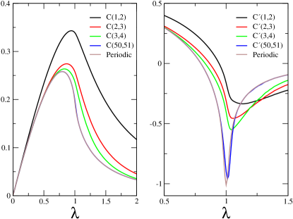
Figure 1: Left hand side: The nearest neighbor concurrence of the open boundary Ising model for different locations relative to the end as function of $\lambda$ for $N=101$. Right hand side: The derivative of the concurrence with respect to $\lambda$.

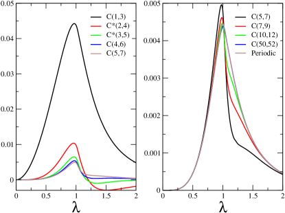
Figure 2: The next-nearest neighbor concurrence of the open boundary Ising model for different locations relative to the end of the chain as function of $\lambda$ for $N=101$.

We first consider the nearest neighbor concurrence of the Ising chain with open boundaries ($\kappa=0$) for a fixed number of sites $N=101$ as parameter of $\lambda$, but for various positions relative to the end of the chain. The results are displayed on the left hand side of Fig. 1. As expected, the concurrence of the periodic model is approached as one moves inside the chain and the difference between ${\cal C}(50,51)$ and ${\cal C}(i,i+1)$ of the periodic system is hardly seen. Nevertheless, the derivative of the concurrence with respect to the coupling parameter $\lambda$, ${\cal C}^{\prime}\equiv d{\cal C}/d\lambda$, still shows appreciable differences for $\lambda\approx 1$ (right hand side of Fig. 1).

We also investigated the scaling behavior of the minimum of ${\cal C}^{\prime}(1,2)$, $\lambda_{min}$, for different systems sizes up to $N=231$. We did not find finite-size scaling behavior for the position of the minimum as is the case for the translationally invariant modelOsterloh et al. (2002). The curve of ${\cal C}^{\prime}(1,2)$, shown on the right hand side of Fig. 1, is thus already close to the curve for $N\to\infty$ with a broad minimum around $\lambda_{min}\approx 1.1$.

The absence of finite-size scaling of the concurrence is also manifested in the case of the next-nearest neighbor concurrence for different system sizes $N$. Whereas for the periodic system the maximum of ${\cal C}(i,i+2)$ decreases monotonically for $N\to\infty$,Osterloh et al. (2002) there is practically no change of ${\cal C}(1,3)$ of the open chain for $N\lower 3.50006pt\hbox{$\stackrel{{\scriptstyle\textstyle>}}{{\sim}}$}51$.

In Fig. 2, the generalized next-nearest neighbor concurrence ${\cal C}^{*}(i,i+2)$ of the open boundary Ising model is shown for different locations relative to the end of the chain as function of $\lambda$ for $N=101$. On the left hand side of Fig. 2, results are shown for sites close to the end of the chain. Notice that the generalized concurrence becomes negative for $i=2,3$ for $\lambda>1$ which is not related to the quantum phase transition. The crossover of the boundary behavior to the bulk behavior is thus discontinuous. On the right hand side of Fig. 2, the next-nearest neighbor concurrence approaches the result of the system with periodic boundary conditions as one moves inside the chain.

II.2.2 Generalized boundary conditions

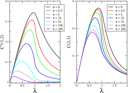
Figure 3: Left hand side: The (generalized) nearest neighbor concurrence of the closed Ising chain for various coupling strengths $\kappa$ as function of $\lambda$. Left hand side: ${\cal C}^{*}(1,2)$. Right hand side: ${\cal C}(2,3)$.

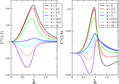
Figure 4: The generalized next-nearest neighbor concurrence of the closed Ising chain for various coupling strengths $\kappa$ as function of $\lambda$. Left hand side: ${\cal C}^{*}(1,3)$. Right hand side: ${\cal C}^{*}(2,4)$.

We now discuss the concurrence for the generalized boundary conditions, introducing the parameter $\kappa$. On the left hand side of Fig. 3, the generalized concurrence of the first two spins ${\cal C}^{*}(1,2)$ is shown as function of $\lambda$ for various coupling strengths $\kappa=0,..,20\lambda$ and $N=101$. For increasing $\kappa>0$, the curves indicate stronger non-analyticity at $\lambda\approx 1$. For $\kappa\lower 3.50006pt\hbox{$\stackrel{{\scriptstyle\textstyle>}}{{\sim}}$}20\lambda$, the generalized concurrence becomes negative around $\lambda=1$ and is ”significantly” positive only in the quantum limit of a strong transverse field ($\lambda<1$). A similar behavior of the concurrence is also found in the case of finite temperatures.Osborne and Nielsen (2002)

On the right hand side of Fig. 3, the concurrence of the second two spins ${\cal C}(2,3)$ is shown. All curves display similar behavior. There is thus a rapid crossover from the boundary to the bulk-regime and the concurrence of periodic boundary conditions is approached for all $\kappa$ as one moves further inside the chain.

To close, we discuss the next-nearest neighbor concurrence ${\cal C}(i,i+2)$ for various values of $\kappa$ and $N=101$. On the left hand side of Fig. 4, the generalized concurrence of the first and the third spin, ${\cal C}^{*}(1,3)$, is shown. For $\kappa\lower 3.50006pt\hbox{$\stackrel{{\scriptstyle\textstyle<}}{{\sim}}$}1$, ${\cal C}^{*}(1,3)$ is positive for all $\lambda$. For $\kappa\lower 3.50006pt\hbox{$\stackrel{{\scriptstyle\textstyle>}}{{\sim}}$}1$, ${\cal C}^{*}(1,3)$ first becomes negative for $\lambda<1$. For $\kappa\lower 3.50006pt\hbox{$\stackrel{{\scriptstyle\textstyle>}}{{\sim}}$}1.5$ ${\cal C}^{*}(1,3)$ is negative for all $\lambda$. On the right hand side of Fig. 4, the generalized concurrence of the second and the forth spin, ${\cal C}^{*}(2,4)$, is shown. For $\kappa\lower 3.50006pt\hbox{$\stackrel{{\scriptstyle\textstyle<}}{{\sim}}$}\lambda/2$, the ${\cal C}^{*}(2,4)$ is negative for $\lambda\lower 3.50006pt\hbox{$\stackrel{{\scriptstyle\textstyle>}}{{\sim}}$}1$. For $\kappa\lower 3.50006pt\hbox{$\stackrel{{\scriptstyle\textstyle>}}{{\sim}}$}3\lambda/2$, the ${\cal C}^{*}(2,4)$ is negative for $\lambda\lower 3.50006pt\hbox{$\stackrel{{\scriptstyle\textstyle<}}{{\sim}}$}1$. Nevertheless, the maximum value is close to $\lambda=1$ for all cases.

We finally note that the third neighbor concurrence remains zero for all $\lambda$ and all $\kappa$.

III Boundary Phase Transition

III.1 The model.

In order to observe critical behavior of the concurrence at the boundary, we thus have to consider a different model, i.e., we have to introduce an isotropic coupling from spin $N$ to spin $1$. This will introduce an interaction term which contains four fermionic operators and a simple solution is thus not possible anymore.

The model with isotropic coupling is similar to the model considered by Garst et. al., who discuss two Ising-coupled Kondo impuritiesGarst et al. (2003) (see alsoVojta et al. (2002)). We will consider the model studied inGarst et al. (2003). It describes to Kondo impurities, attached to two different electronic reservoirs, which interact among themselves through an Ising term. We can write the Hamiltonian as:

$${\cal H} = {\cal H}_{K1}+{\cal H}_{K2}+IS_{z1}S_{z2}$$

$${\cal H}_{Ki} = \sum_{k}\epsilon_{k,\mu}c^{{}^{\dagger}}_{k,\mu,i}c_{k,\mu,i}+J\sum_{k,k^{\prime},\mu,\nu}c_{k,\mu,i}\vec{\sigma}_{\mu,\nu}c_{k^{\prime},\nu,i}\vec{S}_{i}$$

We consider the entanglement of the two spins, by writing the $4\times 4$ reduced density matrix in terms of the values of $S_{z1}$ and $S_{z2}$.

The system described by Eq.(LABEL:hamil) undergoes a Kosterlitz-Thouless transition between a phase with a doubly degenerate ground state and a phase with a non degenerate ground state. This transition is equivalent to that in the dissipative two level systemLeggett et al. (1987); Weiss (1999) as function of the strength of the dissipation. We define the dissipative two level system as:

$${\cal H}_{TLS}=\Delta\sigma_{x}+\sum_{k}|k|b^{{}^{\dagger}}_{k}b_{k}+\lambda\sigma_{z}\sum_{k}\sqrt{k}(b^{{}^{\dagger}}_{k}+b_{k})$$ (18)

The strength of the dissipation can be characterized by a dimensionless parameter, $\alpha\propto\lambda^{2}$, and the model undergoes a transition for $\tilde{\Delta}=\delta/\omega_{c}\ll 1$, where $\omega_{c}$ is the cutoff, and $\alpha=1$. The Kondo model can be mapped onto this modelGuinea et al. (1985) by taking $\Delta\propto\tilde{J_{\perp}}$ and $1-\alpha\propto\tilde{J_{z}}$.

To understand the equivalence between these two models, it is best to to consider the limit $I/J\gg 1$ (the transition takes place fr all values of this ratio). Let us suppose that $I>0$ so that the Ising coupling is antiferromagnetic. The Hilbert space of the two impurities has four states. The combinations $|\uparrow\uparrow\rangle$ and $|\downarrow\downarrow\rangle$ are almost decoupled from the low energy states, and the transition can be analyzed by considering only the $|\uparrow\downarrow\rangle$ and $|\downarrow\uparrow\rangle$ combinations. Thus, we obtain an effective two state system. The transition is driven by the spin flip processes described by the Kondo terms. These processes involve two simultaneous spin flips in the two reservoirs. Hence, the operator which induces these spin flips leads to the correspondence $\tilde{\Delta}\leftrightarrow J_{\perp}^{2}/(I\omega_{c})$. The scaling dimension of this term, in the Renormalization Group sense, is reduced with respect to the ordinary Kondo Hamiltonian, as two electron-hole pairs must be created. This implies the equivalence $2-\alpha\leftrightarrow\tilde{J_{z}}$. Hence, the transition, which for the ordinary Kondo system takes place when changing the sign of $J_{z}$ now requires a finite value of $J_{z}$.

III.2 Calculation of the concurrence.

The $4\times 4$ reduced density matrix can be decomposed into a $2\times 2$ box involving the states $|\uparrow\downarrow\rangle$ and $|\downarrow\uparrow\rangle$, which contains the matrix elements which are affected by the transition, and the remaining elements involving $|\uparrow\uparrow\rangle$ and $|\downarrow\downarrow\rangle$ which are small, and are not modified significantly by the transition. Neglecting these couplings, we find that two of the four eigenvalues of the density matrix are zero. The other two are determined by the matrix:

$$\tilde{\rho}\equiv\left(\begin{array}[]{cc}\frac{1}{2}+\langle\sigma_{z}\rangle&\langle\sigma_{x}\rangle\\ \langle\sigma_{x}\rangle&\frac{1}{2}-\langle\sigma_{z}\rangle\end{array}\right)$$ (19)

where the operator $\tilde{\sigma}$ is defined using the standard notation of the dissipative two level system, Eq.(18). The entanglement can be written as:

$${\cal C}=\sqrt{\langle\sigma_{z}\rangle^{2}+\langle\sigma_{x}\rangle^{2}}$$ (20)

The value of $\langle\sigma_{z}\rangle$ is the order parameter of the transition. The value of $\langle\sigma_{x}\rangle$, at zero temperature, can be calculated from:

$$\langle\sigma_{x}\rangle=\frac{\partial E}{\partial\Delta}$$ (21)

where $E$ is the energy of the ground state. Using renormalization group arguments, it can be written as:

$$E=\left\{\begin{array}[]{lr}\frac{C}{1-2\alpha}\left[\Delta\left(\frac{\Delta}{\omega_{c}}\right)^{\frac{\alpha}{1-\alpha}}-\frac{\Delta^{2}}{\omega_{c}}\right]&0<\alpha<\frac{1}{2}\\ 2C\frac{\Delta^{2}}{\omega_{c}}\log\left(\frac{\omega_{c}}{\Delta}\right)&\alpha=\frac{1}{2}\\ \frac{C}{2\alpha-1}\left[\frac{\Delta^{2}}{\omega_{c}}-\Delta\left(\frac{\Delta}{\omega_{c}}\right)^{\frac{\alpha}{1-\alpha}}\right]&\frac{1}{2}<\alpha<1\\ C\left(\frac{\Delta^{2}}{\omega_{c}}-C^{\prime}\omega_{c}e^{-\frac{C^{\prime\prime}\omega_{c}}{\Delta}}\right)&\alpha\sim 1\\ C\frac{\Delta^{2}}{\omega_{c}}&\alpha>1\end{array}\right.$$ (22)

where $C,C^{\prime}$ and $C^{\prime\prime}$ are numerical constants.

If the density matrix is calculated in the absence of a symmetry breaking field, $\langle\sigma_{z}\rangle=0$ even in the ordered phase. Then, from Eq.(20), the concurrence is given by ${\cal C}=|\langle\sigma_{x}\rangle|$, which is completely determined using Eqs.(21) and (22). In the limit $\Delta/\omega_{c}\ll 1$ the interaction with the environment strongly suppresses the entanglement. We expect unusual behavior of the concurrence for $\alpha=1/2$ and $\alpha=1$. The point $\alpha=1/2$ marks the loss of coherent oscillations between the two statesGuinea (1985); not , although the ground state remains non degenerate. Following the analysis inOsterloh et al. (2002), we analyze the behavior of $\partial{\cal C}/\partial\alpha$, as $\alpha$ is the parameter which determines the position of the critical point. The strongest divergence of this quantity occurs for $\alpha=1/2$, where:

$$\left.\frac{\partial{\cal C}}{\partial\alpha}\right|_{\alpha=1/2}\sim\frac{\Delta}{\omega_{c}}\log\left(\frac{\omega_{c}}{\Delta}\right)$$ (23)

On the other hand, near $\alpha=1$ the value of $\partial{\cal C}/\partial\alpha$ is continuous, as the influence of the critical point has a functional dependence, when $\alpha\rightarrow\alpha_{c}$, of the type $e^{-c/(\alpha_{c}-\alpha)}$. This is the standard behavior at a Kosterlitz-Thouless phase transition. This result suggest that the entanglement is more closely related to the presence of coherence between the two qubits than with the phase transition. The transition takes place well after the coherent oscillations between the $|\uparrow\downarrow\rangle$ and $|\downarrow\uparrow\rangle$ states are completely suppressed.

IV Summary

We have first calculated the entanglement between qubits at the boundary of a spin chain, whose parameters are tuned to be near a quantum critical point. The calculations show a behavior which differs significantly from the that inside the bulk of the chain. Although the spins are part of the critical chain, we find no signs of the scaling behavior which can be found in the bulk. We use the same approach as done previously for the bulkOsterloh et al. (2002); Osborne and Nielsen (2002), although it should be noted that the existence of a finite order parameter in the ordered phase will change these results if the calculations were performed in the presence of an infinitesimal applied field.

We have also considered the entanglement between two spins coupled to a dissipative environment and which undergo a local quantum phase transition. The system which we have studied belongs to the generic class of systems with a Kosterlitz-Thouless transition at zero temperature, like the Kondo model or the dissipative two level system. The most remarkable feature of our results is that the entanglement properties show a pronounced change at the parameter values where the coherent quantum oscillations between the qubits are lost, and not at the location of the proper phase transition, where the ground state becomes degenerate. At this point, however, the interaction with the environment has rendered the dynamics of the qubits extremely incoherent.

V Acknowledgments

We are grateful to J. I. Latorre and to M. A. Martín-Delgado for a critical reading of the manuscript. T.S. acknowledges support from the EU-RTN under “HPRN-CT-2000-00144”. Funding from MCyT (Spain) through grant MAT2002-0495-C02-01 is also acknowledged.

References

- Sachdev (1999) S. Sachdev, Quantum Phase Transitions (Cambridge University Press, Cambridge, 1999).
- Belitz et al. (2004) D. Belitz, T. Kirkpatrick, and T. Vojta (2004), eprint cond-mat/0403182.
- Galindo and Martin-Delgado (2002) A. Galindo and M. A. Martin-Delgado, Rev. Mod. Phys. 74, 347 (2002).
- Osterloh et al. (2002) A. Osterloh, L. Amico, G. Falci, and R. Fazio, Nature 416, 608 (2002).
- Osborne and Nielsen (2002) T. J. Osborne and M. A. Nielsen, Phys. Rev. A 66, 032110 (2002).
- Wootters (1998) W. K. Wootters, Phys. Rev. Lett. 80, 2245 (1998).
- Vidal et al. (2003) G. Vidal, J. I. Latorre, E. Rico, and A. Kitaev, Phys. Rev. Lett. 90, 227902 (2003).
- Latorre and Orus (2003) J. I. Latorre and R. Orus (2003), eprint quant-ph/0308042.
- Orus and Latorre (2003) R. Orus and J. I. Latorre (2003), eprint quant-ph/0311017.
- Leggett et al. (1987) A. J. Leggett, S. Chakravarty, A. T. Dorsey, M. P. A. Fisher, A. Garg, and W. Zwerger, Rev. Mod. Phys. 51, 1 (1987).
- Weiss (1999) U. Weiss, Quantum dissipative systems (World Scientific, Singapore, 1999).
- Hewson (1997) A. C. Hewson, The Kondo problem to Heavy Fermions (Cambridge U. P., Cambridge (UK), 1997).
- (13) These models can be mapped onto one dimensional systems with long range interactions. They can only undergo a phase transition at zero temperature.
- Verstraete et al. (2004a) F. Verstraete, M. Popp, and J. I. Cirac, Phys. Rev. Lett. 92, 027901 (2004a).
- Verstraete et al. (2004b) F. Verstraete, M. Martin-Delgado, and J. Cirac, Phys. Rev. Lett. 92, 087201 (2004b).
- Lieb et al. (1961) E. L. Lieb, T. Schultz, and D. Mattis, Ann. Phys. (N. Y.) 16, 407 (1961).
- Pfeuty (1970) P. Pfeuty, Ann. Phys. (N. Y.) 57, 79 (1970).
- Garst et al. (2003) M. Garst, S. Kehrein, T. Pruschke, A. Rosch, and M. Vojta (2003), eprint cond-mat/0310222.
- Vojta et al. (2002) M. Vojta, R. Bulla, and W. Hofstteter, Phys. Rev. B 65, 140405 (2002).
- Guinea et al. (1985) F. Guinea, V. Hakim, and A. Muramatsu, Phys. Rev. B 32, 4410 (1985).
- Guinea (1985) F. Guinea, Phys. Rev. B 32, 4486 (1985).
- (22) It is interesting to note that the effective value of for the Ising model considered in the previous section is , as, at criticality, .