State reconstruction, quantum tomography Quantum information Control of chaos, applications of chaos General linear acoustics

Towards a time-revesal mirror for quantum systems

Abstract

The reversion of the time evolution of a quantum state can be achieved by changing the sign of the Hamiltonian as in the polarization echo experiment in NMR. In this work we describe an alternative mechanism inspired by the acoustic time reversal mirror. By solving the inverse time problem in a discrete space we develop a new procedure, the perfect inverse filter. It achieves the exact time reversion in a given region by reinjecting a prescribed wave function at its periphery.

Performing a time reversal experiment in a quantum system seemed an imposible task until Erwin Hahn realized that this would “only” require inverting the sign of the Hamiltonian. This was achieved for a set of independent nuclear spins precessing in a magnetic field through the sudden application of a radio frequency (rf) pulse and became the basis of the spin echo [3]. When a similar strategy was applied to a system of interacting spins, a true many-body system [4], the first practical realization of a Loschmidt daemon [1, 2] was finally achieved [5]. We dub this procedure a hasty daemon, as it involves the global and instantaneous action of a rf pulse. Notably, this action tends to be quite dependent on the underlying instability (chaos) of the corresponding classical system [6].

On the other hand, during the last decade, Fink and his group developed an experimental technique, called time-reversal mirror (TRM), which reverse the propagation of acoustic waves [7]. A pulse at a point source $\mathbf{r}_{0}$ on a working region $\mathcal{C}$ is detected as it arrives to an array of transducers at positions $\mathbf{r}_{i}$, typically surrounding the cavity $\mathcal{C}$. Their registries $\psi(\mathbf{r}_{i},t)$ are recorded until a time $t_{R}$ at which the amplitudes $\psi(\mathbf{r}_{i},t)$ have become negligible. These transducers can act alternatively as microphones or loudspeakers. Afterwards, each one re-emits in the time reversed sequence i.e. producing an extra signal $\chi_{\mathrm{inj}.}(\mathbf{r}_{i},t_{R}+\delta t)=c\psi(\mathbf{r}_{i},t_{R}-\delta t)$ where $c$ is controlled by the “volume” knob. The experiments show that these waves tend to refocus at the source point at the time $t=2t_{R}$, i.e. a Loschmidt echo is formed! The robustness of the time-reversal procedure is a prominent feature of these experiments. Surprisingly, systems with a random scattering mechanism are particularly stable. In fact, there is a precise prescription for time reversal [8] that requires the control of the field function and its normal derivative over a surrounding surface. However, the TRM procedure is quite effective even when these requirement are not completely satisfyied. On this basis, several applications in communications [9] and medicine [10] were already performed. It is clear that these experiments introduce a different procedure for time reversal: a persistent action at the periphery that we call a stubborn daemon. At this point the the first question to ask is: Can this concept be applied to a Quantum Mechanical system?

A quantum experiment would touch an issue usually overlooked: the use of the Schrödinger equation (SE) with a time dependent source. This phenomenon is not merely academic since it appears in many areas: the gradual injection of coherent polarization in the system of abundant nuclei through an NMR cross-polarization transfer [11]; the creation of a coherent excited state [12] through particular sequences of laser pulses at slow rates of pumping; and an a.c. electrical conductivity experiment where the electrodes are fluctuating sources of waves [13]. However, there is no general answer [14, 15] to the “inverse time problem”: What wave function must be injected to obtain a desired output? In what follows we solve this problem for a reasonably general case and use that solution to implement a protocol for a perfect quantum time reversal experiment.

Let us consider a one dimensional system with a wave packet $\psi(x,t)$ localized around a point $x_{0}$ at time $t=0$ and traveling rightward. The first question to answer is: If we record the wave function as a function of time only at a point $\ x_{s}>x_{0}$, is it possible to use this information to recover the same wave function? Answers to this question were given in Ref. [15] for some particular potentials. To solve this problem in a general way, we resort to a discrete Hamiltonian:

$$\widehat{\mathcal{H}}=\sum_{j}E_{j}\widehat{c}_{j}^{+}\widehat{c}_{j}+\sum_{j}(V_{x_{j+1},x_{j}}\hat{c}_{j+1}^{+}\hat{c}_{j}+h.c.),$$ (1)

here $\hat{c}_{j}^{+}$ and $\hat{c}_{j}$ are the creation and annihilation operators for a particle at the coordinate $x_{j}=ja$ where $a$ is the lattice constant. In the standard notation [cit--HoracioMEX] the kinetic energy yields the hopping term $V_{x_{i},x_{j}}=-V\delta_{i\pm 1,j}$ with $V=\hbar^{2}/(2ma^{2})$, while the potential energy $U(x)$ fixes the “site energy” $E_{j}=U(x_{j})+2V.$ We want to express $\psi(x=ja,t)=\left\langle 0\right|\hat{c}_{j}\left|\psi(t)\right\rangle$ in terms of the wave function at the position $x_{s}$ of the detector/source. We start with the usual expression:

$$\psi(x,t)=\sum_{n}\mathrm{i}\hbar G_{x,x_{n}}^{R}(t-t_{0})\psi(x_{n},t_{0}),$$ (2)

where the time retarded Green’s function $G_{x,x_{n}}^{R}(t-t_{0})$ satisfies $\mathrm{i}\hbar\frac{\partial}{\partial t}G_{x,x_{n}}^{R}(t)-\sum_{{}_{i}}H_{x,x_{i}}G_{x_{i},x_{n}}^{R}(t)=\delta_{x,x_{n}}\delta\left[t\right]$. In the energy representation:

$$\psi(x,t)=\mathrm{i}\hbar\sum_{n}\left[\int\tfrac{\mathrm{d}\varepsilon}{{\small 2\pi\hbar}}\exp[\tfrac{-\mathrm{i}\varepsilon(t-t_{0})}{{\hbar}}]G_{x,x_{n}}^{R}(\varepsilon)\right]\psi(x_{n},t_{0}).$$ (3)

At this point, we separate the space in two portions: one will be the working space $\mathcal{C}$ where one intends to control the wave function. The other, the outer region, is the complementary infinite region that contains the scattering states. Note that in our discrete calculation the connection between both regions is achieved by the hopping term $V_{x_{s+1},x_{s}},$ connecting the sites $x_{s}$ and $x_{s+1}$ at both sides of the boundary. We use the Dyson equation $G_{x,x_{n}}^{R}=\bar{G}_{x,x_{n}}^{R}+\bar{G}_{x,x_{s+1}}^{R}V_{x_{s+1},x_{s}}G_{x_{s},x_{n}}^{R}$ relating the Green’s functions $\bar{G}_{x_{j},x_{i}}^{R},$ of the semi-spaces defined by $V_{x_{s+1},x_{s}}=0$, with the complete one. Hence, for$\mathrm{\,}\ x>x_{s}$

$$\psi(x,t)={\small i\hbar}\sum_{n}\int\tfrac{\mathrm{d}\varepsilon}{{\small 2\pi\hbar}}\exp[\tfrac{-\mathrm{i}\varepsilon(t-t_{0})}{{\hbar}}]\{\bar{G}_{x,x_{s+1}}^{R}(\varepsilon)V_{x_{s+1},x_{s}}\}[G_{x_{s},x_{n}}^{R}(\varepsilon)\psi(x_{n},t_{0})].$$ (4)

The sum within square brackets can be identified with the energy representation of the wave function ( i.e. $\psi(x_{s,}\varepsilon)$= $\sum_{n}{\small[}G_{x_{s},x_{n}}^{R}(\varepsilon)\psi(x_{n},t_{0})]$). Besides, when $x>x_{s}$ the Dyson equation becomes$\ G_{x,x_{s}}^{R}(\varepsilon)$= $\left\{\bar{G}_{x,x_{s+1}}^{R}(\varepsilon)V_{x_{s+1},x_{s}}\right\}G_{x_{s},x_{s}}^{R}.$ From this, we evaluate the term in curly brackets that we replace in the Eq. (4) to obtain, for $x>x_{s}$:

$$\psi(x,t)=\mathrm{i}\hbar\int\tfrac{\mathrm{d}\varepsilon}{{\small 2\pi\hbar}}\exp\left[\tfrac{-\mathrm{i}\varepsilon(t-t_{0})}{{\hbar}}\right]G_{x,x_{s}}^{R}(\varepsilon)\frac{1}{G_{x_{s},x_{s}}^{R}(\varepsilon)}\psi(x_{s,}\varepsilon)\,.$$ (5)

The SE with  a source, $\mathrm{i}\hbar\frac{\partial}{\partial t}\psi(x,t)-\sum_{x_{n}}\mathcal{H}_{x,x_{n}}\psi(x_{n},t)$= $\chi_{\mathrm{inj.}}(x,t),$ has the general solution:

$$\psi(x,t)=\mathrm{i}\hbar\int\tfrac{\mathrm{d}\varepsilon}{{\small 2\pi\hbar}}\exp\left[\tfrac{-\mathrm{i}\varepsilon t}{{\hbar}}\right]\sum_{x_{s}}G_{x,x_{s}}^{R}(\varepsilon)\chi_{\mathrm{inj.}}(x_{s},\varepsilon).$$ (6)

This allows us to identify

$$\chi_{\mathrm{source}}(x_{s},\varepsilon)=\frac{1}{G_{x_{s},x_{s}}^{R}(\varepsilon)}\psi(x_{s,}\varepsilon),$$ (7)

as the Fourier transform (FT) of the function that must be injected at each instant in order to obtain the target function. This result is valid in any dimension and for an arbitrary potential $U(\mathbf{r})$. The condition $x>x_{s}$ becomes $\mathbf{r}\in$ $\mathcal{C}$, and one must interpret $\psi(x_{s},\varepsilon)$ as a vector whose components are the wave amplitudes at the $N$ sites $\left\{\mathbf{r}_{s}\right\}$ defining the boundary $\mathcal{B}$ . Similarly, one recognizes $G_{x_{s},x_{s}}^{R}(\varepsilon)$ as the $N\times N$ matrix providing the correlations between these sites. To our knowledge this is the first solution to the inverse time problem. The key feature allowing this simple solution was the representation of the Schrödinger equation in a discrete basis. This enabled a natural separation into complementary subspaces that are re-connected through the Dyson equation.

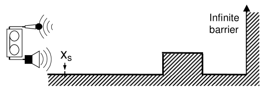
Figure 1: Schematic representation of the potential profile. The barrier height is set equal to $0.5V$ and is located between the sites $x_{s}+550a$ and $x_{s}+600a$.

Time-reversal via injection. In the following, we propose a gedanken scheme to achieve a perfect time-reversal of an arbitrary wave packet by assuming that a persistent non invasive injection and detection of waves at a single point is possible. In such conditions one would create an efficient stubborn daemon: the Perfect Inverse Filter (PIF). We illustrate this by considering an incoming wave packet in a semi-infinite space bounded by an infinite barrier at $x_{\max.}$which, together with a scattering barrier, define a reverberant region ( see Fig. 1). At the point $x_{s},$ located to the left of the scattering barrier, we alternate the use of an injector and a detector of wave function (probability and phase). This set up is a particular realization of the “sound Bazooka” scheme implemented by Fink’s group. However, instead of using the TRM, we proceed as follows:

1) We calculate the response of the system to an instantaneous excitation at site $x_{s}$ i.e. $G_{x_{s},x_{s}}^{R}(t)$ and compute its FT, $G_{x_{s},x_{s}}^{R}(\varepsilon)$.

2) We start with the empty cavity ( $\psi(x>x_{s},0)\equiv 0$) and a wave packet that travels towards it (e.g. a Gaussian centered at $x_{0}<x_{s}$). The probability density at time zero is shown in the top of the left panel of Fig. 2. It is followed by a sequence of snapshots of the density at selected times in the range $[0,2t_{R}]$ increasing from top to bottom and continuing in the right panel from bottom to top. The injection/detection point is indicated by a vertical dotted line in each panel.

3) During the period $(0,T_{rec}^{\mathrm{PIF}}=t_{R}-t_{1})$ the wave packet performs a free evolution: it enters to the cavity, collides with the barrier and then bounces back in the wall at the right end of the system and finally escapes towards the outer region at the left side. See left panel of Fig. 2. Provided that there are no localized states in the cavity and that the wave packet that escapes to the outer region does not return, the condition $\psi(x_{s},t>t_{R})\simeq 0$ can be fulfilled. During the whole period $T_{rec}^{\mathrm{PIF}}=t_{R}-t_{1}$ the wave function amplitude and phase at $x_{s}$ are registered. The range $(t_{1},t_{R})$ should contain the support of $\psi(x_{s},t),$ i.e. $\psi(x,t)\cong 0$ for $x>x_{s}$ and $t\notin(t_{1},t_{R}).$

4) Now our target function is $\psi_{rev}(x_{s},t_{R}+\delta t)=\psi^{\ast}(x_{s},t_{R}-\delta t)$ with $0\leq\delta t\leq T_{rec}^{\mathrm{PIF}},$ i.e. the wave packet with reversed evolution. Using the information registered in the previous step, we Fourier transform it

$$\psi_{rev}(x_{s,}\varepsilon)\simeq\int_{0}^{T_{rec}^{\mathrm{PIF}}}\psi^{\ast}(x_{s},t_{R}-\delta t)\exp[\tfrac{\mathrm{i}\varepsilon(t_{R}+\delta t)}{{\hbar}}]\mathrm{d}\delta t.$$ (8)

and normalize it according to Eq. (7). Transforming back to time we get the actual time dependent injection acting for a time $T_{rec}^{\mathrm{PIF}}$. The injection also produces a wave packet that travels to the left, i.e. escaping to the left outer region, see Fig. 2. Hence, perfect time reversion is restricted to the cavity, i.e. $x>x_{s}$.

5) After injection has seased, the original wave-packet is recovered at time $2t_{R}$ with an inverted momentum: this is the Loschmidt Echo. Figure 2 also shows, in dotted line, the echo resulting from TRM procedure [7], which in this case would require the recording only the outgoing wave described in step 3) which is time-reverted and reinjected without further procesing.

In Fig. 3, the density at site $x_{s}$ is shown at different times. The actual PIF density is plotted with a solid line while the injected density at each time is shown with a dashed line. Notice that the injection intensity has to provide a wave propagating toward both the cavity and outer region. We also show, with a dotted line, the density obtained from the TRM procedure. Note that this density also exhibits an Echo at time $2t_{R}$ but with a reduced amplitude as compared with the original signal. While the PIF and TRM densities differ in their magnitude, their shape in $[t_{R},2t_{R}]$ is remarkably simmilar. This indicates the stability of the TRM in the condition considered. We emphasize that by injecting probability amplitude according to Eq.(7) we exactly reverse the forward evolution of the initial wave packet. The correction imposed by the PIF procedure becomes non-trivial in cases where the incoming and outgoing signals superpose. In these cases the PIF procedure “filters” the outgoing portion as can be appreciated in Fig. 4. In the upper panel we display the forward evolution as registered at site $x_{s}$. In this case, one can roughly indentify three time regimes: entrance (IN), escape (OUT) and a Mixed region when both components interfere. The lower panel displays the time reversal procedure. The TRM would inject only the OUT portion of the registry shown in the upper panel. In contrast, the PIF procedure yields an injection that extends to the mixed region shown ligth grey shaded (yellow area on-line). The dark shaded (blue area on-line) PIF intensity constitutes a substantial improvement over the gray shaded (cyan area on-line) TRM signal.

The PIF protocol is valid for the reversal of any scalar waves as long as they satisfy a linear equation. Then, different propagators are described by the Green’s functions. The basic ingredients apply to elastic or electromagnetic waves [16] extending the range of applicability of the concepts introduced here.

The implementation of a stubborn Loschmidt daemon in a quantum system is not a simple task. However, standard pulsed NMR has the tools. In an ensemble of linear molecules, the interactions between nuclear spins can be manipulated [18] to obtain a polarization which is the square modulus of a single particle wave function or polarization amplitude [19] and constitutes a pseudo-pure state [17]. Detection at each time involves an ensemble measurement and a new experiment. In order to generate a local source/detector one resorts to the interaction between different nuclei, which can be engineered at will, e.g. a ¹³C  acts as such probe for a labeled ¹H. In fact, we have been able to inject a wave packet in a ¹H ring and follow its dynamics detecting simultanously the amplitude and relative phase at the labeled ¹H [20]. This is a double-slit like experiment that allows interferometry in the time domain [21]. If most of the polarization stays in the ¹³C, it is the small portion transfered to the proton system the one described by the theory above. While a full implementation of the quantum TRM or PIF requires setting many important experimental details, every step towards that goal would have potential use in spectral edition and quantum information processing. More immediately, classical wave systems, could benefit from our procedures which can be incorporated in a straightforward manner.

In summary, we have studied the Schrödinger equation with source boundary conditions. We have obtained a general solution for the inverse time problem which is expressed in terms of the Green’s function at the boundary region. Our results enabled us to develop the Perfect Inverse Filter protocol to implement a stubborn Loschmidt daemon. It allows one to achieve the perfect time reversal of the wave dynamics obtaining a Loschmidt Echo. In some cases, this protocol could improve the experimental procedure implemented with sound waves. Now that a perfect reversion can be obtained, a number of questions relevant to the Quantum Chaos field become pertinent related to the assestment of infidelity sources. On the view of the experimental results in sound waves [7], a stubborn daemon yields more robust results than its hasty counterpart. Hence, a whole field of study opens up.

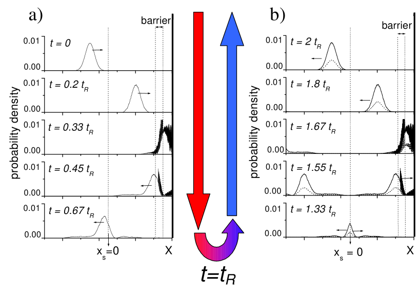
Figure 2: Distribution of probability density (in the cavity and outer region) for different times. Panel a) shows the forward evolution between $0$ and $t_{R}$. The backward evolution is shown in panel b). The solid line is the result of an appropriate injection, Eq. (7), while the dotted line is obtained by injecting only the time-reversed wave recorded at $x_{s}$ during the forward evolution. The initial gaussian wave packet, which is centered at $x_{s}-200a$, has $\sigma/a=50$ and $k_{0}a=1$.

Figure 3: Probability density at site $x_{s}$ as a function of time. The actual density (solid line) results from the injection of the density shown with a dashed line corresponding with the FT of Eq.(7). The density corresponding to the injection of the time-reversal of the recorded amplitude is also shown with a dotted line. The injection and recording periods, at site $x_{s}$, are specified in the top of the figure.

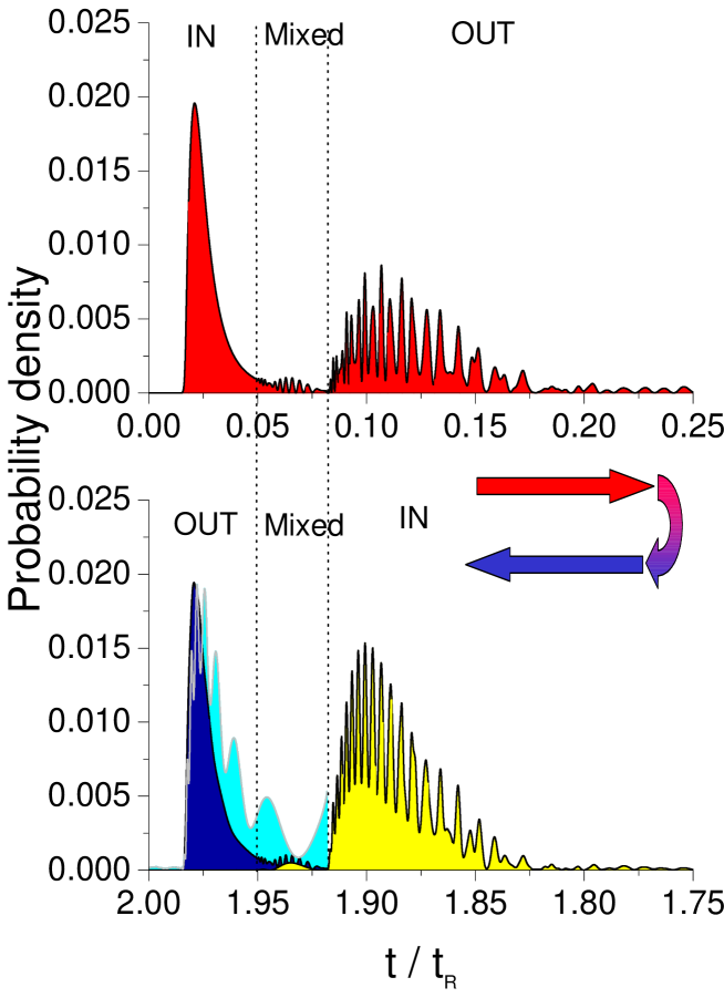
Figure 4: Upper panel: density at $x_{s}$ in a forward evolution of a wave packet. Lower panel: At rigth, the density injected at $x_{s}$ by the PIF procedure (shaded light-grey/yellow on-line) . Its evolution determines the correct reversed density (shaded dark/blue on line). The density obtained from TRM is shaded grey/cyan on-line. System parameters: Barrier height $0.2V$ between sites $x_{s}+100a$ and $x_{s}+105a$ and $x_{\max.}=200a.$ Gaussian wave packet centered at $x_{s}-100a$, with $\sigma/a=3$ and $k_{0}a=0.8$.

References

- [1] \NameWHEELER J. A. \BookPhysical Origins of Time Asymmetry \EditorHALLIWELL J. J., PÉREZ MERCADER J. and ZUREK W. H. \PublCambridge Univ. Press \Year1994 \Page1.
- [2] \NameKUHN T. S. \BookBlack-Body Theory and the Quantum Discontinuity \PublUniv. of Chicago Press \Year1987 \Page1894-1912.
- [3] HAHN E. L., Phys. Rev. 80 (1950) 580; BREWER R. G. and HAHN E. L., Sci. Am. 42 (Dec. 1984).
- [4] RHIM W. K., PINES A. and WAUGH J. S., Phys. Rev. Lett. 25 (1971) 218; ZHANG S., MEIER B. H. and ERNST R. R., Phys. Rev. Lett. 69 (1992) 2149.
- [5] USAJ G., PASTAWSKI H. M. and LEVSTEIN P.R., Mol. Phys. 95 (1998) 1229; PASTAWSKI H. M., LEVSTEIN P.R., USAJ G., RAYA J., HIRSCHINGER J., Physica A 283 (2000) 166.
- [6] JALABERT R. A. and PASTAWSKI H. M., Phys. Rev. Lett. 86 (2001) 2490.
- [7] FINK M., Phys. Scripta, T90 (2001) 268; TOURIN A., DERODE A., FINK M., Phys. Rev. Lett. 87 (2001) 274301.
- [8] CASSEREAU D. and FINK M., IEEE Trans. Ultrason. Ferroelec. and Freq. Contr. 39 (1992) 579.
- [9] EDELMAN G. F., AKAL T., HODKISS W. S., KIM S., KUPERMAN W. A., SONG H. C., IEEE J. Ocean Eng. 27 (2002) 602.
- [10] FINK M., MONTALDO G. and TANTER M., Annual Rev. Biomed. Eng. 5 (2003) 465.
- [11] MÜLLER L., KUMAR A., BAUMANN T. and ERNST R. R., Phys. Rev. Lett. 32 (1974) 1402.
- [12] VAN WILLIGEN H., LEVSTEIN P.R. and EBERSOLE M., Chem. Rev . 93 (1993) 173; ZEWAIL A. H., J. Phys. Chem. A. 104 (2000) 5660.
- [13] PASTAWSKI H. M., Phys. Rev. B 46, 4053 (1992).
- [14] ALLCOCK G. R., Ann. of Phys. 53 (1969) 253.
- [15] BAUTE A. D., EGUSQUIZA I. L. and MUGA J. G., J. Phys. A 34 (2001) 4289.
- [16] MOUSTAKAS A. L., BARANGER H. U., BALENTS L., SENGUPTA A. M. and SIMON S. H., Science, 287 (2000) 287.
- [17] DANIELI E. P., PASTAWSKI H. M. and LEVSTEIN P. R., Chem. Phys. Lett. 384 (2004) 306.
- [18] MÁDI Z. L., BRUTSCHER B., SCHULTE-HERBRÜGGEN T., BRÜSCHWEILLER R. and ERNST R. R., Chem. Phys. Lett. 268 (1997) 300.
- [19] PASTAWSKI H. M., LEVSTEIN P. R. and USAJ G., Phys. Rev. Lett. 75 (1995) 4310.
- [20] LEVSTEIN P. R., USAJ G. and PASTAWSKI H. M., J. Chem. Phys. 108 (1998) 2718.
- [21] PASTAWSKI H. M., USAJ G. and LEVSTEIN P. R., Chem. Phys. Lett. 261 (1996) 329.