Dynamical entanglement-transfer for quantum information networks

Abstract

A key element in the architecture of a quantum information processing network is a reliable physical interface between fields and qubits. We study a process of entanglement transfer engineering, where two remote qubits respectively interact with entangled two-mode continuous variable (CV) field. We quantify the entanglement induced in the qubit state at the expenses of the loss of entanglement in the CV system. We discuss the range of mixed entangled states which can be obtained with this set-up. Furthermore, we suggest a protocol to determine the residual entangling power of the light fields, inferring, thus, the entanglement left in the field modes which, after the interaction, are no longer in a Gaussian state. Two different set-ups are proposed: a cavity-QED system and an interface between superconducting qubits and field modes. We address in details the practical difficulties inherent in these two proposals, showing that the latter is promising under many aspects.

I Introduction

Distributed networks for quantum communication and quantum computation have recently received large attention being a promising architecture for quantum information processing. Efficient sources of entangled continuous variable (CV) states of light are readily available and field modes can act as reliable information carriers. On the other hand, it is more handy to manipulate the information stored in qubits embodied in atomic or solid-state systems. In many of the protocols for quantum information processing designed for distributed networks, entanglement plays a crucial role in establishing an exploitable quantum channel between two distant nodes eisert . This motivates the attempt to study and implement a reliable physical interface between fields and qubits. An interface allows for the transfer of information from the carrier to the qubit subsystem. In this context, it is interesting to consider the ability of a quantum-correlated two-mode field to induce entanglement in several different qubit subsystems.

On the other hand, under a more fundamental point of view, an analysis of the entangling power of a correlated two-mode state can be a useful tool to indirectly quantify the entanglement left between the modes after the interaction with a given pair of qubits. For a non-Gaussian field state, in particular, there is a lack of objective criteria to determine whether or not entanglement is present between two modes. We show that the capability of the light fields to induce entanglement in two initially separable qubits provides a test for the inseparability of the fields.

The implementation of such a physical interface, thus, opens a way to investigate the exchange of entanglement between systems defined in heterodimensional Hilbert spaces wonmin ; kraus ; mauro and to the entanglement transfer processes, where entanglement increases in one system at the expense of the loss of the other one, through their interaction.

In this work, we study a two-qubit system interacting with a quantum-correlated two-mode squeezed state of light through bi-local resonant interactions. The system we analyze allows to engineer entanglement transfer, generating qubit states with a controllable amount of entanglement. We show that it is actually possible to explore a large part of the space of the entangled mixed states (EMS) of two qubits, including the class of boundary states having the maximum amount of entanglement for a given value of the purity of the state munro1 . The generation of arbitrary and controllable entangled mixed states is relevant to investigate about the role that entanglement and purity have for the tasks of Quantum Information Processing (QIP). It has been proved, for example, that while entanglement is a fundamental requirement to efficiently perform the Shor’s factorization, purity is not parkerplenio . Moreover, in some cases, efficient QIP can be performed even relaxing the requirements, in terms of quantum correlations and purity, of a quantum channel. For example, a neat threshold exists for the allowed mixedness of an entangled mixed state to be usefully used in a teleportation protocol bosevedral .

The interest in the generation of EMS and in quantifying the entangling power of a given two-mode entangler leads us to look for practical implementations of the model we propose here. We consider two different set-ups to implement our model, namely a cavity-quantum electrodynamics (cavity-QED) system and Josephson charge qubits interfaced to field modes. We describe the two systems in some details and compare their performances. In the first proposal we consider two optical cavities, each interacting with one of the modes of a two-mode squeezed state of light respectively. After the squeezed state feeds the cavities, two two-level atoms cross their respective cavities. However, this set-up faces important practical difficulties. The cavity-photon lifetime turns out to be comparable to the operation times of our set-up, a feature that is typical of the weak coupling regime of the atom-field interaction. On the other hand, the advantages of a much stronger coupling buisson ; francescopino can be exploited in the second scenario we propose, where the qubits and the cavity are implemented by superconducting devices integrated on the same chip. In this case, flying qubits are no more required so that the control over the interaction times is easier. Moreover, in this scheme the qubit parameters can be independently modulated via external electric and magnetic fields Schon . The interaction can be controlled by tuning the qubit on/off resonance with a cavity mode francescopino ; mauro . A promising design of integrated superconducting qubit and cavity has been recently proposed schelkopf and the first experiments have already demonstrated a quality factor $Q>10^{4}$ for the cavity schelkopf-priv , which is enough to implement the protocols discussed in refs. francescopino ; mauro .

The paper is organized as follows. In Section II we describe the general scheme proposed here, introduce the space of the entangled mixed states of two qubits and show that our model allows for an extensive exploration of such a space. In Section III, we infer the correlations left between two field modes after the interaction. We propose a scheme that, extending the interaction model to more than a single qubit pair, allows to get some additional information on the residual entanglement capabilities of the field, bypassing the lack of a necessary and sufficient criterion for the entanglement of a non-Gaussian state. In Section IV, we describe the proposed implementations of our system. For a cavity-QED system, we discuss the effect of spectator atoms and of the cooperativity parameter turchettekimble . This kind of difficulties are no more present when Cooper pair boxes Schon integrated in high-quality transmission lines are used.

II The model of entanglement generation

We introduce the system we consider, based on the interaction of a pair of remote qubits with local environments that, for definiteness, we model as single bosonic modes, respectively. While the physical system that embodies the qubits will not be specified until necessary, this schematization perfectly matches the situation in which the two qubits are coupled to the field modes of two cavities. This assumption does not limit the generality of our approach allowing, on the other hand, to cover many different physical systems that are promising for the purposes of QIP massimolibro . We will consider explicitly this case, from now on. We are interested in a situation in which the field modes of the two cavities exhibit non-classical correlations and local interactions of each qubit with the respective cavity mode are arranged. A way in which this can be achieved is sketched in Fig. 1.

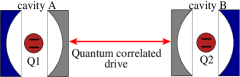
Figure 1: Two remote cavities are driven by a quantum correlated two-mode field. We explicitly consider the case of a two-mode squeezed driving field coupled to each cavity via a leaky mirror and preparing a quantum-correlated two-mode state of the cavity fields. After the preparation of the cavity field, local interactions with two generic (flying or static) qubits are arranged.

In details: two remote but identical cavities are initially prepared in their vacuum states. One mirror of each cavity is assumed to be perfect while the other has non-zero transmittivity. The leaky mirror is coupled to one mode of an external two-mode squeezed state with coupling strength $\kappa$. The squeezed state of the two external modes $a$ and $b$ is represented by $\left|S\right\rangle_{ab}=(\cosh{r})^{-1}\sum^{\infty}_{n,0}(\tanh{r})^{n}\left|n\right\rangle_{a}\left|n\right\rangle_{b}$, where $\left\{\left|n\right\rangle\right\}_{a,b}$ are the Fock bases for the field modes, and $r$ is the squeezing parameter. If the coherence time of the driving field is shorter than $\kappa^{-1}$, we can treat the cavity mirror as a beam splitter continuously fed by squeezed fields myungimoto . The state of the cavity modes $A$ and $B$ evolves due to the coupling and is described by the reduced density matrix wonmin

$$\rho_{AB}=\mbox{Tr}_{ab}\left(\hat{{\cal B}}_{Aa}(\theta)\hat{{\cal B}}_{Bb}(\theta)\rho_{abAB}(0)\hat{{\cal B}}^{{\dagger}}_{Aa}(\theta)\hat{{\cal B}}^{{\dagger}}_{Bb}(\theta)\right)$$ (1)

$$=\hskip-3.0pt\sum^{\infty}_{n,m=0}\hskip-3.0pt\sum^{\min(n,m)}_{k,l=0}\hskip-3.0pt{\cal A}^{nm}_{kl}\left|n-k\right\rangle_{A}\!\left\langle m-k\right|\otimes\left|n-l\right\rangle_{B}\!\left\langle m-l\right|.$$

Here, $\hat{B}_{Aa}(\theta)=\exp\left[{\theta}(\hat{A}\hat{a}^{{\dagger}}-\hat{A}^{{\dagger}}\hat{a})\right]$ is the beam splitter operator barnett with its reflection coefficient $\sin\theta$ (basically determined by $\kappa$ myungimoto ), $\hat{a}$ ($\hat{a}^{\dagger}$) is the annihilation (creation) operator for the external field mode $a$ (analogously for field mode $b$) while $\hat{A}$ ($\hat{A}^{\dagger}$) and $\hat{B}$ ($\hat{B}^{\dagger}$) are the bosonic operators of the cavity fields. We have defined ${\cal A}^{nm}_{kl}=\chi_{nm}G^{nm}_{kl}$, with $\chi_{nm}=(\tanh{r})^{n+m}/{(\cosh{r})}^{2}$ and $G^{nm}_{kl}=\prod^{m}_{\alpha=n}\prod^{l}_{\beta=k}\sqrt{\alpha{!}/[\beta{!}(\alpha-\beta)!]}(\cos\theta)^{\beta}(\sin\theta)^{\alpha-\beta}$. When the reflected part of the external field is minimized, a two-mode squeezed state quickly builds up inside the cavities. Note that a two-mode Gaussian field is built into the cavity, regardless of the coupling strength. This model is exactly the same as the initial field interacting with a zero-temperature reservoir myungimoto and it is known that entanglement can always be found during the evolution of an initial two-mode squeezed field in the zero-temperature vacuum duan .

After the cavity field is prepared, the interaction with a pair of qubits with logical states $\left|0\right\rangle_{i}$ and $\left|1\right\rangle_{i}$ ($i=1,2$) begins. Here, the interaction model is assumed to be of the resonant Jaynes-Cummings type jc . The interaction Hamiltonian for the cavity A is

$$\hat{H}_{A1}=\hbar\Omega\left(\hat{A}\left|1\right\rangle_{1}\!\left\langle 0\right|+\hat{A}^{\dagger}\left|0\right\rangle_{1}\!\left\langle 1\right|\right),$$ (2)

where $\Omega$ is the atom-field coupling constant. An analogous Hamiltonian describes the interaction between the second qubit and cavity B. Before entering the detail of protocols, we point out that the Hamiltonian we discuss can be also implemented by superconducting devices buisson ; francescopino ; schelkopf .

The interaction between cavity modes and qubits gives rise to an unitary evolution $\hat{U}_{A1}(t)\otimes\hat{U}_{B2}(t)$ of the whole system, where $\hat{U}_{A1}(t)=\exp(-i\hat{H}_{A1}t/\hbar)$. The effective evolution of the two qubits, on the other hand, is non-unitary and is described by the reduced density matrix $\rho_{12}(t)$ obtained by tracing out the cavity fields as $\rho_{12}(t)=\mbox{Tr}_{AB}\left(\hat{U}_{A1}(t)\otimes\hat{U}_{B2}(t)\rho_{12}(0)\otimes\rho_{AB}\hat{U}^{{\dagger}}_{A1}(t)\otimes\hat{U}^{{\dagger}}_{B2}(t)\right)$. Here, we consider the initial state $\rho_{12}(0)=\left|00\right\rangle_{12}\!\left\langle 00\right|$ commentoM and define the rescaled time of this first interaction $\tau_{1}=\Omega{t}$. In the basis $\left\{\left|11\right\rangle,\left|10\right\rangle,\left|01\right\rangle,\left|00\right\rangle\right\}_{12}$, $\rho_{12}(\tau_{1})$ takes the form

$$\rho_{12}(\tau_{1})=\begin{pmatrix}A&0&0&-D\\ 0&B&0&0\\ 0&0&C&0\\ -D&0&0&F\end{pmatrix},$$ (3)

with $F=1-A-B-C$,

$$\begin{split}&A=\sum^{\infty}_{n=0}\sum^{n}_{k,l=0}{\cal A}^{nn}_{kl}\sin^{2}(\tau_{1}\sqrt{n-k})\sin^{2}(\tau_{1}\sqrt{n-l}),\\ &B=\sum^{\infty}_{n=0}\sum^{n}_{k,l=0}{\cal A}^{nn}_{kl}\sin^{2}(\tau_{1}\sqrt{n-k})\cos^{2}(\tau_{1}\sqrt{n-l}),\\ &C=\sum^{\infty}_{n=0}\sum^{n}_{k,l=0}{\cal A}^{nn}_{kl}\cos^{2}(\tau_{1}\sqrt{n-k})\sin^{2}(\tau_{1}\sqrt{n-l}),\\ \end{split}$$ (4)

and the off-diagonal component given by

$$\begin{split}D&=\sum^{\infty}_{n=0}\sum^{n}_{k,l=0}{\cal A}^{nn+1}_{kl}\sin(\tau_{1}\sqrt{n-k+1})\\ &\times\cos(\tau_{1}\sqrt{n-k})\sin(\tau_{1}\sqrt{n-l+1})\cos(\tau_{1}\sqrt{n-l}).\\ \end{split}$$ (5)

In order to quantify the quantum correlations between the qubits after the interaction with the cavity modes, we use the negativity of the partially transposed density operator (NPT), which is a necessary and sufficient condition for entanglement of any bipartite qubit system zyczkowski . The entanglement measure based on NPT is defined as ${\cal E}_{NPT}=-2\lambda^{-}$, where $\lambda^{-}$ is the negative eigenvalue of the partially transposed density matrix $\rho^{PT}_{12}$ (here with respect to qubit $2$) leekim . In our case, $\lambda^{-}$ does not depend on the populations of states $\left|11\right\rangle_{12},\,\left|00\right\rangle_{12}$. Explicitly

$$\lambda^{-}=\frac{1}{2}\left\{{B}+C-\sqrt{4D^{2}+{\left(B-C\right)^{2}}}\right\}.$$ (6)

Figure 2: ${\cal E}_{NPT}$ versus the rescaled interaction time $\tau$ (in units of $\pi$). The squeezing parameter of the field is $r=0.26$ (full line), $r=0.86$ (stars), $r=1.2$ (full squares). These values offer a trade-off between the visibility of each curve and the insight given in the dynamics of the entanglement. We take $\sin^{2}\theta=0.1$.

In Fig. 2 we plot ${\cal E}_{NPT}$ versus $\tau_{1}$ for a reflectivity of the cavity $\sin^{2}\theta=0.1$ and three different values of the squeezing parameter $r$. The entanglement is peaked at $\tau_{1}=(2q+1)\pi/2$ ($q$ integer). For small values of $r$, the two-mode squeezed state can be approximated by $\left|00\right\rangle_{ab}+{r}\left|11\right\rangle_{ab}$ so that the qubit-field interaction results in $\left|00\right\rangle_{12}-{r}\left|11\right\rangle_{12}$ at $\tau_{1}=(2q+1)\pi/2$. However, as squeezing is increased, the Rabi oscillations become more complicated due to the importance of terms relative to higher photon numbers in eqs. (4) and (5). This reduces the qubit entanglement and makes ${\cal E}_{NPT}$ a non-monotonous function of the squeezing. This is explicitly shown in Fig. 2, for $r=1.2$ (full squares). In this case, the entanglement function is always below the curve relative to the smaller $r=0.86$ (stars) that allows for the maximum ${\cal E}_{NPT}$ at $\tau_{1}\approx{3\pi/2}$.

Another useful quantity to characterize the state of the qubits is the degree of purity of $\rho_{12}$. We have studied the behavior of the linearized entropy $S_{L}(\rho_{12})=(4/3)\left[1-Tr\left(\rho^{2}_{12}\right)\right]$, which gives a measure of the degree of mixedness for the state described by $\rho_{12}$ munro1 . $S_{L}(\rho_{12})$ ranges from $0$ (pure states) to $1$ (maximally mixed states). The linearized entropy can be studied as a function of $\tau_{1}$ and for different values of $r$. We have combined the temporal behavior of entanglement and linear entropy onto an entanglement-purity plane as shown in Fig. 3.

Figure 3: Navigation in the plane of the entangled mixed states of two qubits. We used $\sin^{2}\theta=0.1$. The measures for the entanglement and purity are negativity of partial transposition ${\cal E}_{NPT}$ and linearized entropy $S_{L}$. The curvilinear abscissa is $\tau_{1}\in[0,3\pi/2]$. We show the cases with $r=0.46$ (rhombuses), $r=0.86$ (stars) and $r=2$ (filled squares). The solid line is the MEMS boundary.

In this plot, each curve is relative to a specific value of the squeezing parameter, while each point along a curve gives the entanglement and purity of the corresponding state at a specific interaction time (so that $\tau_{1}$ represents a curvilinear abscissa, in this plot). The solid line is the upper bound to the region occupied by physically achievable mixed states for a given degree of entanglement ${\cal E}_{NPT}\geq{0}$. They are known as maximally entangled mixed states (MEMS) munro1 . A parameterization of MEMS is critically dependent on the chosen measures of entanglement and purity. If the negativity of partial transposition is taken, there are two classes of one-parameter states belonging to MEMS and giving the same boundary. The first class corresponds to the family of Werner states $\rho_{W}=p\left|\phi^{+}\rangle\langle\phi^{+}\right|+(1-p)\mbox{$1{\bf l}$}_{2\times 2}$, with $\left|\phi^{+}\right\rangle=(1/\sqrt{2})\left(\left|00\right\rangle+\left|11\right\rangle\right)$ and $0\leq{p}\leq 1$. The other class can be resented by

$$\rho_{MEMS}=\begin{pmatrix}\frac{1+\sqrt{1+3p^{2}}}{6}&0&0&\frac{p}{2}\\ 0&\frac{2-\sqrt{1+3p^{2}}}{3}&0&0\\ 0&0&0&0\\ \frac{p}{2}&0&0&\frac{1+\sqrt{1+3p^{2}}}{6}\end{pmatrix}.$$ (7)

Thus, the Werner states represent a frontier for the achievable amount of entanglement that a given mixed state can have. This feature is unique for the choice of NPT as the measure of entanglement munro1 .

Several interesting points can be addressed closely analysing Fig. 3. First of all, the interaction model described here is able to produce entangled, nearly pure, state of two qubits (see, for example, the last point on the curve relative to $r=0.46$) that can be used to test protocols for QIP bosevedral . As the value of $r$ increases, the states of the qubits get closer to the frontier curve of MEMS, even if the corresponding states are weakly entangled for longer periods of time. As was pointed out, this is due to the contribution of highly excited photon number states, in the Schmidt decomposition of a two-mode squeezed state $\left|S\right\rangle$, for larger values of $r$ wonmin . Our theoretical model is flexible enough to generate arbitrary entangled mixed states of two qubits up to the boundary-class of MEMS. Recently, theoretical and experimental efforts have been performed in the generation of these states using different mechanisms parkinskwiat . In our scheme, the local interactions with the two-mode entangler induces time-dependent quantum correlations between the qubits. The mixedness of the two-level systems state is due to their entanglement with the cavity modes. We will see that, in fact, the entanglement between the qubits is set at the expenses of the correlations between the field modes.

III Entanglement dynamics for cavity fields

In the previous section, we studied the amount of entanglement generated in a bipartite two-level system by the interaction with a two-mode squeezed state. Now, we turn our attention to the entanglement left between the cavity fields. After the interaction, the cavity fields state is given by

$$\hat{\rho}_{AB}(t)=\mbox{Tr}_{12}\left(\hat{U}_{AB12}(t){\rho}_{AB}(0)\otimes{\rho}_{12}(0)\hat{U}_{AB12}^{\dagger}(t)\right),$$ (8)

where $\hat{U}_{AB12}(t)=\hat{U}_{A1}(t)\otimes\hat{U}_{B2}(t)$. It is not difficult to see that the cavity field is no more Gaussian after the interaction.

Differently from the qubit case, how to quantify the quantum correlations of a CV state is only partially known. For the case of a Gaussian state, NPT can be used as a separability criterion as well as a measure of entanglement Simon ; DGCZ . In this case, the NPT condition for separability is equivalent to the violation of the uncertainty principle by a partially transposed density operator Simon . To study the uncertainty principle, it is useful to consider the vector of the field quadratures $\hat{\xi}=(\hat{q}_{1},\hat{p}_{1},\hat{q}_{2},\hat{p}_{2})^{T}$, where $\hat{q}_{1}=\left(\hat{A}+\hat{A}^{{\dagger}}\right)/\sqrt{2}$, $\hat{p}_{1}=-i\left(\hat{A}-\hat{A}^{{\dagger}}\right)/\sqrt{2}$ and $\hat{q}_{2},\,\hat{p}_{2}$ are analogously defined in terms of $\hat{B}$ and $\hat{B}^{{\dagger}}$. The field quadratures satisfy the commutation relations $[\hat{\xi}_{\alpha},\hat{\xi}_{\beta}]=i\Omega_{\alpha\beta}$, where $\Omega_{\alpha\beta}$ are the elements of the $4\times{4}$ matrix ${\bf\Omega}=\oplus^{2}{\bf J}$, with ${\bf J}=\begin{pmatrix}0&1\\ -1&0\end{pmatrix}$. Some of the statistical properties of a two-mode CV state can be inferred from the $4\times 4$ covariance matrix $\bf V$, defined by $V_{\alpha\beta}=\langle\Delta\hat{\xi}_{\alpha}\Delta\hat{\xi}_{\beta}+\Delta\hat{\xi}_{\beta}\Delta\hat{\xi}_{\alpha}\rangle/2$, with ${\Delta\hat{\xi}}_{\alpha}=\hat{\xi}_{\alpha}-\left\langle\hat{\xi}_{\alpha}\right\rangle$ and the expectation values evaluated over the state of the light fields. In terms of ${\bf V}$, the uncertainty relation for the field quadratures takes the form ${\bf V}+i{\bf\Omega}\geq 0$. Using the block representation ${\bf V}=\begin{pmatrix}{\bf A}&{\bf C}\\ {\bf C}^{T}&{\bf B}\end{pmatrix}$, with ${\bf A,B}$ and ${\bf C}$ $2\times{2}$ matrices, the uncertainty relation can be restated as Simon

$$\begin{split}\Delta&\equiv(\det{\bf A})(\det{\bf B})+\left({1}-\det{\bf C}\right)^{2}-\mbox{Tr}({\bf\tilde{A}}{\bf\tilde{C}}{\bf\tilde{B}}{\bf\tilde{C}}^{T})\\ &-(\det{\bf A}+\det{\bf B})\geq{0}.\end{split}$$ (9)

with ${\bf\tilde{A}}={\bf AJ}$, ${\bf\tilde{B}}={\bf BJ}$ and ${\bf\tilde{C}}={\bf CJ}$. Each term of $\Delta$ is invariant under local linear canonical transformations. Partial transposition is equivalent to a mirror reflection (that performs the transformation $\hat{p}_{i}\rightarrow-\hat{p}_{i}$) in the phase-space. This changes the sign of $\det{\bf C}$, leaving the other terms unaffected Simon . Thus the uncertainty $\Delta_{NS}$ for the partially transposed density matrix is obtained replacing ${\bf C}$ by $\left|\det{\bf C}\right|$ in Eq. (9). In our study, the function $\Delta_{NS}$ depends on the squeezing parameter $r$ and the interaction time $\tau_{1}$. For a Gaussian state, $\Delta_{NS}<0$ is a necessary and sufficient condition for entanglement.

For non-Gaussian states the situation is more complicated. The violation of the Heisenberg uncertainty relation by $\rho^{PT}_{AB}$ is only a sufficient condition for non-separability of the state. Nevertheless, as far as the authors are concerned, the uncertainty criterion is one of the most successful conditions to test entanglement of even a non-Gaussian state. We challenge this condition in the following.

In Fig. 4, $\Delta_{NS}$ for the cavity fields after the interaction with the qubits is plotted against $\tau_{1}$ for two significant values of the squeezing parameter. As done before, we assume the qubits initially prepared in their ground states $\left|00\right\rangle_{12}$. Interestingly, $\Delta_{NS}$ is negative for most of the interaction time, when $r=0.46$ (solid line). This means that the cavity field modes are in an entangled state even after the qubit-field interaction. The dynamics of $\Delta_{NS}$ is opposite to the qubit entanglement as it is apparent comparing Figs. 2 and 4. This behavior is consistent with the idea that the entanglement in the field is transferred to the qubits. On the other hand, for $r=0.86$ the entanglement induced between the qubits does not really match to the behavior of $\Delta_{NS}$ (dashed line).

Figure 4: This plot shows the dynamics of the uncertainty relation with partially transposed density matrix. Negative values show the violation of uncertainty or, equivalently, the non-separability of the cavity field modes $A$ and $B$ depending on the atom-field interaction time. We set $(\sin\theta)^{2}=0.1$ with $r=0.46$ (solid line) and $r=0.86$ (dotted line).

More informations about the entanglement of the field modes can be obtained testing their entangling power, that is their ability to set entanglement in an additional pair of initially separable qubits. In this case, if the cavity fields are not entangled there is no way to transfer correlations to two additional qubits. A nonzero entangling power is, thus, a condition for the fields states to be inseparable.

We let a second pair of qubits (indexed by 3 and 4) interact with the respective cavities for a time $\tau_{2}$. In general, the degree of entanglement ${\cal E}_{NPT,34}$ between the qubits depends also upon $\tau_{1}$, the interaction time with the first pair. In Fig. 5 we plot $\max_{\tau_{2}}{\cal E}_{NPT,34}(\tau_{1},\tau_{2})$, that is the maximum achievable entanglement ${\cal E}_{NPT,34}$ for a given interaction time $\tau_{1}$. We consider $r=0.86$ and all the qubits initially in their ground state. Obviously, if the first pair of qubits does not interact with the cavities ($\tau_{1}=0$), the entanglement settled in the second pair is the maximum achievable. Comparing Figs. 2 and 5, we note that the second pair may be entangled more as the first pair is entangled less and vice-versa. Notice that at $\tau\simeq{1.5}$, i.e. when the entanglement of the first pair is maximal (see Fig. 2), we find that ${\cal E}_{NPT,34}$ is nonzero, showing that even in this case the entanglement capability of the cavity fields is not exhausted by the first interaction. Thus the field modes in the cavities are still quantum-mechanically correlated and able to entangle the two qubits by the local interactions, despite the fact that $\Delta_{NS}$ is positive. In this example, the entanglement capability is a more powerful test for the entanglement of the cavity fields.

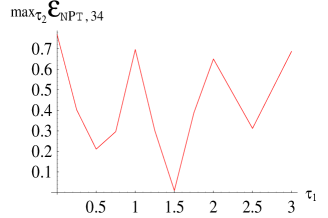
Figure 5: This plot shows the entanglement between qubits $3$ and $4$, maximized with respect to the interaction time $\tau_{2}$, as a function of $\tau_{1}$ (units of $\pi$). Because of the limit in computational power, the maximum of ${\cal E}_{NPT,34}$ is calculated for the cases of the first pair interaction times $\tau_{1}=n\pi/4$ (n=0,1,..,8).

IV Two physical implementations

The generation of two-qubit quantum states up to the MEMS boundary and the interest in inferring the entangling capabilities of a non-Gaussian CV state motivate the search for an implementation of the model studied so far. In this Section we describe two different proposals for a set-up: a cavity-QED scheme and an interface between superconducting charge qubits and cavity field modes. This latter, in particular, offers some intriguing perspectives in terms of coherence times and control of the qubits.

IV.1 Cavity-QED system

The first physical set-up we analyze is sketched in Fig. 6. As outlined in Section II, two remote one-sided optical cavities are initially prepared in the vacuum state. A two-mode squeezed state is coupled to each cavity via the leaky mirrors. In what follows, we assume a broad-band external source. We call $\Delta\omega_{ext}$ the band-width of the dyriving source. To consider the external field as an infinite band-width drive and use the (simple) analytical expressions valid for a broad-band squeezed state, the condition $\kappa\ll\Delta\omega_{ext}$ has to be fulfilled. However, it is typically $\Delta\omega_{ext}\lesssim{\kappa}$  turchettekimble . This means that to compare any theoretical prediction to the results of a real experiment, a more involved finite band-width approach must be used turchettekimble . This goes beyond the tasks of this work and we will assume the broad-band condition for our theoretical investigation. We assume the cavity fields build up as a two-mode squeezed state before the interactions with the qubits start.

The qubits are here embodied by two flying two-level atoms of their ground and excited states $\left|g\right\rangle_{i},\,\left|e\right\rangle_{i}$ ($i=1,2$) that pass through the respective cavities.

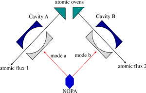
Figure 6: Two remote optical cavities are fed by the two-mode squeezed state generated by a nondegenerate-parametric-amplifier (NOPA). The external fields interact with two cavity modes via direct coupling to the leaky mirror of each cavity (the other being perfect). A low-density flux of two-level atoms, initially prepared in their ground states $\left|g\right\rangle$, passes through each cavity and interacts with the relevant cavity mode.

The behavior of a one-sided cavity, with respect to an external driving field, is influenced by the presence of an atomic medium. A two-level atom in a resonator can be seen as an intra-cavity lossy medium with a loss parameter proportional to the atomic cooperativity $C=\Omega^{2}/\kappa\Gamma$, where $\Gamma$ is the spontaneous emission rate from $\left|e\right\rangle$. For large $C$, the intra-cavity losses are so large that, eventually, no squeezed state builds up in the resonators turchettekimble . Realistic parameters, within the state of the art, are $(\kappa,\Omega,\Gamma)/2\pi=(80,40,4)\,MHz$. While the interaction of a cavity mode with the respective flying atom arises naturally in the form of a Jaynes-Cummings Hamiltonian, an important issue to take into account is the strength of this interaction. The optimal condition would be, obviously, the strong coupling regime $\Omega\gg\kappa,\Gamma$, where the coherent evolution of the atom-cavity system is faster than the decoherence mechanisms (dissipation, dephasing) due to the cavity decay and to the atomic spontaneous emission commento . In general strong coupling with flying atoms is a hard task to achieve, in optical systems commento2 . Furthermore, with the above values for $\kappa$, suitable for the external field to be injected, the field coherence times are within the range of $10\,nsec$. On the other hand, for cavity field waist of $\sim 10\,\mu{m}$ and an atomic velocity $\sim 300\,m/sec$ (that is an optimistic value) we get transit times in the range of $10\,nsec$, comparable to $\kappa^{-1}$. The dissipative effect due to the cavity decay is, thus, not negligible and experimental efforts are required to give a practical implementation of our scheme in this set-up. This has some implications for our method to infer the entangling capabilities of the fields by detecting the correlations between the atoms of a second pair. Intuitively, the time elapsing between the passages of two consecutive atoms has to be shorter than the life-time of a photon in an optical cavity. Otherwise, the decay of the cavity fields will destroy the quantum correlations between the field modes. The effects of the cavity decay can be described by introducing a dissipative term $\hat{H}_{loss}=-i\hbar\kappa\sum_{\alpha}\hat{\alpha}^{{\dagger}}\hat{\alpha}$ ($\alpha=A,B$) in the system Hamiltonian. This term gives an exponential decay (with rate $\kappa$) of the probability to find the cavity mode $\alpha$ in a Fock state with $p$ photons. We call $\bar{t}$ the time elapsing between the passage of the first and the second pair of qubits. It turns out that, for $\bar{t}$ equal to an atomic transit time (so that the first pair of atoms has surely left the region of interaction with the cavities), ${\cal E}_{NPT,34}$ is $50\%$ less than what we get in the ideal conditions. A way to minimize the elapsing time is to have the simultaneous presence of at least two qubits in the same cavity. For the sake of definiteness, we suppose the intensity of each cavity field to have a Gaussian radial profile centred at the cavity axis. We assume that, while the first atom is interacting with the cavity field, the second is at the border of the region of interaction and is weakly coupled to the field. We thus have a spectator atom inside the cavity turchettekimble . Usually, the spectator atoms give rise to additional loss mechanisms that become important once the density of the spectators is such that their collective coupling to the cavity mode is comparable to $\Omega$. A way to reduce these losses would be, then, to control a very low-density atomic beam.

Having fixed the interaction time (that can be finely controlled), a possible source of errors, in our model, is represented by the mismatched injection of the atoms in the cavity. The distribution of the atomic velocities is thermal and it is, in general, hard to arrange the simultaneous entrance of two atoms in two remote cavities. Obviously, a certain control is possible by means of atomic cooling techniques. However, a quantitative analysis of the effect of a mismatched triggering of the qubit-cavity mode interactions shows that the qubit-qubit entanglement is flattened to zero for times short compared to the interaction time $\tau_{1}$. The long-time behavior of ${\cal E}_{NPT,12}$, then, follows the pattern expected for a perfectly injected pair of qubits. In general, for a delay $\delta{t}$ between the entrance of $1$ and $2$ much smaller than $\Omega^{-1}$, this effect on the generation of a pair of entangled atoms is negligible. Obviously, a complete description of the effect of a mismatched atomic injection is given averaging the entanglement over $\delta{t}$. Such a detailed analysis is not necessary whenever we are able to keep the delay times within the condition $\delta{t}\ll\Omega^{-1}$. However, the control of $\delta{t}$ is per se a hard task. Some of the problems faced by this optical cavity-QED implementation can be solved in a scenario in which microwave cavities, interacting with long-lived Rydberg atoms, are considered. In this case, however, there is still the need for a fine control of the transit times and the simultaneous entrance of the atoms inside the cavities.

IV.2 Josephson qubits in a superconducting transmission line

We now consider a second class of implementations that combines some of the features of a microwave cavity-QED with the characteristics of a superconducting nano-circuit. The first advantage of a solid state device combined with quantum optics is the possibility of achieving a strong qubit-field mode Jaynes-Cummings type interaction buisson . This is basically due to the fact that the cavity field, in this case, is coupled to the charge of the qubit rather than its dipole. Various solid state implementations of the cavity have been proposed, ranging from large Josephson junctions buisson ; francescopino to superconducting films with large kinetic inductance buisson to microstrip resonators schelkopf . Several operational schemes for quantum protocols have been suggested, in this contexts super-cavity-th ; francescopino ; mauro . Coupling between a superconducting qubit in the charge regime Schon ; Nakamura and a classical Josephson junction has been implemented by the Saclay group vion . Decoherence of a qubit coupled with a quantum oscillator in the solid state has been studied in ref. francescopino . This analysis has revealed the existence of optimal operating conditions where decoherence is essentially due to spontaneous non-radiative decay of the qubit and leakage from the computational space of the cavity modes. This latter source of decoherence is minimized if the cavity is implemented by an integrated high-$Q$ microstrip resonator schelkopf so, in what follows, we will focus on this particular implementation.

In the proposal of ref. schelkopf , a Superconducting-Quantum-Interference-Device (SQUID) qubit Schon is placed between the planes of the resonator and the whole device is fabricated using nanolithographic techniques. The geometry of the resonator is such that a single mode of frequency $\sim{10}\,GHz$ can be accommodated. Microstrip transmission-lines having a $Q$ factor of about $10^{4}$ (corresponding to photon life-time of $0.1\mu{sec}$) have been already built and the effect of coupling with a qubit implemented by a SQUID has been demonstrated schelkopf-priv . Realistic estimates of the qubit life-time are in the range of some $\mu{sec}$ and the whole situation is reminding of a microwave cavity-QED set-up where the internal losses due to the cavity decay are very low. The source of quantum radiation can be built up using nondegenerate Josephson parametric amplifiers (in a distributed configuration, to limit the effects of gain-increasing noise). Microwave squeezed radiation (in a range of frequency of $\sim{10}\,GHz$) has been demonstrated and the source impedance-matched to superconducting lines used to transport the signals yurke .

A sketch of the set-up we consider is given in Fig. 7 (a). Let us first concentrate on the interaction of a SQUID qubit with a single cavity mode. We operate at the SQUID degeneracy point where the qubit is encoded in equally-weighted superpositions of states having zero and one excess Cooper-pair on the SQUID island, namely $\left|\pm\right\rangle=(1/\sqrt{2})\left(\left|0\right\rangle\pm\left|2e\right\rangle\right)$ ($2e$ being the charge of a Cooper pair). The free Hamiltonian of the SQUID is given by $H_{squid}=\frac{1}{2}E_{J}(\phi_{ext})\hat{\sigma}_{z}$. Here, $\hat{\sigma}_{z}$ is the $z$-Pauli operator and $E_{J}(\phi_{ext})$ is the Josephson energy which is tuned via an external magnetic flux $\phi_{ext}$ piercing the SQUID loop. This changes the energy separation between $\left|+\right\rangle$ and $\left|-\right\rangle$ and can be used to switch on/off resonance the interaction with the field mode. The degeneracy point is set by biasing the SQUID with a dc electric field via the ground plate of the resonator (Fig. 7 (a)). To quantify the strength of the qubit-field interaction, we model the cavity mode as a LC oscillator coupled to the SQUID as in Fig. 7 (b). The coupling is realized via the capacitor $C_{c}$. The interaction Hamiltonian can be cast in the form of a Jaynes-Cummings interaction with a Rabi frequency $\Omega$ that, for proper choices of the circuital parameters, is as large as ${0.5}\,GHz$ francescopino ; mauro . The strong coupling regime is thus possible in this set-up and interaction times of about $\sim 10\,nsec\ll\kappa^{-1},\Gamma^{-1}$ are enough to generate an entangled state of two qubits near to the MEMS boundary.

(a)                          (b)

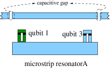
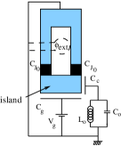
Figure 7: (a): Coupling between the field mode of a microstrip resonator and two SQUID qubits. We show just one resonator-qubits subsystem. This scheme has to be doubled considering a resonator $B$ interacting with qubits $2$ and $4$. Qubit $1$ and $2$ are used to generate a MEMS, while the interaction of the cavity modes with qubit $3$ and $4$ is useful to infer the state of the field modes. (b): Quantum circuit showing the LC-oscillator model (parameters $L_{0},\,C_{0}$) for the cavity mode. The coupling with the qubit is capacitive (coupling capacitance $C_{c}$). $C_{J_{0}}$ is the capacitance of each Josephson junction.

Two SQUID qubits (size $\sim\mu m$) can be easily accommodated in the cavity ($L\sim 1\,cm$) far enough to achieve negligible cross-talking (in principle due to direct capacitive and inductive coupling). Lithographic techniques allow to control (within few percent) the geometric characteristics and the resulting parameters of the device. The two qubits can be manipulated both simultaneously with a uniform magnetic field or independently with two separate coils. Due to charged impurities in the vicinity of the device, separate calibration at the degeneracy points is required for each qubit. This may be achieved with several adjustments of the design of ref. schelkopf , for instance by splitting the ground plate and by attaching a gate to each part.

The qubits have fixed position inside the cavities. This is an advantage with respect to common microwave cavity-QED systems, where flying atoms are required. The interaction times are regulated tuning the interaction between the SQUID and the cavity mode on and off resonance via $\phi_{ext}$. This avoids the problem of different qubit injections in the cavities even if the two SQUIDs have to be set on resonance with the respective cavity mode at the same time. The results we derived in Section IV.1 about a mismatched interaction-triggering are fully applicable here. On the other hand, having precisely fixed the number of qubits inside the cavities, we do not have to deal with spectator qubits.

We now briefly address the effect of decoherence in this set-up. Working at the charge degeneracy point, we minimize the effect of charge-coupled sources of noise francescopino . At this point, decoherence due to low-frequency modes vanishes at first order, a key property which allows to achieve coherence times of several hundreds of nanoseconds in the Saclay qubit vion . Furthermore, in our set-up, a selection rule prevents direct transitions between the states of the dressed doublet francescopino . As a result of this analysis, the performance-limiting process turns out to be the spontaneous decay from each state of the dressed doublet to the ground state. This results from comparable contributions of non-radiative decay of the qubit due to $1/f$ noise and losses due to the resonator. Life-times of $\sim 300\,ns$ were estimated for a system where the resonator is implemented by a Niobium Josephson junction. As we said, the losses of the resonator are further minimized in the proposal of ref. schelkopf , where $1/f$ noise is the ultimate limiting factor. Noise sources are switching charged impurities and their effect depends on statistical properties of the environment which are beyond the power spectrum elisabettalara . The actual dephasing rate depends also on details of the protocol and may show device-dependent features oneoverf . A detailed analysis with simulations of noisy gates for this device will be presented elsewhere falci . It is worth stressing here that, due to the qubit-resonator interaction, the energy levels of our qubit are much less sensitive to charge fluctuations than an isolated qubit at the optimal working point. This leads to a conservative estimate of coherence times in the range of $100\,ns$ falci , which surely allows for navigation and generation of MEMS.

At the degeneracy point, computational states of the qubit cannot be distinguished by measuring their charge. To detect the state of a SQUID qubit, we have to slowly shift the working point far from the degeneracy point, sweeping a dc-bias, to adiabatically transform the states of the qubit as $\left|+\right\rangle\rightarrow\left|2e\right\rangle,\,\left|-\right\rangle\rightarrow\left|0\right\rangle$. Then, charge measurements can be performed Nakamura .

As far as the interaction with more than one pair of qubits is concerned, we make use of the further degree of freedom represented by the tunability of the energy spacing between the levels of each qubit. We can proceed as follows. We suppose SQUID $1$ and $3$ in resonator $A$ (as in Fig. 7 (a)) while SQUID $2$ and $4$ interact with $B$. First, just $1$ and $2$ are resonant with the corresponding cavity mode while $3$ and $4$ are in a dispersive regime obtained either dc-biasing them or using an external magnetic flux. Once the interaction time $\tau_{1}$ has passed, we set the interaction with this pair in a dispersive regime while $3$ and $4$ are set on resonance with the respective cavity mode. The timing of these operation can be controlled electronically and the operating time can be as large as $50\,nsec$. In this condition, an entangled state of $3$ and $4$ is established still within the coherence time of the system.

In summary this second set-up offers some advantages with respect to a cavity-QED implementation. The most important points are related to the longer coherence times of the dynamical evolution while this is the main limitation of an optical set-up. An important problem for this solid state system is $1/f$ noise. In our opinion further improvements can be achieved by development of the design exploiting the possibilities of nanolithography.

V Conclusions

When a quantum-correlated CV state, such as a two-mode squeezed state of light, interacts with a bipartite two-dimensional system via bi-local interaction, effective entanglement transfer is possible. Theoretically, the state of the qubits can be engineered in terms of entanglement and purity. The model provides a tunable source of entangled mixed states that can be useful to investigate the interplay between entanglement and purity in QIP and for purposes of quantum communication and computation. The entangler, i.e. the CV system, does not exhaust its entangling capabilities with a single interaction but is able to entangle other pairs of qubits. This property can be exploited as a test, based on the entangling power of the field, for the quantum correlations in a non-Gaussian state of light.

We have proposed two different set-up in which this scheme can be implemented. The first is a cavity-QED system in which the qubits are embodied in two-level atoms crossing two optical cavities. The second proposal exploits the recent ideas about solid-state systems/quantum optics interfaces and uses superconducting qubits integrated in microstrip resonators. This second scenario, in particular, offers the advantages of a strong coupling regime of interaction (that is hard to get with optical cavities) without the difficulties connected with the management of flying qubits.

References

- (1) J. Eisert, K. Jacobs, P. Papadopoulos, M. B. Plenio, Phys. Rev. A 62, 52317 (2000); D. Collins, N. Linden, S. Popescu, Phys. Rev. A 64, 32302 (2001).
- (2) W. Son, M. S. Kim, J. Lee, D. Ahn, J. Mod. Opt. 49, 1739 (2002).
- (3) B. Kraus and J. I. Cirac, Phys. Rev. Lett. 92, 013602 (2004); M. Paternostro, W. Son, and M. S. Kim, quant-ph/0310031 (2003).
- (4) M. Paternostro, G. Falci, M. S. Kim, and G. M. Palma, quant-ph/0307163 (2003).
- (5) T.-C. Wei, K. Nemoto, P. M. Goldbart, P. G. Kwiat, W. J. Munro, F. Verstraete, Phys. Rev. A 67, 022110 (2003).
- (6) S. Parker and M. B. Plenio, Phys. Rev. Lett. 85, 3049 (2000).
- (7) S. Bose and V. Vedral, Phys. Rev. A 61, 040101(R) (2000).
- (8) O. Buisson and F.W.J. Hekking, in Macroscopic Quantum Coherence and Quantum Computing, D.V. Averin, B. Ruggero and P. Silvestrini Eds., Kluver (New York, 2001); O. Buisson, F. Balestro, J. P. Pekola, and F. W. J. Hekking, Phys. Rev. Lett. 90, 238304 (2003).
- (9) F. Plastina and G. Falci, Phys. Rev. B 67, 224514 (2003).
- (10) Y. Makhlin, G. Schön, A. Shnirman, Rev. Mod. Phys. 73, 357 (2001) and references within; M. Tinkham, Introduction to Superconductivity (McGraw-Hill International Editions, 1996).
- (11) S. M. Girvin, R.-S. Huang, A. Blais, A. Wallraff, and R. J. Schoelkopf, quant-ph/0310670 (2003).
- (12) D. Vion (private communication).
- (13) Q. A. Turchette, N. Ph. Georgiades, C. J. Hood, H. J. Kimble, and A. S. Parkins, Phys. Rev. A 58, 4056 (1998).
- (14) C. Macchiavello, G. M. Palma, and A. Zeilinger, Quantum computation and quantum information theory, (Singapore: World Scientific), 2001.
- (15) M. S. Kim and N. Imoto, Phys. Rev. A 52, 2401 (1995).
- (16) S. M. Burnett and P. M. Radmore, Methods in Theoretical Quantum Optics (Oxford Univ. Press, 1997).
- (17) J. Lee, M.S. Kim and H. Jeong, Phys. Rev. A 62, 032305 (2000).
- (18) E. T. Jaynes, and F. W. Cummings, Proc. IEEE 51, 89 (1963).
- (19) This state is known to offer some advantages in terms of the amount of entanglement that can be transferred from the field modes to the qubits mauro .
- (20) A. Peres, Phys. Rev. Lett. 77 1413 (1996); M. Horodecki, P. Horodecki, R. Horodecki, Phys. Lett. A 223, 1 (1996).
- (21) J. Lee, M. S. Kim, Y. J. Park and S. Lee, J. Mod. Opt. 47, 2151 (2000). 022110 (2003).
- (22) S. G. Clark and A. S. Parkins, Phys. Rev. Lett. 90, 047905 (2003); N. A. Peters, J. B. Altepeter, D. A. Branning, E. R. Jeffrey, T.-C. Wei, and P. G. Kwiat quant-ph/0308003 (2003).
- (23) R. Simon, Phys. Rev. Lett. 84, 2726 (2000).
- (24) L.-M. Duan, G. Giedke, J. I. Cirac, and P. Zoller, Phys. Rev. Lett. 84, 2722 (2000).
- (25) The spontaneous emission by the qubits can be included considering the non-Hermitian term in the energy of each qubit, being the spontaneous emission rate from . The effect of this term is a decay of with a rate dependent on .
- (26) The strong coupling regime has been recently achieved, for example, by McKeever et al., Nature 425, 268 (2003). In this case, however, a single atom trapped inside an optical resonator was considered.
- (27) F. Marquardt and C. Bruder, Phys. Rev. B 63, 054514 (2001); A. Blais and A.-M. S. Tremblay, Phys. Rev. A 67, 012308 (2003).
- (28) Y. Nakamura, Yu. A. Pashkin, J. S. Tsai, Nature 398, 786 (1999).
- (29) D. Vion, A. Aassime, A. Cottet, P. Joyez, H. Pothier, C. Urbina, D. Esteve, M. H. Devoret, Science 296, 886 (2002).
- (30) B. Yurke, R. Movshovich, P. G. Kaminsky, P. Bryant, A. D. Smith, A. H. Silver, R. W. Simon, IEEE Trans. Magn. 27, 3374 (1991) and references within.
- (31) E. Paladino, L. Faoro, G. Falci, and R. Fazio, Phys. Rev. Lett. 88, 228304 (2002).
- (32) G. Falci, E. Paladino, R. Fazio, in Quantum Phenomena of Mesoscopic Systems, B.L. Altshuler and V. Tognetti Eds., Proc. of the International School “Enrico Fermi”, Varenna 2002, IOS Press (2004), cond-mat/0312550 (2003); Y. M. Galperin, B. L. Altshuler, D. V. Shantsev, in Proc. of NATO/Euresco Conf. ”Fundamental Problems of Mesoscopic Physics: Interactions and Decoherence”, Granada, Spain, Sept.2003; G. Falci et al. (in preparation).
- (33) G. Falci et al., Proc. of the Workshop MS+S2004 (in preparation).