Graph-based simulation of quantum computation in the density matrix representation

Abstract

Quantum-mechanical phenomena are playing an increasing role in information processing, as transistor sizes approach the nanometer level, and quantum circuits and data encoding methods appear in the securest forms of communication. Simulating such phenomena efficiently is exceedingly difficult because of the vast size of the quantum state space involved. A major complication is caused by errors (noise) due to unwanted interactions between the quantum states and the environment. Consequently, simulating quantum circuits and their associated errors using the density matrix representation is potentially significant in many applications, but is well beyond the computational abilities of most classical simulation techniques in both time and memory resources. The size of a density matrix grows exponentially with the number of qubits simulated, rendering array-based simulation techniques that explicitly store the density matrix intractable. In this work, we propose a new technique aimed at efficiently simulating quantum circuits that are subject to errors. In particular, we describe new graph-based algorithms implemented in the simulator QuIDDPro/D. While previously reported graph-based simulators operate in terms of the state-vector representation, these new algorithms use the density matrix representation. To gauge the improvements offered by QuIDDPro/D, we compare its simulation performance with an optimized array-based simulator called QCSim. Empirical results, generated by both simulators on a set of quantum circuit benchmarks involving error correction, reversible logic, communication, and quantum search, show that the graph-based approach far outperforms the array-based approach.

1 INTRODUCTION

Practical information-processing applications that exploit quantum-mechanical effects are becoming common. For example, MagiQ Technologies markets a quantum communications device that detects eavesdropping attempts and prevents them[19]. The act of eavesdropping can be modeled as both making a quantum measurement and corruption by environmental noise[15]. Additionally, quantum computational algorithms have been discovered to quickly search unstructured databases[10] and to factor numbers in polynomial time.[17] Implementing quantum algorithms has proved to be particularly difficult, however, in part due to errors caused by the environment[11, 14, 15]. Another related application is reversible logic circuits. Since the operations performed in quantum computation must be unitary, they are all invertible and allow re-derivation of the inputs given the outputs.[15] This phenomenon gives rise to a host of potential applications in fault-tolerant and low-power computation. Since reversible logic, quantum communication, and quantum algorithms can be modeled as quantum circuits[15], quantum circuit simulation incorporating errors could be of major benefit to these applications. In fact, any quantum-mechanical phenomenon with a finite number of states can be modeled as a quantum circuit[5, 15], which may lead to other design applications for quantum circuit simulation in the future.

We present a new technique that facilitates efficient simulation of the density matrix representation of quantum circuits. The density matrix representation is crucial in capturing interactions between quantum states and the environment, such as noise. In addition to the standard set of operations required to simulate with the state-vector model, including matrix multiplication and the tensor product, simulation with the density matrix model requires the outer product and the partial trace. The outer product is used in the initialization of qubit density matrices, while the partial trace allows a simulator to differentiate qubit states coupled to noisy environments or other unwanted states. The partial trace is invaluable in error modeling since it facilitates descriptions of single qubit states that have been affected by noise and other phenomena.[15]

Unfortunately, like the state-vector model, simulation with the density matrix is computationally challenging on classical computers. The size of any density matrix grows exponentially with the number of qubits or quantum states it represents.[15] Thus, simulation techniques which require explicit storage of the density matrix in a series of arrays are inefficient and generally intractable. However, the new simulation technique we propose is founded in graph-based algorithms which can represent and manipulate density matrices very efficiently in many important cases. A key component of our algorithms is the Quantum Information Decision Diagram (QuIDD) data structure, which can represent and manipulate a useful class of matrices and vectors commonly found in quantum circuit applications using time and memory resources that are polynomial in the number of qubits[22, 21]. A limitation of our previous QuIDD algorithms, and other graph-based techniques[9], is that they simulate the state-vector representation of quantum circuits. In this work, we present new algorithms to perform the outer product and the partial trace with QuIDDs. These algorithms enable QuIDD-based simulation of quantum circuits with the density matrix representation.

We also describe a set of quantum circuit benchmarks that incorporate errors, error correction, reversible logic, communication, and quantum search. To empirically evaluate the improvements offered by our new technique, we use these benchmarks to compare QuIDDPro/D with an optimized array-based density matrix simulator called QCSim.[4] Performance data from both simulators show that our new graph-based algorithms far outperform the array-based approach.

The paper is organized as follows. Section 2 provides background on decision diagram data structures and previous simulation work. In Section 3 we present our new algorithms along with a description of the QuIDDPro/D simulator. Section 4 describes the quantum circuit benchmarks and presents performance results on each benchmark for QuIDDPro/D and QCSim. Finally, in Section 5 we present our conclusions and ideas for future work.

2 BACKGROUND AND PREVIOUS WORK

The simulation technique proposed in this work relies on the QuIDD data structure, which is a type of graph called a decision diagram. This section presents the basic concepts of decision diagrams, assuming only a rudimentary knowledge of computational complexity and graph theory. It then reviews previous research on simulating quantum circuits.

2.1 Binary Decision Diagrams

Many decision diagrams are ultimately based on the binary decision diagram (BDD). The BDD was developed by Lee in 1959 in the context of classical logic circuit design.[12] This data structure represents a Boolean function $f(x_{1},x_{2},...,x_{n})$ by a directed acyclic graph (DAG) as shown in Fig. 1. By convention, the top node of a BDD is labeled with the name of the function $f$ represented by the BDD. Each variable $x_{i}$ of $f$ is associated with one or more nodes, each of which have two outgoing edges labeled then (solid line) and else (dashed line). The then edge of node $x_{i}$ denotes an assignment of logic $1$ to the $x_{i}$, while the else edge denotes an assignment of logic $0$. These nodes are called internal nodes and are labeled by the corresponding variable $x_{i}$. The edges of the BDD point downward, implying a top-down assignment of values to the Boolean variables depicted by the internal nodes.

At the bottom of a BDD are terminal nodes containing the logic values $1$ or $0$. They denote the output value of the function $f$ for a given assignment of its variables. Each path through the BDD from top to bottom represents a specific assignment of 0-1 values to the variables $x_{1},x_{2},...,x_{n}$ of $f$, and ends with the corresponding output value $f(x_{1},x_{2},...,x_{n})$.

$f=x_{0}\cdot x_{1}+x_{1}$
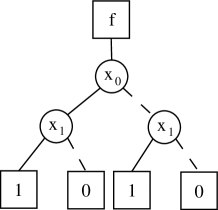
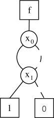
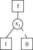
(a)	(b)	(c)	(d)

Figure 1: (a) A logic function, (b) its BDD representation, (c) its BDD representation after applying the first reduction rule, and (d) its ROBDD representation.

The memory complexity of the original BDD data structure conceived by Lee is exponential in the number of variables for a given logic function. Simulation of many practical logic circuits with this data structure was therefore impractical. To address this limitation, Bryant developed the Reduced Ordered BDD (ROBDD) [6], where all variables are ordered, and assignment of values to variables are made in that order. A key advantage of the ROBDD is that variable-ordering facilitates an efficient implementation of reduction rules that automatically eliminate redundancy from the basic BDD representation. These rules are summarized as follows:

1. There are no nodes $v$ and $v^{\prime}$ such that the subgraphs rooted at $v$ and $v^{\prime}$ are isomorphic

2. There are no internal nodes with then and else edges that both point to the same node

An example of how the rules distinguish an ROBDD from a BDD is shown in Fig. 1. The subgraphs rooted at the $x_{1}$ nodes in Fig. 1b are isomorphic. By applying the first reduction rule, the BDD in Fig. 1b becomes the BDD in Fig. 1c. Note that, in Fig. 1c, the then and else edges of the $x_{0}$ node now point to the same node. Applying the second reduction rule eliminates the $x_{0}$ node, resulting in the ROBDD in Fig. 1d. Intuitively it makes sense to eliminate the $x_{0}$ node since the output of the original function is determined solely by the value of $x_{1}$. In many Boolean functions, this type of redundancy is eliminated with varying success depending on the order in which variables in the function are evaluated. Finding the optimal variable ordering is an $NP$-complete problem, but efficient ordering heuristics have been developed for specific applications. Moreover, it turns out that many practical logic functions have ROBDD representations that are polynomial (or even linear) in the number of input variables [6]. Consequently, ROBDDs have become indispensable tools in the design and simulation of classical logic circuits.

2.2 BDD Operations

Even though the ROBDD is often quite compact, efficient algorithms are also needed to manipulate ROBDDs for circuit simulation. Thus, in addition to the foregoing reduction rules, Bryant introduced a variety of ROBDD operations with complexities that are bounded by the size of the ROBDDs being manipulated [6]. Of central importance is the $Apply$ operation, which performs a binary operation with two ROBDDs, producing a third ROBDD as the result. It can be used, for example, to compute the logical $AND$ of two functions. $Apply$ is implemented by a recursive traversal of the two ROBDD operands. For each pair of nodes visited during the traversal, an internal node is added to the resultant ROBDD using the three rules depicted in Fig. 2. To understand the rules, some notation must be introduced. Let $v_{f}$ denote an arbitrary node in an ROBDD $f$. If $v_{f}$ is an internal node, $Var(v_{f})$ is the Boolean variable represented by $v_{f}$, $T(v_{f})$ is the node reached when traversing the then edge of $v_{f}$, and $E(v_{f})$ is the node reached when traversing the else edge of $v_{f}$.

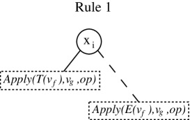
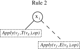
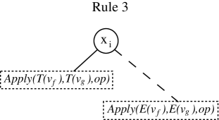
$x_{i}\prec x_{j}$	$x_{i}\succ x_{j}$	$x_{i}=x_{j}$

Figure 2: The three recursive rules used by the $Apply$ operation which determine how a new node should be added to a resultant ROBDD. In the figure, $x_{i}=Var(v_{f})$ and $x_{j}=Var(v_{g})$. The notation $x_{i}\prec x_{j}$ is defined to mean $x_{i}$ precedes $x_{j}$ in the variable ordering.

Clearly the rules depend on the variable ordering. To illustrate, consider performing $Apply$ using a binary operation $op$ and two ROBDDs $f$ and $g$. $Apply$ takes as arguments two nodes, one from $f$ and one from $g$, and the operation $op$. This is denoted as $Apply(v_{f},v_{g},op)$. $Apply$ compares $Var(v_{f})$ and $Var(v_{g})$ and adds a new internal node to the ROBDD result using the three rules. The rules also guide $Apply$’s traversal of the then and else edges (this is the recursive step). For example, suppose $Apply(v_{f},v_{g},op)$ is called and $Var(v_{f})\prec Var(v_{g})$. Rule 1 is invoked, causing an internal node containing $Var(v_{f})$ to be added to the resulting ROBDD. Rule 1 then directs the $Apply$ operation to call itself recursively with $Apply(T(v_{f}),v_{g},op)$ and $Apply(E(v_{f}),v_{g},op)$. Rules 2 and 3 dictate similar actions but handle the cases when $Var(v_{f})\succ Var(v_{g})$ and $Var(v_{f})=Var(v_{g})$. To recurse over both ROBDD operands correctly, the initial call to $Apply$ must be $Apply(Root(f),Root(g),op)$ where $Root(f)$ and $Root(g)$ are the root nodes for the ROBDDs $f$ and $g$.

The recursion stops when both $v_{f}$ and $v_{g}$ are terminal nodes. When this occurs, $op$ is performed with the values of the terminals as operands, and the resulting value is added to the ROBDD result as a terminal node. For example, if $v_{f}$ contains the value logical $1$, $v_{g}$ contains the value logical $0$, and op is defined to be $\oplus$ ($XOR$), then a new terminal with value $1\oplus 0=1$ is added to the ROBDD result. Terminal nodes are considered after all variables are considered. Thus, when a terminal node is compared to an internal node, either Rule 1 or Rule 2 will be invoked depending on which ROBDD the internal node is from.

The success of ROBDDs in making a seemingly difficult computational problem tractable in practice led to the development of ROBDD variants outside the domain of logic design. Of particular relevance to this work are Multi-Terminal Binary Decision Diagrams (MTBDDs) [7] and Algebraic Decision Diagrams (ADDs) [2]. These data structures are compressed representations of matrices and vectors rather than logic functions, and the amount of compression achieved is proportional to the frequency of repeated values in a given matrix or vector. Additionally, some standard linear-algebraic operations, such as matrix multiplication, are defined for MTBDDs and ADDs. Since they are based on the $Apply$ operation, the efficiency of these operations is proportional to the size in nodes of the MTBDDs or ADDs being manipulated. Further discussion of the MTBDD and ADD representations is deferred to Sec. 3 where the general structure of the QuIDD is described.

2.3 Previous Simulation Techniques

Quantum circuit simulators must support linear-algebraic operations such as matrix multiplication, the tensor product, and the projection operators. Simulation with the density matrix model additionally requires the outer product and partial trace.[15] Many simulators typically employ array-based methods to facilitate these operations and so require exponential computational resources in the number of qubits. Such methods are often insensitive to the actual values stored, and even sparse-matrix storage offers little improvement for quantum operators with no zero matrix elements, such as Hadamard operators. Previous work on these and other simulation techniques are reviewed in this subsection.

One popular array-based simulation technique is to simulate $k$-input quantum gates on an $n$-qubit state-vector ($k\leq n$) without explicitly storing a $2^{n}\times 2^{n}$-matrix representation.[16, 4] The basic idea is to simulate the full-fledged matrix-vector multiplication by a series of simpler operations. To illustrate, consider simulating a quantum circuit in which a $1$-qubit Hadamard operator is applied to the third qubit of the state-space $|00100\rangle$. The state-vector representing this state-space has $2^{5}$ elements. A naive way to apply the $1$-qubit Hadamard is to construct a $2^{5}\times 2^{5}$ matrix of the form $I\otimes I\otimes H\otimes I\otimes I$ and then multiply this matrix by the state-vector. However, rather than compute $(I\otimes I\otimes H\otimes I\otimes I)|00100\rangle$, one can simply compute $|00\rangle\otimes H|1\rangle\otimes|00\rangle$, which produces the same result using a $2\times 2$ matrix $H$. The same technique can be applied when the state-space is in a superposition, such as $\alpha|00100\rangle+\beta|00000\rangle$. In this case, to simulate the application of a $1$-qubit Hadamard operator to the third qubit, one can compute $|00\rangle\otimes H(\alpha|1\rangle+\beta|0\rangle)\otimes|00\rangle$. As in the previous example, a $2\times 2$ matrix is sufficient.

While the above method allows one to compute a state space symbolically, in a realistic simulation environment, state-vectors may be much more complicated. Shortcuts that take advantage of the linearity of matrix-vector multiplication are desirable. For example, a single qubit can be manipulated in a state-vector by extracting a certain set of two-dimensional vectors. Each vector in such a set is composed of two probability amplitudes. The corresponding qubit states for these amplitudes differ in value at the position of the qubit being operated on but agree in every other qubit position. The two-dimensional vectors are then multiplied by matrices representing single qubit gates in the circuit being simulated. We refer to this technique as qubit-wise multiplication because the state-space is manipulated one qubit at a time. Obenland implemented a technique of this kind as part of a simulator for quantum circuits [16]. His method applies one- and two-qubit operator matrices to state vectors of size $2^{n}$. Unfortunately, in the best case where $k=1$, this only reduces the runtime and memory complexity from $O(2^{2n})$ to $O(2^{n})$, which is still exponential in the number of qubits.

Another implicit limitation of Obenland’s implementation is that it simulates with the state-vector representation only. The qubit-wise technique has been extended, however, to enable density matrix simulation by Black et al. and is implemented in NIST’s QCSim simulator.[4] As in its predecessor simulators, the arrays representing density matrices in QCSim tend to grow exponentially. The drawbacks of this asymptotic bottleneck are demonstrated experimentally in Sec. 4.

Gottesman developed a simulation method involving the Heisenberg representation of quantum computation which tracks the commutators of operators applied by a quantum circuit [8]. With this model, the state need not be represented explicitly by a state-vector or a density matrix because the operators describe how an arbitrary state-vector would be altered by the circuit. Gottesman showed that simulation based on this model requires only polynomial memory and runtime on a classical computer in certain cases. However, it appears limited to the Clifford and Pauli groups of quantum operators, which do not form a universal gate library.

Other advanced simulation techniques including MATLAB’s “packed” representation, apply data compression to matrices and vectors, but cannot perform matrix-vector multiplication without first decompressing the matrices and vectors. A notable exception is Greve’s graph-based simulation of Shor’s algorithm which uses BDDs [9]. Probability amplitudes of individual qubits are modeled by single decision nodes. Unfortunately, this only captures superpositions where every participating qubit is rotated by $\pm 45$ degrees from $|0\rangle$ toward $|1\rangle$. Another BDD-based technique proposed by Al-Rabadi et al. [1] can perform multi-valued quantum logic. A drawback of this technique is that it is limited to synthesis of quantum logic gates rather than simulation of their behavior.

3 GRAPH-BASED ALGORITHMS FOR DENSITY MATRIX SIMULATION

QuIDDPro/D utilizes new simulation algorithms with unique features that allow it to have much higher performance than naive explicit array-based simulation techniques. These algorithms are the subject of this section. In addition, we provide some implementation details of the QuIDDPro/D simulator.

3.1 QuIDDs and New QuIDD Algorithms

Our density matrix simulation technique relies on the QuIDD data structure. Previous work reported the use of QuIDDs in simulating the state-vector model of quantum circuits [22, 21]. We present new algorithms which use QuIDDs to efficiently perform the outer product and the partial trace, both of which are needed to simulate the density matrix representation. Before discussing the details of these algorithms, we briefly review the QuIDD data structure.

The QuIDD was born from the observation that vectors and matrices which arise in quantum computing contain repeated structure. Operators obtained from the tensor product of smaller matrices exhibit common substructures which certain ROBDD variants can capture. The QuIDD can be viewed as an ADD [2] or MTBDD [7] with special properties [22, 21].

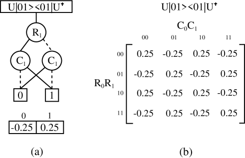
Figure 3: (a) QuIDD for the density matrix resulting from $U|01\rangle\langle 01|U^{\dagger}$, where $U=H\otimes H$, and (b) its explicit matrix form.

Figure 3a shows the QuIDD that results from applying $U$ to an outer product as $U|01\rangle\langle 01|U^{\dagger}$, where $U=H\otimes H$. The $R_{i}$ nodes of the QuIDD encode the binary indices of the rows in the explicit matrix. Similarly, the $C_{i}$ nodes encode the binary indices of the columns. Solid lines leaving a node denote the positive cofactor of the index bit variable (a value of $1$), while dashed lines denote the negative cofactor (a value of $0$). Terminal nodes correspond to the value of the element in the explicit matrix whose binary row/column indices are encoded by the path that was traversed.

Notice that the first and second pairs of rows of the explicit matrix in Fig. 3b are equal, as are the first and second pairs of columns. This redundancy is captured by the QuIDD in Fig. 3a because the QuIDD does not contain any $R_{0}$ or $C_{0}$ nodes. In other words, the values and their locations in the explicit matrix can be completely determined without the superfluous knowledge of the first row and column index bits.

Measurement, matrix multiplication, addition, scalar products, the tensor product, and other operations involving QuIDDs are variations of the well-known $Apply$ algorithm discussed in Sec. 2.2.[22, 21] It has been proven that by interleaving the row and column variables in the variable ordering, QuIDDs can represent and operate on a certain class of matrices and vectors using time and memory resources that are polynomial in the number of qubits. This class includes, but is not limited to, any equal superposition of $n$ qubits, any sequence of $n$ qubits in the computational basis states, $n$-qubit Pauli operators, and $n$-qubit Hadamard operators [21].

Since QuIDDs already have the capability to represent matrices and multiply them [22, 21], extending QuIDDs to encompass the density matrix requires algorithms for the outer product and the partial trace. The outer product involves matrix multiplication between a column vector and its complex-conjugate transpose. Since a column vector QuIDD only depends on row variables, the transpose can be accomplished by swapping the row variables with column variables. The complex conjugate can then be performed with a DFS traversal that replaces terminal node values with their complex conjugates. The original column vector QuIDD is then multiplied by its complex-conjugate transpose using the matrix multiply operation previously defined for QuIDDs [22, 21]. Pseudo-code for this algorithm is given in Fig. 4. Notice that before the result is returned, it is divided by $2^{num\_qubits}$, where $num\_qubits$ is the number of qubits represented by the QuIDD vector. This is done because a QuIDD that only depends on $n$ row variables can be viewed as either a $2^{n}\times 1$ column vector or a $2^{n}\times 2^{n}$ matrix in which all columns are the same. Since matrix multiplication is performed in terms of the latter case [22, 21, 2], the result of the outer product contains values that are multiplied by an extra factor of $2^{n}$, which must be normalized.

$\begin{array}[]{l}\mathbf{Outer\_Product}(Q,num_{q}ubits)\ \{\\ \hskip 10.00002ptQ\_cctrans=\mathbf{Swap\_Row\_Col\_Variables}(Q);\\ \hskip 10.00002ptQ\_cctrans=\mathbf{Complex\_Conj}(Q\_cctrans);\\ \hskip 10.00002ptR=\mathbf{Matrix\_Multiply}(Q,Q\_cctrans);\\ \hskip 10.00002ptR=\mathbf{Scalar\_Div}(Q\_cctrans,2^{num\_qubits});\\ \hskip 10.00002ptreturn\ R;\\ \}\end{array}$

$\begin{array}[]{l}\mathbf{Complex\_Conj}(Q)\ \{\\ \hskip 10.00002ptif\ (\mathbf{Is\_Constant}(Q))\\ \hskip 20.00003ptreturn\ \mathbf{New\_Terminal}({\mathbf{R}eal}(Q),-1*{\mathbf{I}mag}(Q));\\ \hskip 10.00002ptif\ (\mathbf{Table\_Lookup}(computed\_table,Q,R)\\ \hskip 20.00003ptreturnR;\\ \hskip 10.00002ptv=\mathbf{Top\_Var}(Q);\\ \hskip 10.00002ptT=\mathbf{Complex\_Conj}(Q_{v});\\ \hskip 10.00002ptE=\mathbf{Complex\_Conj}(Q_{v^{\prime}});\\ \hskip 10.00002ptR=\mathbf{ITE}(v,T,E);\\ \hskip 10.00002pt\mathbf{Table\_Insert}(computed\_table,Q,R);\\ \hskip 10.00002ptreturn\ R;\\ \}\end{array}$

(a)

(b)

Figure 4: Pseudo-code for (a) the QuIDD outer product and (b) its complex conjugation helper function ${\mathbf{C}omplex\_Conj}$. The code for ${\mathbf{S}calar\_Div}$ is the same as ${\mathbf{C}omplex\_Conj}$, except that in the terminal node case it returns the value of the terminal divided by a scalar. Other functions are typical ADD operations.[2, 18]

To motivate the QuIDD-based partial trace algorithm, we note how the partial trace can be performed with explicit matrices. The trace of a matrix $A$ is the sum of $A$’s diagonal elements. To perform the partial trace over a particular qubit in an $n$-qubit density matrix, the trace operation can be applied iteratively to sub-matrices of the density matrix. Each sub-matrix is composed of four elements with row indices $r0s$ and $r1s$, and column indices $c0d$and $c1d$, where $r$, $s$, $c$, and $d$ are arbitrary sequences of bits which index the $n$-qubit density matrix.

Tracing over these sub-matrices has the effect of reducing the dimensionality of the density matrix by one qubit. A well-known ADD operation which reduces the dimensionality of a matrix is the $Abstract$ operation [2]. Given an arbitrary ADD $f$, abstraction of variable $x_{i}$ eliminates $x_{i}$ from the support of $f$ by combining the positive and negative cofactors of $f$ with respect to $x_{i}$ using some binary operation. In other words, $Abstract(f,x_{i},op)=f_{x_{i}}\ op\ f_{x_{i}^{\prime}}$.

$\begin{array}[]{l}\mathbf{Ptrace}(Q,qubit\_index)\ \{\\ \hskip 10.00002ptif(\mathbf{Is\_Constant}(Q))\\ \hskip 20.00003ptreturn\ Q;\\ \hskip 10.00002pttop\_q=\mathbf{Top\_Var}\hskip 10.00002ptif\ (qubit\_index<\mathbf{Index}(top\_q))\ \{\\ \hskip 20.00003ptR=\mathbf{Apply}(Q,Q,+);\\ \hskip 20.00003ptreturn\ R;\\ \hskip 10.00002pt\}\\ \\ \hskip 10.00002ptif\ (\mathbf{Table\_Lookup}(computed\_table,(Q,qubit\_index),R)\\ \hskip 20.00003ptreturn\ R;\\ \hskip 10.00002ptT=Q_{top\_q};\\ \hskip 10.00002ptE=Q_{top\_q^{\prime}};\\ \\ \hskip 10.00002ptif\ (qubit\_index==\mathbf{Index}(top\_q))\ \{\\ \hskip 20.00003ptif\ (\mathbf{Is\_Constant}(T)\ ||\ \mathbf{Index}(T)>\mathbf{Index}(Q)+1)\\ \hskip 30.00005ptr_{1}=\mathbf{Ptrace}(T,qubit\_index);\\ \hskip 20.00003ptelse\ \{\\ \hskip 30.00005pttop\_T=\mathbf{Top\_Var}(T);\\ \hskip 30.00005ptr_{1}=\mathbf{Ptrace}(T_{top\_T},qubit\_index);\\ \hskip 20.00003pt\}\\ \\ \hskip 20.00003ptif\ (\mathbf{Is\_Constant}(E)\ ||\ \mathbf{Index}(E)>\mathbf{Index}(Q)+1)\\ \hskip 30.00005ptr_{2}=\mathbf{Ptrace}(E,qubit\_index);\\ \hskip 20.00003ptelse\ \{\\ \hskip 30.00005pttop\_E\ \mathbf{Top\_Var}(E);\\ \hskip 30.00005ptr_{2}=\mathbf{Ptrace}(E_{top\_E^{\prime}},qubit\_index);\\ \hskip 20.00003pt\}\\ \hskip 20.00003ptR=\mathbf{Apply}(r_{1},r_{2},+);\\ \hskip 20.00003pt\mathbf{Table\_Insert}(computed\_table,(Q,qubit\_index),R);\\ \hskip 20.00003ptreturn\ R;\\ \hskip 10.00002pt\}\\ \\ \hskip 10.00002ptelse\ \{\hskip 10.00002pt/*\ (qubit\_index>\mathbf{Index}(top\_q)\ */\\ \hskip 20.00003ptr_{1}=\mathbf{Ptrace}(T,qubit\_index);\\ \hskip 20.00003ptr_{2}=\mathbf{Ptrace}(E,qubit\_index);\\ \hskip 20.00003ptR=\mathbf{ITE}(top\_q,r_{1},r_{2});\\ \hskip 20.00003pt\mathbf{Table\_Insert}(computed\_table,(Q,qubit\_index),R);\\ \hskip 20.00003ptreturn\ R;\\ \hskip 10.00002pt\}\\ \}\end{array}$

Figure 5: Pseudo-code for the QuIDD partial trace. The index of the qubit being traced over is $qubit\_index$. Compare this to the pseudo-code for $Abstract()$.[2]

For QuIDDs, there is a one-to-one correspondence between a qubit on wire $i$ (wires are labeled top-down starting at $0$) and variables $R_{i}$ and $C_{i}$. So at first glance, one may suspect that the partial trace of qubit $i$ in $f$ can be achieved by a performing $Abstract(f,R_{i},+)$ followed by $Abstract(f,C_{i},+)$. However, this will add the rows determined by qubit $i$ independently of the columns. The desired behavior is to perform the diagonal addition of sub-matrices by accounting for both the row and column variables due to $i$ simultaneously. The pseudo-code to perform the partial trace correctly is depicted in Fig. 5. In comparing this with the pseudo-code for the $Abstract$ algorithm [2], the main difference is that when $R_{i}$ corresponding to qubit $i$ is reached, we take the positive and negative cofactors twice before making the recursive call. Since the interleaved variable ordering of QuIDDs guarantees that $C_{i}$ immediately follows $R_{i}$ [22, 21], taking the positive and negative cofactors twice simultaneously abstracts both the row and column variables for qubit $i$, achieving the desired result of summing diagonals. In other words, for a QuIDD $f$, the partial trace over qubit $i$ is $Ptrace(f,i)=f_{R_{i}C_{i}}+f_{R_{i}^{\prime}C_{i}^{\prime}}$. Note that in the pseudo-code there are checks for the special case when $C_{i}$ is not in the support of the QuIDD. Not shown in the pseudo-code is book-keeping which shifts up the variables in the resulting QuIDD to fill the hole in the ordering left by the row and column variables that were traced-over.

3.2 QuIDDPro/D

QuIDDPro/D is the implementation of our simulation technique. It was written in C++, and the source code is approximately $17,000$ lines long. The density matrix is represented by a QuIDD class with terminal node values of type $complex<long\ double>$. Gate operators are also represented as QuIDDs. QuIDDPro/D utilizes our earlier QuIDDPro source code [22, 21] and extends it significantly with an implementation of the outer product and partial trace pseudo-code of Fig. 4 and Fig. 5. Additionally, the technique of using an epsilon to deal with precision problems in QuIDDPro [22, 21] has been replaced with a technique that rounds complex numbers to $25$ significant digits. This enhancement allows an end-user to avoid having to find an optimal value of epsilon for a given quantum circuit input. A front-end parser was also created using Flex and Bison to accept a subset of the MATLAB language, which is ideal for describing linear-algebraic operations in a text format. In addition to incorporating a set of well-known numerical functions, the language also supports a number of other functions that are useful in quantum circuit simulation. For example, there is a function for creating controlled-$U$ gates with an arbitrary configuration for the control qubits and user-defined specification of $U$. Functions to perform deterministic measurement, probabilistic measurement, and the partial trace, among others, are also supported. The current version of QuIDDPro/D contains over $65$ functions and language features.

4 EXPERIMENTAL RESULTS

We consider a number of quantum circuit benchmarks which cover errors, error correction, reversible logic, communication, and quantum search. We devised some of the benchmarks, while others are drawn from NIST[4] and from a site devoted to reversible circuits[13]. For every benchmark, the simulation performance of QuIDDPro/D is compared with NIST’s QCSim quantum circuit simulator, which utilizes an explicit array-based computational engine. The results indicate that QuIDDPro/D far outperforms QCSim. All experiments are performed on a 1.2GHz AMD Athlon workstation with 1GB of RAM running Linux.

4.1 Reversible Circuits

Here we examine the performance of QuIDDPro/D simulating a set of reversible circuits, which we define as quantum circuits that perform classical operations.[15] Specifically, if the input qubits of a quantum circuit are all in the computational basis (i.e. they have only $|0\rangle$ or $|1\rangle$ values), there is no quantum noise, and all the gates are NOT variants such as CNOT, Toffoli, X, etc, then the output qubits and all intermediate states will also be in the computational basis. Such a circuit results in a classical logic operation which is reversible in the sense that the inputs can always be derived from the outputs and the circuit function. Reversibility comes from the fact that all quantum operators must be unitary and therefore all have inverses.[15]

The first reversible benchmark we consider is a reversible $4$-bit ripple-carry adder which is depicted in Fig. 6. Since the size of a QuIDD is sensitive to the arrangement of different values of matrix elements, we simulate the adder with varied input values (“rc_adder1” through “rc_adder4”). This is also done for other benchmarks.

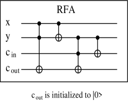
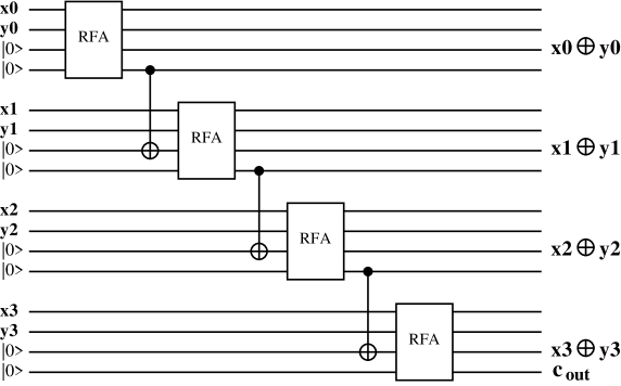
(a)	(b)

Figure 6: (a) An implementation of a reversible full-adder (RFA), and (b) a reversible $4$-bit ripple-carry adder which utilizes the RFA as a module. The reversible ripple-carry adder circuit computes the binary sum of two $4$-bit numbers: $x_{3}x_{2}x_{1}x_{0}\oplus y_{3}y_{2}y_{1}y_{0}$. $c_{out}$ is the final carry bit output from the addition of the most-significant bits ($x_{3}$ and $y_{3}$).

Two other reversible benchmarks we simulate contain fewer qubits but more gates than the ripple-carry adder. One of these benchmarks is a $12$-qubit reversible circuit that outputs a $|1\rangle$ on the last qubit if and only if the number of $|1\rangle$’s in the input qubits is $3$, $4$, $5$, or $6$ (“9sym1” through “9sym5”).[13] The other benchmark is a $15$-qubit reversible circuit that generates the classical Hamming code of the input qubits (“ham15_1” through “ham15_3”).[13]

Performance results for all of these benchmarks are shown in Tab. 1. QuIDDPro/D significantly outperforms QCSim in every case. In fact for circuits of $14$ or more qubits, QCSim requires more than 2GB of memory. Since QCSim uses an explicit array-based engine, it is insensitive to the arrangement and values of elements in matrices. Therefore, one can expect QCSim to use more than 2GB of memory for any benchmark with $14$ or more qubits, regardless of the circuit functionality and input values. Another interesting result is that even though QuIDDPro/D is, in general, sensitive to the arrangement and values of matrix elements, the data indicate that QuIDDPro/D is insensitive to varied inputs on the same circuit for error-free reversible benchmarks. However, QuIDDPro/D still compresses the tremendous amount of redundancy present in these benchmarks, and its performance does vary from one type of circuit to the next.

Table 1: Performance results for QuIDDPro/D and QCSim on the reversible circuit benchmarks. MEM-OUT indicates that a memory usage cutoff of 2GB was exceeded.

Benchmark	No. of	No. of	QuIDDPro/D		QCSim
	Qubits	Gates	Runtime (s)	Peak Memory (MB)	Runtime (s)	Peak Memory (MB)
rc_adder1	16	24	0.44	0.0625	MEM-OUT	MEM-OUT
rc_adder2	16	24	0.44	0.0625	MEM-OUT	MEM-OUT
rc_adder3	16	24	0.44	0.0625	MEM-OUT	MEM-OUT
rc_adder4	16	24	0.44	0.0625	MEM-OUT	MEM-OUT
9sym1	12	29	0.2	0.0586	8.01	128.1
9sym2	12	29	0.2	0.0586	8.02	128.1
9sym3	12	29	0.2	0.0586	8.04	128.1
9sym4	12	29	0.2	0.0586	8	128.1
9sym5	12	29	0.2	0.0586	7.95	128.1
ham15_1	15	148	1.99	0.121	MEM-OUT	MEM-OUT
ham15_2	15	148	2.01	0.121	MEM-OUT	MEM-OUT
ham15_3	15	148	1.99	0.121	MEM-OUT	MEM-OUT

4.2 Error Correction and Communication

Now we analyze the performance of QuIDDPro/D on simulations that incorporate errors and error correction. We consider some simple benchmarks that encode single qubits into Steane’s $7$-qubit error-correcting code[20, 15] and some more complex benchmarks that use the Steane code to correct a combination of bit-flip and phase-flip errors in a half-adder and Grover’s quantum search algorithm.[10] Secure quantum communication is also considered here because eavesdropping disrupts a quantum channel and can be treated as an error.

The first set of benchmarks, “steaneX” and “steaneZ,” each encode a single logical qubit as seven physical qubits with the Steane code and simulate the effect of a probabilistic bit-flip and phase-flip error, respectively.[4] “steaneZ” contains $13$ qubits which are initialized to the mixed state $0.866025|0000000000000\rangle\\ +0.5|0000001000000\rangle$. A combination of gates apply a probabilistic phase-flip on one of the qubits and calculate the error syndrome and error rate. “steaneX” is a $12$ qubit version of the same circuit that simulates a probabilistic bit-flip error.

A more complex benchmark that we simulate is a reversible half-adder with three logical qubits that are encoded into twenty one physical qubits with the Steane code. Additionally, three ancillary qubits are used to track the error rate, giving a total circuit size of twenty four qubits. “hadder1_bf1” through “hadder3_bf3” simulate the half-adder with different numbers of bit-flip errors on various physical qubits in the encoding of one of the logical qubit inputs. Similarly, “hadder1_pf1” through “hadder3_pf3” simulate the half-adder with various phase-flip errors.

Another large benchmark we simulate is an instance of Grover’s quantum search algorithm. Grover’s algorithm searches for a subset of items in an unordered database of $N$ items. Allowed selection criteria are black-box predicates, called oracles, that can be evaluated on any database record. This particular benchmark applies an oracle that searches for one element in a database of four items. It has two logical data qubits and one logical oracle ancillary qubit which are all encoded with the Steane code. Like the half-adder circuit, this results in a total circuit size of twenty four qubits. “grover_s1” simulates the circuit with the encoded qubits in the absence of errors. “grover_s_bf1” and “grover_s_pf1” introduce and correct a bit-flip and phase-flip error, respectively, on one of the physical qubits in the encoding of the logical oracle qubit.

In addition to error modeling and error correction for computational circuits, another important application is secure communication using quantum cryptography. The basic concept is to use a quantum-mechanical phenomenon called entanglement to distribute a shared key. Eavesdropping constitutes a measurement of the quantum state representing the key, disrupting the quantum state. This disruption can be detected by the legitimate communicating parties. Since actual implementations of quantum key distribution have already been demonstrated [19], efficient simulation of these protocols may play a key role in exploring possible improvements. Therefore, we present two benchmarks which implement BB84, one of the earliest quantum key distribution protocols [3]. “bb84Eve” accounts for the case in which an eavesdropper is present (see Fig. 7) and contains $9$ qubits, whereas “bb84NoEve” accounts for the case in which no eavesdropper is present and contains $7$ qubits. In both circuits, all qubits are traced-over at the end except for two qubits reserved to track whether or not the legitimate communicating parties successfully shared a key (BasesEq) and the error due to eavesdropping (Error).

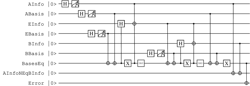
Figure 7: Quantum circuit for the “bb84Eve” benchmark.

Performance results for all of these benchmarks are show in Tab. 2. Again, QuIDDPro/D significantly outperforms QCSim on all benchmarks except for “bb84Eve” and “bb84NoEve.” The performance of QuIDDPro/D and QCSim is about the same for these benchmarks. The reason is that these benchmarks contain fewer qubits than all of the others. Since each additional qubit doubles the size of an explicit density matrix, QCSim has difficulty simulating the larger Steane encoded benchmarks.

Table 2: Performance results for QCSim and QuIDDPro/D on the error-related benchmarks. Runtime results for “bb84NoEve” are below reasonable measurement error. MEM-OUT indicates that a memory usage cutoff of 2GB was exceeded.

Benchmark	No. of	No. of	QuIDDPro/D		QCSim
	Qubits	Gates	Runtime (s)	Peak Memory (MB)	Runtime (s)	Peak Memory (MB)
steaneZ	13	143	0.6	0.672	287	512
steaneX	12	120	0.27	0.68	53.2	128
hadder_bf1	24	49	18.3	1.48	MEM-OUT	MEM-OUT
hadder_bf2	24	49	18.7	1.48	MEM-OUT	MEM-OUT
hadder_bf3	24	49	18.7	1.48	MEM-OUT	MEM-OUT
hadder_pf1	24	51	21.2	1.50	MEM-OUT	MEM-OUT
hadder_pf2	24	51	21.2	1.50	MEM-OUT	MEM-OUT
hadder_pf3	24	51	20.7	1.50	MEM-OUT	MEM-OUT
grover_s1	24	50	2301	94.2	MEM-OUT	MEM-OUT
grover_s_bf1	24	71	2208	94.3	MEM-OUT	MEM-OUT
grover_s_pf1	24	73	2258	94.2	MEM-OUT	MEM-OUT
bb84Eve	9	26	0.02	0.129	0.19	2.0
bb84NoEve	7	14	$<$0.01	0.0313	$<$0.01	0.152

4.3 Scalability and Quantum Search

To test scalability with the number of input qubits, we turn to quantum circuits containing a variable number of input qubits. In particular, we reconsider Grover’s quantum search algorithm. However, for these instances of quantum search, the qubits are not encoded with the Steane code, and errors are not introduced. The oracle performs the same function as the one described in the last subsection except that the number of data qubits ranges from five to twenty.

Performance results for these circuit benchmarks are shown in Tab. 3. Again, QuIDDPro/D has significantly better performance. These results highlight the fact that QCSim’s explicit representation of the density matrix becomes an asymptotic bottleneck as $n$ increases, whereas QuIDDPro/D’s compression of the density matrix and operators scales extremely well.

Table 3: Performance results for QCSim and QuIDDPro/D on the Grover’s quantum search benchmark. MEM-OUT indicates that a memory usage cutoff of 2GB was exceeded.

No. of	No. of	QuIDDPro/D		QCSim
Qubits	Gates	Runtime (s)	Peak Memory (MB)	Runtime (s)	Peak Memory (MB)
5	32	0.05	0.0234	0.01	0.00781
6	50	0.07	0.0391	0.01	0.0352
7	84	0.11	0.043	0.08	0.152
8	126	0.16	0.0586	0.54	0.625
9	208	0.27	0.0742	3.64	2.50
10	324	0.42	0.0742	23.2	10.0
11	520	0.66	0.0898	151	40.0
12	792	1.03	0.105	933	160
13	1224	1.52	0.141	5900	640
14	1872	2.41	0.125	MEM-OUT	MEM-OUT
15	2828	3.62	0.129	MEM-OUT	MEM-OUT
16	4290	5.55	0.145	MEM-OUT	MEM-OUT
17	6464	8.29	0.152	MEM-OUT	MEM-OUT
18	9690	12.7	0.246	MEM-OUT	MEM-OUT
19	14508	18.8	0.199	MEM-OUT	MEM-OUT
20	21622	28.9	0.203	MEM-OUT	MEM-OUT

5 CONCLUSIONS AND FUTURE WORK

We have described a new graph-based simulation technique that enables efficient density matrix simulation of quantum circuits. We implemented this technique in the QuIDDPro/D simulator. QuIDDPro/D uses the QuIDD data structure to compress redundancy in the gate operators and the density matrix. As a result, the time and memory complexity of QuIDDPro/D varies depending on the structure of the circuit. However, we demonstrated that QuIDDPro/D exhibited superior performance on a set of benchmarks which incorporate qubit errors, mixed states, error correction, quantum communication, and quantum search. This result indicates that there is a great deal of structure in practical quantum circuits that graph-based algorithms like those implemented in QuIDDPro/D exploit.

We are currently seeking to further improve quantum circuit simulation. For example, algorithmic improvements directed at specific gates could enhance an existing simulator’s performance. With regard to QuIDDPro/D in particular, we are also exploring the possibility of using “read-k” ADDs and edge-valued diagrams (EVDDs) in an attempt to elicit more compression. Lastly, we are studying technology-specific circuits for quantum-information processing. Optionally incorporating technology-specific details may lead to simulation results that are more meaningful to physicists building real devices, particularly with regard to error modeling.