Quantum cryptography with correlated twin laser beams

Abstract

The data transmission protocol, based on the use of a strongly correlated pair of laser beams, is proposed. The properties of the corresponding states are described in detail. The protocol is based on the strong correlation of photon numbers in both beams in each measurement. The protocol stability against the interception attempts is analyzed.

1 Introduction.

The main goal of the quantum cryptography, which is the part of the quantum computing, is in development of the reliable and secure procedures of generation and transmission of a cryptographic key, which can be used for the encryption of the further communication. In the last years, some progress was achieved in this area [1, 2, 3] and protocols were developed on the basis of the quantum entanglement [5, 6] of weak beams and the sigle [7, 8, 21] or four photon states [9], mostly by means of adjusting and detecting their polarization angles [11].

Those methods were realized experimentally [6, 10], but still they are difficult for implementation in particular because of the complexity of a few photon state preparation and detection. If a bit is transferred by a one or a few photons, the detection of each state requires numerous acts of measurements, this slows down the information flow. This relates even to the most successful realizations [19, 20] and that’s why the new ideas are still in need.

In this work we propose and examine the cryptographic method based on the use of a correlated two-mode laser beam for a secure key generation and transmission between two sites. Such and similar beams are actively experimentally studied last time [12, 13, 14]. Therefore we examine in detail the properties of the states, which describe the two-mode correlated laser beams, investigate the dependence of these properties on the beam intensity, and analyze the possibility to use such beams in the data channels. Also we study the question of stability of such channels against the elementary eavesdropping attacks.

2 The coherently correlated state

The two-mode coherently correlated state is the way we refer to the generalized coherent state in the meaning by Perelomov [4]. Such states were studied by Arvind [15] and others [16, 17, 18] as the pair-coherent states.

The two-mode coherently correlated state can be described by its presentation through series by Fock states:

$$\left|\lambda\right\rangle=\frac{1}{\sqrt{I_{0}\left(2\left|\lambda\right|\right)}}\sum{\frac{\lambda^{n}}{n!}\left|{nn}\right\rangle}$$ (1)

Here we use the designation $\left|{nn}\right\rangle=\left|n\right\rangle_{1}\otimes\left|n\right\rangle_{2}$, where $\left|n\right\rangle_{1}$ and $\left|n\right\rangle_{2}$stand for the states of the $1^{st}$ and $2^{nd}$ modes accordingly, represented by their photon numbers. The states (1) are not the eigenstates for each of the operators separately, but are the eigenstates for the product of annihilation operators:

$$a_{1}a_{2}\left|\lambda\right\rangle=\lambda\left|\lambda\right\rangle.$$ (2)

Such states can also be obtained from the zero state:

$$\left|\lambda\right\rangle=\frac{1}{\sqrt{I_{0}\left(2\left|\lambda\right|\right)}}I_{0}(\lambda a_{1}^{+}a_{2}^{+})\left|0\right\rangle$$ (3)

Hereinafter we denote the two-mode coherently correlated states as the TMCC states. In this work we assume that two laser beams, which are propagating independently from each other, correspond to the two modes of the TMCC state. States of beams are mutually correlated. (Surely, the TMCC state can also be represented in another way, for example, as a beam consisting of two correlated polarizations)

An observable of such a pair of beams (for example, the vector-potential) is given by the expression:

$$A=\varphi_{1}^{\ast}(x,t)a_{1}^{+}+\varphi_{1}(x,t)a_{1}+\varphi_{2}^{\ast}(x,t)a_{2}^{+}+\varphi_{2}(x,t)a_{2}$$ (4)

This expression has explicit spatial dependence $\varphi(x,t)$ and the quantum operators $a,a^{+}$.

Let’s compare the TMCC state to the usual, noncorrelated two-mode coherent state $|\alpha\rangle=|\alpha_{1}\rangle_{1}\otimes|\alpha_{2}\rangle_{2}$. Each of the two modes of such state is given by an expression:

$$\left|{\alpha_{i}}\right\rangle=e^{-\frac{\left|\alpha\right|^{2}}{2}}\sum{\frac{\alpha_{i}^{n}}{\sqrt{n!}}\left|n\right\rangle},i=1,2$$ (5)

Such states are the eigenstates for the corresponding annihilation operators: $a_{i}\left|{\alpha_{i}}\right\rangle=\alpha_{i}\left|{\alpha_{i}}\right\rangle$

Thus the mean value of the vector-potential (4) is

$$\left\langle A\right\rangle=\varphi_{1}\alpha_{1}+\varphi_{1}^{\ast}\alpha_{1}^{\ast}+\varphi_{2}\alpha_{2}+\varphi_{2}^{\ast}\alpha_{2}^{\ast}$$ (6)

and this is the show of the quasiclassical properties of the beam (5).

In the case of the TMCC state the mean value of any characteristic, which is linear in field, turns to be equal to 0, because during the averaging by the 1^st mode the $a_{1}$ converts $\left|{n,n}\right\rangle$ to $\left|{n-1,n}\right\rangle$, which is orthogonal to all the present state terms, so $\left\langle{\lambda_{i}}\right|a_{i}\left|{\lambda_{i}}\right\rangle=0$, that’s why

$$\left\langle A\right\rangle=\left\langle\lambda\right|A\left|\lambda\right\rangle=\left\{\begin{array}[]{l}\varphi_{1}^{\ast}(x,t)\left\langle\lambda\right|a_{1}^{+}\left|\lambda\right\rangle+\varphi_{1}(x,t)\left\langle\lambda\right|a_{1}\left|\lambda\right\rangle+\\ \varphi_{2}^{\ast}(x,t)\left\langle\lambda\right|a_{2}^{+}\left|\lambda\right\rangle+\varphi_{2}(x,t)\left\langle\lambda\right|a_{2}\left|\lambda\right\rangle\end{array}\right.=0$$ (7)

and so the quasiclassical properties in their usual meaning are absent in this case. But they become apparent in the spatial correlation function

$$\gamma(x,t;{x}^{\prime},{t}^{\prime})=\left\{\begin{array}[]{l}\left\langle{A(x,t)\cdot A({x}^{\prime},{t}^{\prime})}\right\rangle-\left\langle{A(x,t)}\right\rangle\cdot\left\langle{A({x}^{\prime},{t}^{\prime})}\right\rangle\\ =\left\langle{A(x,t)\cdot A({x}^{\prime},{t}^{\prime})}\right\rangle\end{array}\right.,$$ (8)

which is non-zero because $\left\langle{A(x,t)\cdot A({x}^{\prime},{t}^{\prime})}\right\rangle$ contains mean values for the products of quantum operators and some of them are non-zero.

$$\left\langle{A\left(x,t\right)\cdot A\left(x^{\prime},t^{\prime}\right)}\right\rangle={\left\{\begin{array}[]{l}\varphi_{1}^{\ast}\left(x,t\right)\varphi_{1}\left(x^{\prime},t^{\prime}\right)\left\langle\lambda\right|\hat{a}_{1}^{+}\hat{a}_{1}\left|\lambda\right\rangle+\\ \varphi_{1}^{\ast}\left(x,t\right)\varphi_{2}^{\ast}\left(x^{\prime},t^{\prime}\right)\left\langle\lambda\right|\hat{a}_{1}^{+}\hat{a}_{2}^{+}\left|\lambda\right\rangle+\\ \varphi_{1}\left(x,t\right)\varphi_{1}^{\ast}\left(x^{\prime},t^{\prime}\right)\left\langle\lambda\right|\hat{a}_{1}\hat{a}_{1}^{+}\left|\lambda\right\rangle+\\ \varphi_{1}\left(x,t\right)\varphi_{2}\left(x^{\prime},t^{\prime}\right)\left\langle\lambda\right|\hat{a}_{1}\hat{a}_{2}\left|\lambda\right\rangle+\\ \varphi_{2}^{\ast}\left(x,t\right)\varphi_{1}^{\ast}\left(x^{\prime},t^{\prime}\right)\left\langle\lambda\right|\hat{a}_{2}^{+}\hat{a}_{1}^{+}\left|\lambda\right\rangle+\\ \varphi_{2}^{\ast}\left(x,t\right)\varphi_{2}\left(x^{\prime},t^{\prime}\right)\left\langle\lambda\right|\hat{a}_{2}^{+}\hat{a}_{2}\left|\lambda\right\rangle+\\ \varphi_{2}\left(x,t\right)\varphi_{1}\left(x^{\prime},t^{\prime}\right)\left\langle\lambda\right|\hat{a}_{2}\hat{a}_{1}\left|\lambda\right\rangle+\\ \varphi_{2}\left(x,t\right)\varphi_{2}^{\ast}\left(x^{\prime},t^{\prime}\right)\left\langle\lambda\right|\hat{a}_{2}\hat{a}_{2}^{+}\left|\lambda\right\rangle\end{array}\right.}$$ (9)

3 Communication via quantum channel

Let we have to establish a secure quantum channel between two parties (Figure 1). Alice has the laser on her side, which produces two beams in the TMCC state. The optical channel is organized in such a way, that Alice receives one of the modes, the first, for example, i.e. $\varphi_{A}\equiv\varphi_{1}$,$\varphi_{A}(x_{A},t_{0})=1$ , and Bob receives another one, i.e. $\varphi_{B}\equiv\varphi_{2}$ ,$\varphi_{B}(x_{B},t_{0})=1$ at any moment of measurement $t_{0}$, where $x_{A}$and $x_{B}$are Alice’s and Bob’s locations respectively. Accordingly, Alice cannot measure the Bob’s beam and vice versa:$\varphi_{B}(x_{A},t_{0})=0$, $\varphi_{A}(x_{B},t_{0})=0$. At that the field is:

$$A=\varphi_{A}^{\ast}(x,t)a_{A}^{+}+\varphi_{A}(x,t)a_{A}+\varphi_{B}^{\ast}(x,t)a_{B}^{+}+\varphi_{B}(x,t)a_{B}$$ (10)

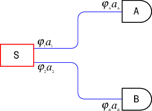
Figure 1: Quantum channel between two parties with a TMCC source

The intensity of the radiation, registered by Alice is proportional to the mean of the $N_{A}=a_{A}^{+}a_{A}$ operator, which is the number of the photons in the $1^{st}$ mode and it is similarly for Bob with $N_{B}=a_{B}^{+}a_{B}$ . Thus the mean observable values, which characterize the results of the measurements, taken by Alice and Bob, are

$$\left\langle{N_{A,B}}\right\rangle=\left\langle\lambda\right|a_{A,B}^{+}a_{A,B}\left|\lambda\right\rangle=\frac{\left|\lambda^{2}\right|I_{1}\left({2\left|\lambda\right|}\right)}{I_{0}\left({2\left|\lambda\right|}\right)}$$ (11)

These values are squared in field, and thus their mean values don’t turn to zero.

$$\left\langle{N_{A,B}^{2}}\right\rangle=\left\langle{N_{A}N_{B}}\right\rangle=\left\langle\lambda\right|a_{A}^{+}a_{A}a_{B}^{+}a_{B}\left|\lambda\right\rangle=\left|\lambda\right|^{2}$$ (12)

The measurements have the statistical uncertainty, caused by quantum fluctuations. For each of the observers the uncertainty can be characterized by the corresponding dispersion:

$$\sigma_{A,B}^{2}=\left\langle{N_{A,B}^{2}}\right\rangle-\left\langle{N_{A,B}}\right\rangle^{2}$$ (13)

Taking into account (12), we get the following expression:

$$\sigma_{A,B}^{2}=\left|\lambda\right|^{2}\left({1-\left({\frac{I_{1}\left({2\left|\lambda\right|}\right)}{I_{0}\left({2\left|\lambda\right|}\right)}}\right)^{2}}\right)$$ (14)

The interdependence of the results of measurements taken by Alice and Bob can by characterized by the correlation function:

$$g_{AB}=<N_{A}N_{B}>-<N_{A}><N_{B}>$$ (15)

It’s useful to describe the channel quality by the relative correlation, which is

$$\rho_{AB}=\frac{<N_{A}N_{B}>-<N_{A}><N_{B}>}{\sigma_{A}\sigma_{B}}$$ (16)

The main feature of the TMCC state is that the value $\rho_{AB}$ is exactly equal to 1, while in the case of non-correlated beams we would get $\rho_{AB}=0$. This means that the measurements of the photon numbers, got by Alice and Bob, each with her/his own detector, not only show the same mean values, but even have the same deflection from the mean values.

The laser beam is the semi-classical radiation with well defined phase, but due to the uncertainty principle for the number of photons and the phase of the radiation, there is a large enough uncertainty in the photon numbers, this can be seen from the dispersion expression (14). Thus one can observe the noise, which is similar to the shot noise in an electron tube. In the TMCC radiation the characteristics of such noise for each of the modes are amazingly well correlated to each other. This fact enables the use of such radiation for generation of a random code, which will be equally good received by two mutually remote detectors.

4 The protocol

We propose the following scheme for the TMCC-based protocol. The laser is set up to produce the constant mean number of photons during the session and both parties know this number. At some moment Alice and Bob start the measurements. They detect the number of photons at unit time by measuring the integrated intensity of the corresponding incoming beam. If the number of photons for the specific unit time is larger than the known expected mean (which is due to the shot noise), the next bit of the generated code is considered to have the value “1”. If the measured number is less than the expected mean, the next bit is considered to be equal to “0”. The procedure is repeated until both, Alice and Bob, get enough bits for the cryptographic key. The described protocol can be supplied with the procedures of the cryptographic control.

5 Eavesdropping

Since the proposed protocol uses the scheme, which differs from the well-known schemes, based on the entangled states of weak beams, it’s useful to study it’s stability against the listening-in. We don’t cover all possible eavesdropping attacks here, taking into consideration only the basic listening-in as the preliminary demonstration of the TMCC-channel security and protectability.

Let’s assume that some eavesdropping intruder (her name is Eve) tries to get the key being transferred between Alice and Bob through the quantum channel. In order to do this, Eve has to split and avert a part of the beam, which goes to Bob and detect its intensity by installing a detector at her side (figure 2). The field amplitude of the beam splits then in some $p:q$ ratio and thus instead of the quantum mode we have to use the superposition

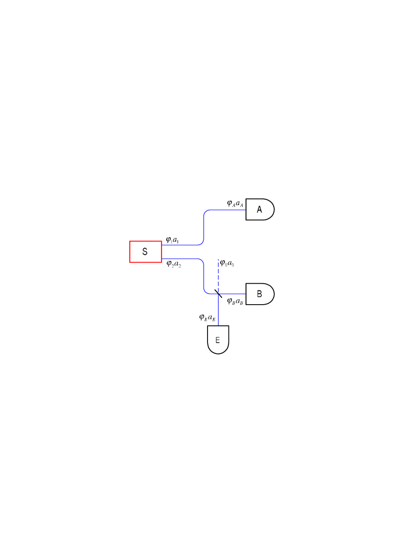
Figure 2: Eavesdropping attack on a TMCC-based quantum channel

$$A=\varphi_{A}^{\ast}(x,t)a_{A}^{+}+\varphi_{A}(x,t)a_{A}+\varphi_{B}(x,t)a_{B}+\varphi_{B}^{\ast}(x,t)a_{B}^{+}+$$

$$+\varphi_{E}(x,t)a_{E}+\varphi_{E}^{\ast}(x,t)a_{E}^{+}$$ (17)

Obviously, $\varphi_{B}(x_{B},t_{0})=1$,$\varphi_{E}(x_{E},t_{0})=1$ and $\varphi_{E}(x_{B},t_{0})=0$, $\varphi_{B}(x_{E},t_{0})=0$, $\varphi_{A}(x_{E},t_{0})=0$. The 2^nd mode is decomposed on the basis, which consists of the modes coming to Bob and Eve. In order to describe the properties of this beam, we add a mode to the basis of Bob and Eve, which is orthogonal to $\varphi_{2}$:

$$\varphi_{0}=-q\varphi_{B}+p\varphi_{E}$$ (18)

Without the eavesdropping (and, thus, without the splitter), Eve receives only the $\varphi_{0}$ mode, in which the laser doesn’t radiate, i.e. $\varphi_{0}=\varphi_{E}$ and $\varphi_{2}=\varphi_{B}$.

The following conversion of operators corresponds to this decomposition:

$$a_{2}=pa_{B}+qa_{E},$$ (19)

$$a_{0}=-qa_{B}+pa_{E}$$ (20)

Thus

$$\varphi_{0}a_{0}+\varphi_{2}a_{2}=\varphi_{B}a_{B}+\varphi_{E}a_{E},$$ (21)

and similarly for the hermitian-conjugate operators.

These transformations change the state (3) to:

$$\left|\lambda\right\rangle=\frac{1}{\sqrt{I_{0}\left(2\left|\lambda\right|\right)}}I_{0}(\lambda a_{A}^{+}(pa_{B}^{+}+qa_{E}^{+})\left|0\right\rangle$$ (22)

Mean observable values in this case are

$$\left\langle{N_{A}}\right\rangle=\left\langle\lambda\right|a_{A}^{+}a_{A}\left|\lambda\right\rangle=\frac{\left|\lambda\right|^{2}I_{1}\left({2\left|\lambda\right|}\right)}{I_{0}\left({2\left|\lambda\right|}\right)},$$ (23)

$$\left\langle{N_{B}}\right\rangle=\left\langle\lambda\right|a_{B}^{+}a_{B}\left|\lambda\right\rangle=p^{2}\frac{\left|\lambda\right|^{2}I_{1}\left({2\left|\lambda\right|}\right)}{I_{0}\left({2\left|\lambda\right|}\right)},$$ (24)

$$\left\langle{N_{E}}\right\rangle=\left\langle\lambda\right|a_{E}^{+}a_{E}\left|\lambda\right\rangle=(1-p^{2})\frac{\left|\lambda\right|^{2}I_{1}\left({2\left|\lambda\right|}\right)}{I_{0}\left({2\left|\lambda\right|}\right)},$$ (25)

Besides we must take into account the mean values of combinations of these operators:

$$\left\langle{N_{A}N_{B}}\right\rangle=\left\langle\lambda\right|a_{A}^{+}a_{A}a_{B}^{+}a_{B}\left|\lambda\right\rangle=p^{2}\left|\lambda\right|^{2}$$ (26)

$$\left\langle{N_{A}N_{E}}\right\rangle=\left\langle\lambda\right|a_{A}^{+}a_{A}a_{E}^{+}a_{E}\left|\lambda\right\rangle=(1-p^{2})\left|\lambda\right|^{2}$$ (27)

and

$$\left\langle{N_{A}^{2}}\right\rangle=\left\langle\lambda\right|a_{A}^{+}a_{A}a_{A}^{+}a_{A}\left|\lambda\right\rangle=\left|\lambda\right|^{2}$$ (28)

$$\left\langle{N_{B}^{2}}\right\rangle=\left\langle\lambda\right|a_{B}^{+}a_{B}a_{B}^{+}a_{B}\left|\lambda\right\rangle=p^{4}\left|\lambda\right|^{2}+p^{2}(1-p^{2})\frac{\left|\lambda\right|^{2}I_{1}\left({2\left|\lambda\right|}\right)}{I_{0}\left({2\left|\lambda\right|}\right)}$$ (29)

$$\left\langle{N_{E}^{2}}\right\rangle=\left\langle\lambda\right|a_{E}^{+}a_{E}a_{E}^{+}a_{E}\left|\lambda\right\rangle=(1-p^{2})^{2}\left|\lambda\right|^{2}+p^{2}(1-p^{2})\frac{\left|\lambda\right|^{2}I_{1}\left({2\left|\lambda\right|}\right)}{I_{0}\left({2\left|\lambda\right|}\right)}$$ (30)

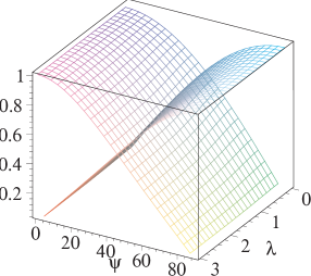
Figure 3: Absolute Alice-Bob and Alice-Eve correlation dependence on the intensity of beam $\lambda$ and the extent of eavesdropping expressed as $p=cos\psi$ for the normalization $p^{2}+q^{2}=1$

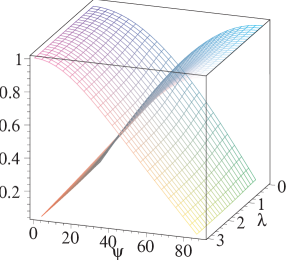
Figure 4: Relative Alice-Bob and Alice-Eve correlation dependence on the intensity of beam $\lambda$ and the extent $p=cos\psi$ of eavesdropping

With these values we can estimate how the Alice-Bob and Alice-Eve correlations depend on the activity of an eavesdropper, which is characterized by the parameter $p$ and on the intensity of the beam. The graphs for these dependencies are given for both, absolute and relative, correlations in figure 3 and figure 4 respectively. One can see that in the case of the weak intercept the results of the Bob’s measurements almost do not change, but at that, if the mean number of photon for Eve in less than 1, she can’t really distinguish between the 0 bit value and 1, thus the eavesdropping isn’t effective. If it becomes effective, Bob experiences the same loses in the transmission quality, the Alice-Bob correlation becomes significantly less than 1 and the channel gets destroyed. This is caused by the fact that each photon, intercepted by Eve gets absorbed on her detector and thus can’t be received by Bob.

6 Conclusions

Correlated coherent states of the two-mode laser beam (TMCC states) show interesting properties, which can be used, in particular, for the tasks of the quantum communication and cryptography.

On the one hand, each of the modes looks like a flow of the independent photons rather then a coherent beam, since mean values of the operators, which are linear in field, are equal to 0 for each mode separately.

On the other hand, the strong correlation between the results of measurements for each of the modes takes place. This correlation shows itself in the fact that in each of the modes numbers of photons are the same and even the shot noise shows itself equally in the both modes. This enables the use of the TMCC state as the generator and carrier of random keys. At that, any signficiant attempt of the information intercept in any of the channels sharply reduces the correlation, leading to the destruction of the channel and, as a consequence, to detection of an eavesdropping. Thus, the TMCC-laser generates and transmits exactly the 2 copies of a random key. Unlike the single or two-photon schemes, which require large numbers of transmission reiterations to obtain the statistically significant results, the TMCC beam can be intensive enough to make each single measurement statistically significant and thus to use single impulse for each piece of information, and remain cryptographically steady. This allows to essentially increase the effective data transfer rate and distance.

References

References

• [1] Nicolas Gisin, Gregoire Ribordy, Wolfgang Tittel, Hugo Zbinden. Quantum Cryptography. Preprint: quant-ph/0101098
• [2] Matthias Christandl, Renato Renner, Artur Ekert. A Generic Security Proof for Quantum Key Distribution. Preprint: quant-ph/0402131
• [3] Nicolas Gisin, Nicolas Brunner. Quantum cryptography with and without entanglement. Preprint: quant-ph/0312011
• [4] A. Perelomov, Generalized Coherent States and Their Applications (Springer, Berlin, 1986).
• [5] Wolfgang Tittel, Gregor Weihs. Photonic Entanglement for Fundamental Tests and Quantum Communication. quant-ph/0107156
• [6] A. Ekert, Phys. Rev. Lett. 67, 661 (1991) entprotexp D. S. Naik et al., Phys. Rev. Lett. 84, 4732 (2000)
• [7] C. H. Bennett, Phys. Rev. Lett. 68, 3121 (1992)
• [8] C. K. Hong and L. Mandel, Phys. Rev. Lett. 56, 58 (1986)
• [9] C. H. Bennett and G. Brassard , Quantum cryptography: public key distribution and coin tossing , Int . conf. Comput ers, Syst ems & Signal Processing, Bangalore, India, 1984, 175- 179.
• [10] T. Jennewein et al., Phys. Rev. Lett. 84, 4729 (2000)
• [11] A.C. Funk, M.G. Raymer. Quantum key distribution using non-classical photon number correlations in macroscopic light pulses. quant-ph/0109071
• [12] Yun Zhang, Katsuyuki Kasai, Kazuhiro Hayasaka. Quantum channel using photon number correlated twin beams. quant-ph/0401033, Optics, Express 11, 3592 (2003)
• [13] L. A. Wu, H. J. Kimble, J. L. Hall, and H. F. Wu, Generation of squeezed states by parametric down conversion, Phys. Rev. Lett. 57, 2520-2524 (1986).
• [14] H. Wang, Y. Zhang, Q. Pan, H. Su, A. Porzio, C. D. Xie, and K. C. Peng, Experimental realization of a quantum measurement for intensity difference fluctuation using a beam splitter, Phys. Rev. Lett. 82, 1414-1417 (1999).
• [15] Arvind, N. Mukunda and R. Simon, Characterisations of Classical and Non-classical states of Quantised Radiation. quant-ph/9512020.
• [16] D. Bhaumik, K. Bhaumik, and B. Dutta-Roy J. Phys. A 9, 1507 (1976);
• [17] G. S. Agarwal, Phys. Rev. Letters 57, 827 (1986);
• [18] G. S. Agarwal, JOSA B 5, 1940 (1988).
• [19] F. Grosshans at al. Nature 421, 238-241 (2003).
• [20] F. Grosshans and Ph. Grangier, Phys. Rev. Lett. 88, 057902 (2002).
• [21] R. Alleaume at al. Experimental open air quantum key distribution with a single photon source. quant-ph/0402110.