Upper bounds on success probabilities in linear optics

Abstract

We develop an abstract way of defining linear-optics networks designed to perform quantum information tasks such as quantum gates. We will be mainly concerned with the nonlinear sign shift gate, but it will become obvious that all other gates can be treated in a similar manner. The abstract scheme is extremely well suited for analytical as well as numerical investigations since it reduces the number of parameters for a general setting. With that we show numerically and partially analytically for a wide class of states that the success probability of generating a nonlinear sign shift gate does not exceed $1/4$ which to our knowledge is the strongest bound to date.

I Introduction

One of the possible physical realisations of quantum information processing is to use conditional measurements in an all-optical passive interferometric scheme. Within this framework, there are many possibilities to encode qubits. Important examples are encodings in superposition states of one photonic excitation in two modes KLM , in the polarization state of a photon Koashi01 ; Pittman , or in the occupation number states of one mode. In this paper, we will follow the latter approach. Hence, we will denote by $|0\rangle$, $|1\rangle$ etc. the vacuum state, the single-photon Fock state and so on. A crucial part of building elementary quantum gates with this encoding is the ability to perform a desired operation on two single photons simultaneously. As an example, the controlled-$\sigma_{z}$ operation amounts to changing the sign of the two-mode state $|11\rangle$ to $-|11\rangle$ thereby leaving the other three basis states $|00\rangle$, $|01\rangle$ and $|10\rangle$ untouched. The unitary operator associated with this quantum gate can be written in the form $e^{i\pi\hat{n}_{1}\hat{n}_{2}}$ where the $\hat{n}_{i}$ are the number operators of the photons in mode $i$. This unitary evolution operator is quartic in the photonic amplitude operators and obviously stems from a nonlinear interaction Hamiltonian with (scaled) ‘strength’ $\pi$. Apparently, neither fourth-order quantum electrodynamics nor materials with effective Kerr nonlinearities reach the order of magnitude required to perform the operation.

There is, however, an elegant way to circumvent the problem of deterministically generating the nonlinear evolution. The idea is borrowed from the well-known theory of quantum-state engineering (cf. Ref. Welsch and references cited therein) where two optical fields in known quantum states are mixed at a beam splitter and postselection is performed subject to a specific measurement outcome in the process of photo-detection in one output arm. This idea has been generalised in KLM ; Koashi01 to unknown quantum states in one input arm of the beam splitter (which results in what one may call quantum-gate engineering). The conditioning on a certain photo-detection event has two consequences: (i) the effective generation of a nonlinear interaction Hamiltonian via postselection, and (ii) the probabilistic nature of the process due to the selection of a subset of all possible measurement outcomes. We can equivalently call this procedure the generation of measurement-induced nonlinearities Scheel03 .

The particular example which has been elaborated in KLM is the nonlinear sign shift (NSS) gate which is described by the transformation

$$c_{0}|0\rangle+c_{1}|1\rangle+c_{2}|2\rangle\mapsto c_{0}|0\rangle+c_{1}|1\rangle-c_{2}|2\rangle\,.$$ (1)

This NSS gate is intimately connected to the above-mentioned controlled-$\sigma_{z}$ operation when noting that two NSS gates in each arm of a balanced Mach–Zehnder interferometer is equivalent to a single controlled-$\sigma_{z}$ gate (Fig. 1).

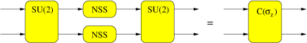
Figure 1: Two nonlinear sign shift (NSS) gates inside a balanced Mach–Zehnder interferometer are equivalent to a two-mode controlled-$\sigma_{z}$ gate. Beam splitters are denoted by their group action as SU($2$).

Several different conditional measurement schemes have been found that generate a NSS KLM ; Scheel03 ; Ralph01 . In all cases, the maximal success probability was found to be $1/4$. The question that arises in this context is: what is the reason for this particular value and is there a general upper limit on the achievable success probability? For the special case of a beam splitter network with ancilla modes containing at most one photon each, it has been shown analytically that the probability is bounded from above by $1/2$ Knill03 . This bound is not necessarily tight since it allows even for conditional dynamics, i.e. post-processing depending on the outcome of a measurement. Note also that even then the success probability does not reach unity.

In this article we introduce a compact model for general linear optics networks. What we will show with this model is that in broad classes of conditional networks, the success probability will not exceed the value of $1/4$ regardless of the dimensionality of the ancilla state used. Although we do not have a fully analytical proof for this claim, we will provide strong numerical evidence and show steps towards a final proof.

This paper is organised as follows. In Sec. II we will describe the abstract conditional measurement scheme we will investigate. This scheme is particularly simple but includes all known networks so far. In section III the evaluation of the success probability in the general case is prepared. The theory of a general two-dimensional ancilla state is presented in Sec. IV followed by a discussion of special cases of three-dimensional ancillas in Sec. V. In the last part, we will give an outlook into possible future work in that direction.

II A general conditional measurement scheme

In this section we will describe an abstract conditional measurement scheme that will allow us to investigate the success probabilities of conditional optical networks without going into the detail of the specific network. Throughout this article we will focus solely onto the NSS gate, noting that other nonlinear gates can be treated analogously. With single-photon sources and single-photon detectors it is known that the NSS gate can be realised by the beam splitter network shown in Fig. 2 Scheel03 .

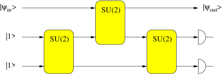
Figure 2: Beam splitter network realising the nonlinear sign shift.

This network represents a group element of the unitary group SU($3$) (note that a single lossless beam splitter acts as an element of SU($2$) on the photonic amplitude operators beamsplitter ).

It was noted some years ago that any U($N$) group element can be realised by a triangle-shaped beam splitter network Reck94 . Therefore, in order to generalise the network in Fig. 2 to incorporate an arbitrary number of ancilla modes in arbitrary initial states, we note that only a single beam splitter actually connects the ancilla state(s) to the signal mode we want to act upon. This means that there are several beam splitters that actually prepare a certain ancilla state, feed them into this single ‘active’ beam splitter which is then followed by another set of beam splitters that prepare the ancilla state for the detection process. Hence, we can schematically represent the whole network by three blocks – the preparation ‘P’ of the ancilla state from some given product states, the single ‘active’ beam splitter ‘A’ connecting signal and ancilla modes, and the detection stage ‘D’ in which the ancilla, for some given initial states, is again decomposed into product states (see Fig. 3).

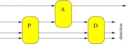
Figure 3: Preparation stage ‘P’ of the ancilla state that is fed into the ‘active’ beam splitter ‘A’, and decomposition stage ‘D’ for detection.

This will be the general conditional measurement scheme we will be looking at.

We can even go one step further by not requiring the preparation and detection stages ‘P’ and ‘D’ to be realised by linear optical elements. Instead, we will try to answer the question of upper bounds for the success probability without this requirement. For that purpose, we divide the total ancilla state into one mode that impinges onto the ‘active’ beam splitter ‘A’ and mixes with the signal mode, and the remaining modes.

From the general theory of measurement-induced nonlinearities we know that, in order to realise an NSS gate, we need to generate an operator which is a polynomial in the number operator Scheel03 . The reasons for this constraint are on one hand the requirement to produce an output state in a Hilbert space that is isomorphic to the Hilbert space of the input state, and on the other hand the necessity to be able to operate on each basis state individually. We can rephrase these conditions, made from an operator point of view, as a requirement on the ancilla state. Isomorphism between the two Hilbert spaces of input and output signal modes can only be achieved if the ancilla is restricted to a state with fixed photon number and if the number of detected photons equals the number of photons in the ancilla. In what follows, we will therefore restrict our attention to ancilla states with fixed photon numbers and the detection of the same number of photons without losing generality.

From these observation it follows that it suffices to consider ancilla state containing exactly $N$ photons, which can hence be written in the form

$$\sum\limits_{k=0}^{N}\gamma_{k}|k\rangle|A_{N-k}\rangle\,,$$ (2)

where $|k\rangle$ is the $k$-photon Fock state impinging on ‘A’. On the other hand, the state $|A_{N-k}\rangle$ can be any multi-mode state as long as it contains exactly $N-k$ photons. This means that we impose no restriction on the number of ancilla modes. Neither have we said anything about the possibility of creating this state with linear optical elements from suitable product states, which is a question that can be addressed separately. The $\gamma_{k}$ can be chosen to be real, since any phase can be absorbed into the definition of $|A_{N-k}\rangle$, and then fulfil the normalisation condition $\sum_{k}\gamma_{k}^{2}=1$. The tensor-product state impinging onto ‘A’ is thus

$$\Big{(}c_{0}|0\rangle+c_{1}|1\rangle+c_{2}|2\rangle\Big{)}\otimes\sum\limits_{k=0}^{N}\gamma_{k}|k\rangle|A_{N-k}\rangle\,.$$ (3)

So far, we have not said anything about the detection process itself, we only select the contributions containing exactly $N$ photons. That leaves us with a transformed state

$$c_{0}|0\rangle\sum\limits_{k=0}^{N}\gamma_{k}|k\rangle|A_{N-k}\rangle(T^{\ast})^{k}$$

$$+c_{1}|1\rangle\sum\limits_{k=0}^{N}\gamma_{k}|k\rangle|A_{N-k}\rangle(T^{\ast})^{k-1}\left[|T|^{2}-k|R|^{2}\right]$$

$$+c_{2}|2\rangle\sum\limits_{k=0}^{N}\gamma_{k}|k\rangle|A_{N-k}\rangle(T^{\ast})^{k-2}$$

$$\times\left[|T|^{4}-2k|T|^{2}|R|^{2}+\frac{k(k-1)}{2}|R|^{4}\right]$$

$$= c_{0}\sqrt{N_{0}}|0\rangle|\psi_{0}\rangle+c_{1}\sqrt{N_{1}}|1\rangle|\psi_{1}\rangle+c_{2}\sqrt{N_{2}}|2\rangle|\psi_{2}\rangle\,.$$

This state is yet unnormalised with its squared norm being equal to the success probability. Here, we have taken for ‘A’ the conventional beam splitter matrix

$$\left(\begin{array}[]{cc}T&R\\ -R^{\ast}&T^{\ast}\end{array}\right)$$ (5)

and have defined states $|\psi_{l}\rangle$ as

$$|\psi_{0}\rangle = \frac{1}{\sqrt{N_{0}}}\sum\limits_{k=0}^{N}\gamma_{k}|k\rangle|A_{N-k}\rangle(T^{\ast})^{k}\,,$$

$$|\psi_{1}\rangle = \frac{1}{\sqrt{N_{1}}}\sum\limits_{k=0}^{N}\gamma_{k}|k\rangle|A_{N-k}\rangle(T^{\ast})^{k-1}\left[|T|^{2}-k|R|^{2}\right]\,,$$

$$|\psi_{2}\rangle = \frac{1}{\sqrt{N_{2}}}\sum\limits_{k=0}^{N}\gamma_{k}|k\rangle|A_{N-k}\rangle(T^{\ast})^{k-2}$$ (6)

$$\times\left[|T|^{4}-2k|T|^{2}|R|^{2}+\frac{k(k-1)}{2}|R|^{4}\right]$$

and their corresponding normalisation factors

$$N_{0} = \sum\limits_{k=0}^{N}\gamma_{k}^{2}|T|^{2k}\,,$$

$$N_{1} = \sum\limits_{k=0}^{N}\gamma_{k}^{2}|T|^{2(k-1)}\big{[}(k+1)|T|^{2}-k\big{]}^{2}\,,$$

$$N_{2} = \sum\limits_{k=0}^{N}\gamma_{k}^{2}|T|^{2(k-2)}\big{[}|T|^{4}-2k|T|^{2}(1-|T|^{2})$$ (7)

$$+\frac{k(k-1)}{2}(1-|T|^{2})^{2}\big{]}^{2}\,.$$

As a matter of fact, we can rewrite the states $|\psi_{l}\rangle$ and their respective norms in terms of Jacobi polynomials Gradstein noting that

$$|nk\rangle\mapsto(T^{\ast})^{k-n}{k\choose n}\left(|T|^{2}-1\right)^{n}$$ (8)

$$\times{}_{2}F_{1}\left[-n,-n,1+k-n;\frac{|T|^{2}}{|T|^{2}-1}\right]|nk\rangle$$

$$= (T^{\ast})^{k-n}P_{n}^{(0,k-n)}(2|T|^{2}-1)|nk\rangle\,.$$

The actual measurement consists of a single projection onto some state $\langle\psi|$ which, with a certain probability, gives us the desired signal state. The conditions we have to fulfil are

$$\sqrt{N_{0}}\langle\psi|\psi_{0}\rangle=\sqrt{N_{1}}\langle\psi|\psi_{1}\rangle=-\sqrt{N_{2}}\langle\psi|\psi_{2}\rangle\,.$$ (9)

Note that the states $|\psi_{l}\rangle$ depend (in a rather complicated way) on the complex transmission coefficient $T$ and the weights $\gamma_{k}$ only. Assuming that the condition (9) is fulfilled, the probability that the measurement outcome corresponds to the projection onto $\langle\psi|$ can be written as

$$p_{\text{success}}=N_{0}\left|\langle\psi|\psi_{0}\rangle\right|^{2}\,.$$ (10)

Remember that the state $\langle\psi|$ has to be determined by the conditions (9). In the following we will explore the implications of these conditions in settings that depend on the dimension of the state space spanned by the ancilla.

III Fully three-dimensional ancilla space

In the three-dimensional space spanned by the $|\psi_{l}\rangle$, we can choose a basis in which $|\psi_{0}\rangle$ is represented by the vector $(1,0,0)^{T}$. With the help of the Gram–Schmidt orthogonalisation procedure we define the representation vectors for $|\psi_{1}\rangle$ and $|\psi_{2}\rangle$ as

$$\left(\begin{array}[]{c}y_{1}\\ y_{2}\\ 0\end{array}\right)\quad\mbox{and}\quad\left(\begin{array}[]{c}z_{1}\\ z_{2}\\ z_{3}\end{array}\right)\,,$$ (11)

respectively. Here we have the interpretations $y_{1}=\langle\psi_{0}|\psi_{1}\rangle$, $z_{1}=\langle\psi_{0}|\psi_{2}\rangle$ and $z_{2}=\frac{\langle\psi_{1}|\psi_{2}\rangle-y_{1}^{\ast}z_{1}}{y_{2}}$ while $y_{2}$ and $y_{3}$ can be chosen to be real numbers according to the required normalization. In this section we discuss the scenario where the ancilla space is indeed three-dimensional, so that $y_{2}\neq 0$ and $z_{3}\neq 0$. Then, we can define a representation for the detected state $\langle\psi|$ as $(\alpha,\beta,\gamma)^{T}$ such that the success probability can be given in the compact form

$$p_{\text{success}}=|\alpha|^{2}N_{0}\,.$$ (12)

Remember that the state $\langle\psi|$ and therefore the value of $\alpha$ has to be determined by the conditions (9). Inserting the representations for the $|\psi_{l}\rangle$ into (9) leaves us successively with

$$\beta = \alpha\frac{1}{y_{2}}\left(\sqrt{\frac{N_{0}}{N_{1}}}-y_{1}^{\ast}\right)$$ (13)

$$\gamma = -\frac{\alpha}{z_{3}}\left[\sqrt{\frac{N_{0}}{N_{2}}}+z_{1}^{\ast}+\frac{z_{2}^{\ast}}{y_{2}}\left(\sqrt{\frac{N_{0}}{N_{1}}}-y_{1}^{\ast}\right)\right].$$ (14)

The required normalisation condition $1=|\alpha|^{2}+|\beta|^{2}+|\gamma|^{2}$ then leads to an expression for the success probability in terms of the coefficients of the representation vectors and the normalisations only,

$$p_{\text{success}}=N_{0}\Bigg{[}1+\frac{1}{|y_{2}|^{2}}\left|\sqrt{\frac{N_{0}}{N_{1}}}-y_{1}\right|^{2}$$ (15)

$$+\frac{1}{|z_{3}|^{2}}\left|\sqrt{\frac{N_{0}}{N_{2}}}+z_{1}+\frac{z_{2}}{y_{2}}\left(\sqrt{\frac{N_{0}}{N_{1}}}-y_{1}\right)\right|^{2}\Bigg{]}^{-1}\,.$$

There may be many different solutions with different success probabilities. Our task is now to find suitable upper bounds. With the general theory presented above, we are now able to look into certain special cases where the Hilbert space dimension of the ancilla state is sufficiently low.

IV Two-dimensional ancillas

An interesting special case occurs when the ancilla is only two-dimensional. This can happen, for example, if the total photon number is only one or if only two of the $\gamma_{k}$ are non-zero. For example, the nonlinear sign shift gate in Ralph01 employs an initial ancilla state of the form $|01\rangle$ which, after feeding it into the preparation step ‘P’ of a network similar to Fig. 1 (which is just a single beam splitter), produces a two-dimensional ancilla $\alpha|01\rangle+\beta|10\rangle$, one mode of which mixes with the signal mode at the beam splitter ‘A’.

In such a case, the states $|\psi_{l}\rangle$ are not independent of each other. In the two-dimensional space spanned by the $|\psi_{l}\rangle$, we can then choose a basis in which $|\psi_{0}\rangle$ is represented by the vector $(1,0)^{T}$. With the help of the Gram–Schmidt orthogonalisation procedure we define the representation vectors for $|\psi_{1}\rangle$ and $|\psi_{2}\rangle$ as

$$\left(\begin{array}[]{c}y_{1}\\ y_{2}\end{array}\right)\quad\mbox{and}\quad\left(\begin{array}[]{c}z_{1}\\ z_{2}\end{array}\right)\,,$$ (16)

respectively, where

$$y_{1} = \langle\psi_{0}|\psi_{1}\rangle\,,$$

$$y_{2} = \sqrt{1-|y_{1}|^{2}}\,,$$

$$z_{1} = \langle\psi_{0}|\psi_{2}\rangle\,,$$

$$z_{2} = \frac{\langle\psi_{1}|\psi_{2}\rangle-y_{1}^{\ast}z_{1}}{y_{2}}\;.$$ (17)

With this notation, we find that the conditions (9) lead to two different constraints: one condition leads to a relationship between $\alpha$ and $\beta$, and therefore via the normalization condition again to an expression for the success probability,

$$p_{\text{success}}=N_{0}\left(1+\frac{1}{|y_{2}|^{2}}\left|\sqrt{\frac{N_{0}}{N_{1}}}-y_{1}\right|^{2}\right)^{-1}\,.$$ (18)

The second condition, that related in the three-dimensional case $\beta$ and $\gamma$, now takes the form

$$-\sqrt{\frac{N_{0}}{N_{2}}}=z_{1}+\frac{z_{2}}{y_{2}}\left(\sqrt{\frac{N_{0}}{N_{1}}}-y_{1}\right)\;.$$ (19)

In order to evaluate the achievable success probability under these constraints, let us now specify the ancilla state. As we have already noted, this can be achieved if only two weight factors are non-zero. Thus, the ancilla has the form

$$\gamma|m\rangle|A_{n}\rangle+\sqrt{1-\gamma^{2}}|n\rangle|A_{m}\rangle\,.$$ (20)

Hence, we assume that $N=m+n$ but not all possible superpositions are allowed for $N>1$. Remember also that $\gamma$ can be chosen to be real. As a consequence, the constraint (19) can be written in terms of Jacobi polynomials as

$$T^{\ast}\left[P_{0}^{(0,m)}P_{2}^{(0,n-2)}-P_{2}^{(0,m-2)}P_{0}^{(0,n)}\right]$$ (21)

$$+(T^{\ast})^{2}\left[P_{0}^{(0,m)}P_{1}^{(0,n-1)}-P_{1}^{(0,m-1)}P_{0}^{(0,n)}\right]$$

$$= \left[P_{1}^{(0,m-1)}P_{2}^{(0,n-2)}-P_{2}^{(0,m-2)}P_{1}^{(0,n-1)}\right]\,,$$

where we omitted the common arguments $(2|T|^{2}-1)$ in all Jacobi polynomials. This equation is independent of the weight $\gamma$ and takes the form of a quartic equation

$$|T|^{4}(m+1)(n+1)-|T|^{2}T^{\ast}(m+n+3)-2T^{\ast 2}$$

$$-|T|^{2}\left(m+n+2mn-1\right)+T^{\ast}(m+n-1)+mn=0\,.$$

The success probability (18), however, then depends strongly on $\gamma$. Performing the calculation leads to an expression for the success probability as

$$p_{\text{success}}=\frac{(m-n)^{2}(1-|T|^{2})^{2}}{\frac{|T^{\ast}-(n+1)|T|^{2}+n|^{2}}{\gamma^{2}T^{2m}}+\frac{|T^{\ast}-(m+1)|T|^{2}+m|^{2}}{(1-\gamma^{2})T^{2n}}}\,.$$ (23)

From this expression we already see that neither $T=0$ nor $T=\pm 1$ give a non-zero probability. Another fact to notice is that one-dimensional ancillas ($m=n$) give zero probability, too, which was to be expected. The maximum of Eq. (23) is reached for

$$\gamma_{\text{max}}^{2}=\left[1\pm\left|\frac{|T|^{m}[T^{\ast}-(m+1)|T|^{2}+m]}{|T|^{n}[T^{\ast}-(n+1)|T|^{2}+n]}\right|\right]^{-1}$$ (24)

where the sign has to be chosen such that $0\leq\gamma_{\text{max}}^{2}\leq 1$. The corresponding success probability reads

$$p^{\text{max}}_{\text{success}}=\frac{(m-n)^{2}(1-|T|^{2})^{2}|T|^{2(m+n)}}{\left[|T|^{m}[T^{\ast}-(m+1)|T|^{2}+m]+|T|^{n}[T^{\ast}-(n+1)|T|^{2}+n]\right]^{2}}$$ (25)

where the solution from Eq. (IV) has to be inserted for $T$.

IV.1 Special cases

There are certain special cases which we can investigate analytically. First of all, let us take the transmission coefficient to be real, $T\in\mathbb{R}$. Then, the quartic equation (IV) reduces to

$$T^{4}(m+1)(n+1)-T^{3}(m+n+3)$$

$$-T^{2}(m+n+2mn+1)+T(m+n-1)+mn=0\,.$$

Furthermore, let us restrict ourselves to the case when the photon numbers are adjacent integers, hence $m=n+1$. Then, we find solutions to Eq. (IV.1) as

$$T_{1,2}=\pm\sqrt{\frac{n}{n+2}}\,,\quad T_{3}=\frac{1-\sqrt{n^{2}+2n+2}}{n+1}\,.$$ (27)

The fourth solution is greater than $1$ for all values of $n$ and has to be omitted. Inserting these solutions into Eq. (25), we obtain

$$p^{\text{max}}_{\text{success}}(T_{1,2})=\frac{1}{4}\left(\frac{n}{n+2}\right)^{n}\left(\sqrt{\frac{n}{n+2}}\pm 1\right)^{2}$$ (28)

as well as

$$p^{\text{max}}_{\text{success}}(T_{3})=\frac{z}{(\sqrt{x}+\sqrt{y})^{2}}$$ (29)

with

$$x = 3+n+2n^{2}+n^{3}+n^{4}$$

$$-(n^{3}+n-2)\sqrt{n^{2}+2n+2}\,,$$

$$y = (1+n)^{2}(3+3n+n^{2}-(n+2)\sqrt{n^{2}+2n+2})\,,$$

$$z = 2(n+1)^{2(1-n)}(1-\sqrt{n^{2}+2n+2})^{2n}\,.$$ (30)

As functions of $n$, the functions $x(n)$, $y(n)$ and $z(n)$ are all monotonically increasing, with $x(n)$ and $y(n)$ behaving as $\propto n^{3}$ and $z(n)\propto n^{2}$. Hence, $p^{\text{max}}_{\text{success}}(T_{3})$ is monotonically decreasing with $n$ and therefore attains its maximum value for $n=0$. For all three solutions we then obtain the final answer for this special class as

$$p^{\text{max}}_{\text{success}}\leq\frac{1}{4}\,.$$ (31)

A very special, and well-known, case is realised when $N=1$. For example, if the initial ancilla product state is chosen as $|1\rangle|0\rangle$ from which a general ancilla state can be generated by a beam splitter, the total photon number is just $N=1$. Then, we can set $m=0$ and $n=1$, and Eq. (IV) reduces to

$$T^{2}(T^{2}-2T-1)=0$$ (32)

with the solutions $T=1-\sqrt{2}$ and $T=0$. The first solution is precisely the one known from the literature Scheel03 ; KLM ; Ralph01 and leads to a maximal success probability of 1/4 which is known to be optimal for this situation. The second solution has vanishing probability.

Furthermore, as one can see from Eq. (IV), whenever we have $m=0$, one of the solutions is $T=0$. However, all these solutions have vanishing success probability. From the remaining cubic equation,

$$T^{3}-\frac{n+3}{n+1}T^{2}-T+\frac{n-1}{n+1}=0\,,$$ (33)

we see that there are simple solutions in the (open) intervals $(-1,0)$ and $(0,1)$. However, the expressions for their corresponding success probabilities are too complicated to warrant reproduction in this article. Instead, we will resort to numerical computation.

In Fig. 4 we show the success probabilities for different pairs of integers ($m,n$) where we assume that the transmission coefficient $T$ can be taken to be real. The probability never exceeds $1/4$, and this value is only reached for $m=0$, $n=1$ as shown above.

Figure 4: Maximal success probability for different values of $m$ and $n$ upto 20. The probability never exceeds 1/4. In this figure, we have used the symmetry with respect to the interchange $m\leftrightarrow n$ to discard half the results.

Note that this result is independent of the number of ancilla modes used, as long as they represent only a two-dimensional space. That is, ancillas that are produced from product states of the form $|1\rangle|0\rangle\cdots|0\rangle$ do not give an improvement either. Note also that we still did not require the ancilla state to be producable from product states by linear optics, though in the example considered above this can be done that way. That is, the mere requirement to measure exactly $N$ photons after the interaction between signal and ancilla with a beamsplitter seems to give a bound on the success probability.

V Example of a three-dimensional ancilla state

A slightly more general situation is encountered if we allow for three-dimensional ancilla states. An example for this case is provided by the beam splitter network depicted in Fig. 2 with single-photon ancillas. Let us denote the unitary (3$\times$3)-matrix associated with the network by $\bm{\Lambda}$, hence its matrix elements are given by $\Lambda_{ij}$. Then it has been shown in Ref. Scheel03 that the success probability is given by

$$p_{\text{success}}=\frac{4|\Lambda_{12}\Lambda_{13}\Lambda_{21}\Lambda_{31}|^{2}}{|1+2\Lambda_{11}-\Lambda_{11}^{2}|^{2}}\,.$$ (34)

Numerically, a maximal value of $p_{\text{success}}\approx 0.235$ has been found in Scheel03 .

Let us now see what bounds we can derive from our theory. As a matter of fact, we can already find an upper bound from unitarity of $\bm{\Lambda}$. Because the network is unitary, we have the inequality

$$|\Lambda_{12}\Lambda_{13}\Lambda_{21}\Lambda_{31}|\leq\frac{1}{4}\left(1-|\Lambda_{11}|^{2}\right)^{2}\,.$$ (35)

To see this, note that $|\Lambda_{11}|^{2}+|\Lambda_{12}|^{2}+|\Lambda_{13}|^{2}=1$ which permits the parametrisation $|\Lambda_{11}|=|\cos\alpha|$, $|\Lambda_{12}|=|\sin\alpha\cos\beta|$, and $|\Lambda_{13}|=|\sin\alpha\sin\beta|$. Therefore,

$$|\Lambda_{12}\Lambda_{13}| = |\sin^{2}\alpha\sin\beta\cos\beta|$$ (36)

$$= \frac{1}{2}|\sin 2\beta|(1-|\Lambda_{11}|^{2})\,.$$

Since $|\sin\beta|\leq 1$, we immediately find that $|\Lambda_{12}\Lambda_{13}|\leq(1-|\Lambda_{11}|^{2})/2$. An analogous relation holds for the product $|\Lambda_{21}\Lambda_{31}|$ and relation (35) is proven.

Thus, the success probability is bounded from above by

$$p_{\text{success}}\leq\frac{(1-|\Lambda_{11}|^{2})^{4}}{4|1+2\Lambda_{11}-\Lambda_{11}^{2}|^{2}}$$ (37)

which only depends on one (complex) parameter, $\Lambda_{11}$. Since the solution for $\Lambda_{11}$ can be taken to be phase-independent if we allow for a global phase in the final signal state, we have to minimize the bound with respect to the phase for fixed magnitude of $\Lambda_{11}$. Then it turns out that $\Lambda_{11}=0$ is just the sought minimum leaving us with an upper bound of 1/4 just as in the case of a two-dimensional ancilla.

Let us now look what implications the theory has which we have developed in the previous sections. We consider a three-dimensional ancilla state of the form

$$\gamma_{1}|0\rangle|A_{N}\rangle+\gamma_{2}|1\rangle|A_{N-1}\rangle+\sqrt{1-\gamma_{1}^{2}-\gamma_{2}^{2}}|2\rangle|A_{N-2}\rangle\;.$$ (38)

where we take $\gamma_{1},\gamma_{2}\in\mathbb{R}$. Hence, we assume that only states with at most two photons mix with the signal state which is certainly only a special case. A particular example would be just the situation considered above where we started with a product state of the form $|1\rangle|1\rangle$ which has a total photon number of two. However, the abstract setting developed in this paper allows to treat all three-dimensional ancillas simultaneously without referring to a specific network. This demonstrates that our analysis allows to search readily larger classes of strategies for good strategies.

Suppose now in addition that the transmission coefficient $T$ is real. If we vary the magnitude of the transmission coefficient, we obtain the results shown in Fig. 5.

Figure 5: Maximal success probability for a three-dimensional ancilla state with at most two photons impinging onto the active beam splitter for real $T$.

What we can see is that the success probability reaches $1/4$ at one point. Incidentally, there the transmission coefficient obtains the value $T=1-\sqrt{2}$ which is precisely the value found for two-dimensional ancillas with a total photon number of one. In fact, this is not too surprising. A closer look at Fig. 5 reveals that there are three local maxima. Each of them is located at the value of $T$ that is a solution of the two-dimensional ancilla problem with one of the photon numbers absent due to destructive interference. The reason for the appearance of these maxima can be understood by going back to the original expression, Eq. (15). Note that the denominator in there consists of three non-negative numbers. One of those terms being zero certainly increases the success probability. A closer look reveals that for the last term,

$$\sqrt{\frac{N_{0}}{N_{2}}}+z_{1}+\frac{z_{2}}{y_{2}}\left(\sqrt{\frac{N_{0}}{N_{1}}}-y_{1}\right)\,,$$ (39)

to be zero, condition (19) has to be satisfied. But this is just the condition that gives the solution for $T$ in case of a two-dimensional ancilla state.

Now we have an interesting situation at hand. We found that the maximal success probability for a class of three-dimensional ancilla states does not increase beyond the maximal value obtained by using just a two-dimensional ancilla. Moreover, the minimum ist achieved for a parameter choice where one of the three initial photon number contributions disappears due to destructive interference. From this observation we conjecture that adding a third dimension to the ancilla Hilbert space does not lead to any improvement in success probability. This adds to the fact that the number of ancilla modes does not matter either.

V.1 A geometric view of the success probability

Here we introduce yet another way of viewing the probability. For that, let us define unnormalised states $|\phi_{0}\rangle=\sqrt{N_{0}}|\psi_{0}\rangle$, $|\phi_{1}\rangle=\sqrt{N_{1}}|\psi_{1}\rangle$, and $|\phi_{2}\rangle=\sqrt{N_{2}}|\psi_{2}\rangle$ with the following overlaps and norms:

$$v_{01} = \langle\phi_{0}|\phi_{1}\rangle\,,\quad N_{0}=\langle\phi_{0}|\phi_{0}\rangle\,,$$

$$v_{02} = \langle\phi_{0}|\phi_{2}\rangle\,,\quad N_{1}=\langle\phi_{1}|\phi_{1}\rangle\,,$$

$$v_{12} = \langle\phi_{1}|\phi_{2}\rangle\,,\quad N_{2}=\langle\phi_{2}|\phi_{2}\rangle\,.$$ (40)

With this notation, the success probability (15) can be written in the following form (at least for $T\in\mathbb{R}$):

$$p_{\text{success}} = \frac{(N_{0}v_{12}^{2}+N_{1}v_{02}^{2}+N_{2}v_{01}^{2})-N_{0}N_{1}N_{2}-2v_{01}v_{02}v_{12}}{2(v_{01}v_{02}+v_{01}v_{12}-v_{02}v_{12})-2(N_{0}v_{12}+N_{1}v_{02}-N_{2}v_{01})+(v_{01}^{2}+v_{02}^{2}+v_{12}^{2})-(N_{0}N_{1}+N_{0}N_{2}+N_{1}N_{2})}$$ (41)

$$= \frac{(N_{0}v_{12}^{2}+N_{1}v_{02}^{2}+N_{2}v_{01}^{2})-N_{0}N_{1}N_{2}-2v_{01}v_{02}v_{12}}{(v_{01}+v_{02}+v_{12})^{2}-4v_{02}v_{12}-2(N_{0}v_{12}+N_{1}v_{02}-N_{2}v_{01})-(N_{0}N_{1}+N_{0}N_{2}+N_{1}N_{2})}\,.$$

Interestingly, the only changes compared with the situation in which we intend to perform the identity operation is that we make the replacements $v_{02}\mapsto-v_{02}$, $v_{12}\mapsto-v_{12}$. In this case the maximal probability reaches unity for $T=1$.

If we go back to the vector notation for the representation vectors for the unnormalised states $|\phi_{0}\rangle$, $|\phi_{1}\rangle$, and $|\phi_{2}\rangle$ and assume them to be real, we find that we can rewrite the success probability in the form

$$p_{\text{success}}=\frac{\left[(\phi_{0}\times\phi_{1})\cdot\phi_{2}\right]^{2}}{\left[(\phi_{0}\times\phi_{1})-\phi_{2}\times(\phi_{0}-\phi_{1})\right]^{2}}$$ (42)

where the minus sign between the two terms in the denominator is the one from the nonlinear sign shift. This kind of representation allows for geometric interpretation. For example, let us introduce the dual vectors

$$\phi_{0}^{\prime} = \phi_{1}\times\phi_{2}\,,$$ (43)

$$\phi_{1}^{\prime} = \phi_{2}\times\phi_{0}\,,$$ (44)

$$\phi_{2}^{\prime} = \phi_{0}\times\phi_{1}\,.$$ (45)

Then the success probability reduces to

$$p_{\text{success}}=\frac{(\phi_{0}^{\prime}\times\phi_{1}^{\prime})\cdot\phi_{2}^{\prime}}{|\phi_{0}^{\prime}+\phi_{1}^{\prime}-\phi_{2}^{\prime}|^{2}}$$ (46)

which is nothing but the ratio between the volume of the parallelepiped spanned by $\phi_{0}^{\prime}$, $\phi_{1}^{\prime}$, and $\phi_{2}^{\prime}$, and its squared diagonal length. Note that in case we would do nothing we would have to convert the ‘$-$’ sign in the denominator into a ‘$+$’.

We have not found a suitable way to exploit this relationship, but we believe that it can be a key for more general results.

VI Conclusion and discussion

In this article we have presented an abstract way of looking at linear-optics quantum information networks. Thereby we reduce the network to a single ‘active’ beam splitter and disregard all details about the actual ancilla-state preparation and detection stages. We believe this to be a step towards a fully analytical proof of upper bounds for success probabilities for which we have only numerically support so far. In our analysis we have focussed onto an important type of gate, namely the nonlinear sign shift which is the archetypal probabilistic single-mode gate. From previous research several restrictions on the structure of the ancilla state and the detection process could be made. We have shown semi-analytically and numerically that for wide classes of ancilla states the highest achievable success probability is $1/4$. This leads us to the conjecture that this value represents a bound valid for all implementations of the nolinear sign shift gate. This conjectured bound is tight in a way that it can actually be realised. Several examples for different networks exist in the literature.

From the structure of the problem it seems that for this type of low-dimensional states we encountered here, a fully analytical proof for the upper bound should be possible in the near future. Additionally, the structure of problem will also allow to study the scaling behaviour of the probability with increasing dimension of the signal mode, that is, if we were to look at generalized nonlinear sign shift gates. That, however, will be the subject of future investigations.

A further remark concerns the application of our result to higher-mode signal states. As mentioned earlier, in order to realize a controlled-$\sigma_{z}$ operation, in principle one could place two nonlinear sign shift gates inside a balanced Mach–Zehnder interferometer (Fig. 1). Since each of the NSS gate works only with a success probability of $1/4$, the controlled-$\sigma_{z}$ gate would then work with a probability of $1/16$. However, a scheme is already known that works with a probability of $2/27$ Knill02 . This result points towards a nontrivial multimode extension of our scheme in which not only one beam splitter is ‘active’.

In the present article, we have focussed onto the dimensionality of the ancilla state that interacts with the single-mode signal state at the ‘active’ beam splitter. We have found that the often-quoted intuition that an increase of the auxiliary dimensions improves the performance of a linear-optics gate implementation may not hold. In fact, supported by further preliminary studies, we conjecture that an ancilla with its dimension being reduced by one with respect to the dimension of the signal state is sufficient. Not only is the number of ancilla modes irrelevant to our scheme, also the Hilbert space dimension of the ancilla state impinging onto the ‘active’ beam splitter can be kept to a minimum. Indeed, the bound of $1/4$ is already achieved with a two-dimensional ancilla containing only at most one photon.

This astonishing result has important consequences for the practicability and realisability of such networks. From a theoretical point of view, low photon numbers in a network means low decoherence. It is well-known that Fock states with higher photon numbers (being more ‘nonclassical’ with respect to some measure that needs to be defined) are much more fragile than their low-number counterparts. On the other hand, the low dimension of the ancilla and low photon numbers will keep experimental resources at a minimum. We believe that our result is encouraging to warrant more research in the area of linear-optics quantum information processing.

- (1) E. Knill, R. Laflamme, and G.J. Milburn, Nature 409, 46 (2001).
- (2) M. Koashi, T. Yamamoto, and N. Imoto, Phys. Rev. A 63, 030301 (2001).
- (3) T.B. Pittman, B.C. Jacobs, and J.D. Franson, Phys. Rev. A 64, 062311 (2001); T.B. Pittman, B.C. Jacobs, and J.D. Franson, Phys. Rev. Lett. 88, 257902 (2002).
- (4) M. Dakna, L. Knöll, and D.-G. Welsch, Eur. Phys. J. D 3, 295 (1998); J. Clausen, M. Dakna, L. Knöll, and D.-G. Welsch, J. Opt. B: Quantum Semiclass. Opt. 1, 332 (1999).
- (5) S. Scheel, K. Nemoto, W.J. Munro, and P.L. Knight, Phys. Rev. A 68, 032310 (2003).
- (6) T.C. Ralph, A.G. White, W.J. Munro, and G.J. Milburn, Phys. Rev. A 65, 012314 (2001).
- (7) E. Knill, Phys. Rev. A 68, 064303 (2003).
- (8) B. Yurke, S.L. McCall, and J.R. Klauder, Phys. Rev. A 33, 4033 (1986); S. Prasad, M.O. Scully, and W. Martienssen, Opt. Commun. 62, 139 (1987); Z.Y. Ou, C.K. Hong, and L. Mandel, Opt. Commun. 63, 118 (1987); H. Fearn and R. Loudon, Opt. Commun. 64, 485 (1987); M.A. Campos, B.E.A. Saleh, and M.C. Teich, Phys. Rev. A 40, 1371 (1989).
- (9) M. Reck, A. Zeilinger, H.J. Bernstein, and P. Bertani, Phys. Rev. Lett. 73, 58 (1994).
- (10) I.S. Gradsteyn and I.M. Ryshik, Table of Integrals, Series, and Products (Academic Press, New York, 1965).
- (11) E. Knill, Phys. Rev. A 66, 052306 (2002).