Influence of branch points in the complex plane
on the transmission through double quantum dots

Abstract

We consider single-channel transmission through a double quantum dot system consisting of two single dots that are connected by a wire and coupled each to one lead. The system is described in the framework of the $S$ matrix theory by using the effective Hamiltonian of the open quantum system. It consists of the Hamiltonian of the closed system (without attached leads) and a term that accounts for the coupling of the states via the continuum of propagating modes in the leads. This model allows to study the physical meaning of branch points in the complex plane. They are points of coalesced eigenvalues and separate the two scenarios with avoided level crossings and without any crossings in the complex plane. They influence strongly the features of transmission through double quantum dots.

I Introduction

The phenomenon of avoided level crossing (Landau-Zener effect) is studied theoretically as well as experimentally for many years. It is a general property of the discrete states of a quantum system the energies of which will never cross when the interaction between them is nonvanishing. Their wave functions are exchanged at the critical value of a certain tuning parameter where the avoided crossing takes place. The reason for the avoided crossing of two discrete levels follows from the expression for the two eigenvalues $e_{\pm}$ of the Hamiltonian of the system,

$$e_{\pm}=\frac{e_{1}+e_{2}}{2}\pm\frac{1}{2}\sqrt{(e_{1}-e_{2})^{2}+4\omega^{2}}$$

where $e_{1}$ and $e_{2}$ are the energies of the non-interacting states and $\omega$ is their interaction. Since the square root contains only positive values, $e_{+}$ and $e_{-}$ are always different from one another with the only exception of vanishing interaction $\omega$.

A crossing point of the two eigenvalues $e_{\pm}$ can be found by continuing into the complex plane, i.e. by adding a negative term into the square root. The mathematical properties of such a crossing point in the complex plane are discussed in many papers. According to Kato kato , they are called exceptional points, since the spectrum is supposed to be incomplete at these points. The exceptional points are branch points in the complex plane moisrep ; ro01 . Although the number of these points in the complex plane is of measure zero, their meaning for physical processes is large. They are related to the phenomenon of avoided crossing of discrete states as shown already in kato .

In recent studies, it turned out that not only discrete states avoid crossing, but also resonance states do not cross, as a rule ro01 ; dicaro ; mudiisro ; marost ; rep . An avoided level crossing in the complex plane is accompanied by a redistribution of the spectroscopic properties of the resonance states. Most interesting is the bifuraction of decay widths related to the avoided crossing of levels in the complex plane since it causes different time scales in the system. The long-lived (trapped) resonance states cause narrow resonances in the cross section on a weakly energy dependent background induced by the short-lived resonance states. A similar situation is discussed recently in mois . The resonance trapping phenomenon discussed in ro01 ; dicaro ; mudiisro ; marost ; rep is a collective coherent resonance phenomenon as stated also in mois . The avoided level crossings may form a branch cut mois . This cut can be traced up to the avoided crossing of discrete states ro01 .

Often, the branch points in the complex plane are identified with double poles of the $S$ matrix newton when related to physical processes. It became possible directly to study the spectra of atoms in the very neighborhood of double poles of the $S$ matrix by means of laser fields marost ; atom1 ; atom2 ; atom3 . The results show a smooth behavior of the observables when crossing the double pole by tuning the parameters of the laser field. Moreover, recent studies in the framework of schematical models have shown that the branch points in the complex plane separate the scenario with avoided level crossing from that without any crossing ro01 ; vanroose . In ro01 ; dicaro ; mudiisro ; marost ; rep , the double poles of the $S$ matrix are identified with points at which the eigenvalues of two states of the effective Hamiltonian coalesce. In mudiisro ; marost ; thomas ; marost4 , the line shape of resonances in the very neighborhood of double poles of the $S$ matrix is studied.

In 1 the $S$ matrix theory is applied to the transmission through double quantum dots (QDs) consisting of two single QDs and a wire connecting them. The study of these artificial molecules is of great interest since they display the simplest structures of quantum-computing devices that can be controlled by external parameters, e.g. qdot1 ; qdot2 . One of the interesting results obtained for a double QD system, is the appearance of transmission zeros of different order at energies that are related to the eigenvalues of the Hamiltonians of the single QDs 1 . They appear even in cases when the transmission is large in this energy region. In such a case, they can be seen as narrow dips in the transmission probability.

Double dot systems provide a very powerful tool for studying the properties of branch points in the complex plane and their physical meaning. When leads are attached to them, the double dot systems allow further to study the relation of the branch points in the complex plane to both the double poles of the $S$ matrix and the points where two eigenvalues of the Hamiltonian of the open quantum system coalesce. This is, above all, due to the symmetries involved in the system in a natural manner. Moreover, the properties of a double dot system can be controlled by external parameters in a very clear manner. The double QD itself is characterized by the coupling strengths $u$ between the wire and the single QDs, the spectral properties of the two single QDs, as well as by the length and the width of the wire. The coupling of the double dot system to the environment is given by the coupling strength $v$ to the leads attached to it. All these parameters are well defined and can be controlled. One may call $v$ the external coupling of the double QD system (via the leads) and $u$ the internal coupling (via the wire) that is characteristic of the double dot system as a whole.

In the present paper, we will study a simple model for a double QD system with the aim to receive information on the branch points in the complex plane and their relation to physical processes such as transmission. We use $S$ matrix theory combined with the method of the effective Hamiltonian which consists of two parts. The first part is the (Hermitian) Hamiltonian of the closed system and the second part is an additional (non-Hermitian) term that takes into account the coupling of the states of the system via the continuum. The continuum is given by the modes propagating in the two half-infinite 1d-leads when attached to the system. The interplay between these two parts of the effective Hamiltonian characterizes the different physical situations.

In Sect. II, we give the $S$ matrix for the transmission through a model double QD system by using the effective Hamiltonian formalism. The double QD consists of two single QDs with one state in each, a wire with a single eigenenergy that depends on the length of the wire, and with one channel for the propagation of the mode in the attached leads. We define the spectroscopic values $E_{k}$ and $\Gamma_{k}$ of the resonance states $k$. In Section III, we study analytically the features of the eigenvalues and eigenvectors at the branch point in the complex plane. Here, at a certain energy $E=E_{c}$, two eigenvalues of the effective Hamiltonian coalesce. We show numerical examples obtained for branch points in the complex plane as well as for the transmission through the double dot system. The branch points can be seen by varying different parameters. The transmission scenario at small $v/u$ is characterized by transmission peaks which are spread over a certain energy region that is the larger the larger the internal interaction $u$ is. In contrast to this picture, the transmission peaks are no longer spread in energy when $v/u$ is large. Here, level attraction and width bifuraction take place with the consequence that one narrow resonance appears on a smooth background created by the two broad resonance states. The separation between the two different scenarios is provided by the branch point in the complex plane. This separation is independently of whether the eigenstates cross or avoid crossing in the complex plane at the energy $E_{c}$.

In Sect. IV, we consider the effective Hamiltonian as well as the transmission through the double dot system when it is coupled with different strength to the two leads. In the following section V, we show numerical examples for transmission and eigenvalue trajectories of a double dot system with altogether five and eleven, respectively, states as a function of both, the length of the wire and the (external) coupling strength $v$. The main features of the eigenvalue trajectories as well as of the transmission are the same as those discussed in Sect. III. Moreover, we draw some conclusions on the different bonds of the two single QDs in the artificial molecule. The appearance of different bond types is also related to the positions of the branch points in the complex plane. In the last section, we summarize the results obtained.

II Effective Hamiltonian and $S$ marix theory for transmission through coupled quantum dots

In our study, we follow the paper saro where the $S$ matrix theory for transmission through QDs in the tight-binding approach is formulated, and the paper 1 where the $S$ matrix theory is applied to a double QD system consisting of two single QDs coupled to each other by a wire. As in 1 , we consider a simple model with a small number of states in each single QD and one mode propagating through the wire. This simple model is able to explain the characteristic features of the transmission through realistic double dot systems of the same structure, as shown in 1 .

First we will consider the simplest case with only one state $\varepsilon_{1}$ in each single dot and one mode $\epsilon(L)$ propagating in the wire of length $L$. The wire and the single QDs are coupled by $u$. The effective Hamiltonian of such a system is saro ; 1

$$H_{\rm eff}=H_{B}+\sum_{C=L,R}V_{BC}\frac{1}{E^{+}-H_{C}}V_{CB},$$ (1)

where

$$H_{B}=\left(\begin{array}[]{ccc}\varepsilon_{1}&u&0\cr u&\epsilon(L)&u\cr 0&u&\varepsilon_{1}\end{array}\right)$$ (2)

is the Hamiltonian of the closed double dot system, $H_{C}$ is the Hamiltonian of the left ($C=L$) and right ($C=R$) reservoir and $E^{+}=E+i0$. The second term of $H_{\rm eff}$ takes into account the coupling of the eigenstates of $H_{B}$ via the reservoirs when the system is opened. It introduces correlations between the states of an open quantum system that appear additionally to those of the closed system rep . The effective Hamiltonian $H_{\rm eff}$ is non-Hermitian.

The coupling matrix between the closed double dot system and the reservoirs can be found if both are specified. We take the reservoirs (leads) as semi infinite one-dimensional wires in tight- binding approach saro . The connection points of the coupling between the system and the reservoirs are at the edges of the one-dimensional leads. Then the coupling matrix elements take the following form saro ; 1

$$V_{m}(E,L)=v\psi_{E,L}(x_{L})\psi_{m}(j=1)=v\sqrt{\frac{\sin k}{2\pi}}\psi_{m}(1),$$

$$V_{m}(E,R)=v\psi_{E,L}(x_{R})\psi_{m}(j=3)=v\sqrt{\frac{\sin k}{2\pi}}\psi_{m}(3),$$ (3)

where $k$ is the wave vector related to the energy by $E=-2\cos k$,  $\psi_{m}(j),j=1,2,3$, are the eigenfunctions of (2), and $v$ is the hopping matrix element between the edge of the lead and the QD. The $v$ will be varied in our calculations. The eigenvalues of the Hamiltonian (2) are real,

$$E_{1,3}^{B} = \frac{\varepsilon_{1}+\epsilon(L)}{2}\mp\eta,\quad E_{2}^{B}=\varepsilon_{1},$$ (5)

$$\quad{\rm with}\quad\eta^{2}=\Delta\varepsilon^{2}+2u^{2},\;\;\Delta\varepsilon=\frac{\varepsilon_{1}-\epsilon(L)}{2}\;,$$

and the eigenstates read

$$|1\rangle=\frac{1}{\sqrt{2\eta(\eta+\Delta\varepsilon)}}\left(\begin{array}[]{c}-u\cr\eta+\Delta\varepsilon\cr-u\end{array}\right),\;|2\rangle=\frac{1}{\sqrt{2}}\left(\begin{array}[]{c}1\cr 0\cr-1\end{array}\right),\;|3\rangle=\frac{1}{\sqrt{2\eta(\eta-\Delta\varepsilon)}}\left(\begin{array}[]{c}u\cr\eta-\Delta\varepsilon\cr u\end{array}\right).$$ (6)

As a result, we get the following expression for the effective Hamiltonian 1 ,

$$H_{\rm eff}=\left(\begin{array}[]{ccc}E_{1}^{B}-\frac{v^{2}u^{2}e^{ik}}{\eta(\eta+\Delta\varepsilon)}&0&\frac{v^{2}ue^{ik}}{\sqrt{2}\eta}\cr 0&\varepsilon_{1}-v^{2}e^{ik}&0\cr\frac{v^{2}ue^{ik}}{\sqrt{2}\eta}&0&E_{3}^{B}-\frac{v^{2}u^{2}e^{ik}}{\eta(\eta-\Delta\varepsilon)}\cr\end{array}\right)\;,$$ (7)

which is symmetric. Its complex eigenvalues $z_{k}$ and eigenvectors $|k)$ are 1

$$z_{2} = \varepsilon_{1}-v^{2}e^{ik},$$

$$z_{1,3} = \frac{\varepsilon_{1}+\epsilon(L)-v^{2}e^{ik}}{2}\mp\sqrt{\left(\frac{\epsilon(L)-\varepsilon_{1}+v^{2}e^{ik}}{2}\right)^{2}+2u^{2}}$$ (8)

and

$$|1)=\left(\begin{array}[]{c}a\cr 0\cr b\end{array}\right)\,,\qquad|2)=\left(\begin{array}[]{c}0\cr 1\cr 0\end{array}\right)\,,\qquad|3)=\left(\begin{array}[]{c}b\cr 0\cr-a\end{array}\right)\,,$$ (18)

where

$$a = -\frac{f}{\sqrt{2\xi(\xi+\omega)}}\;,\;\qquad\;b=\sqrt{\frac{\xi+\omega}{2\xi}}$$

$$f = \frac{v^{2}ue^{ik}}{\sqrt{2}\eta}\,,\quad\omega=-\eta+\frac{\Delta\varepsilon v^{2}e^{ik}}{2\eta}\,,\quad\xi^{2}=\omega^{2}+f^{2}.$$ (19)

The eigenfunctions are biorthogonal, $H_{\rm eff}|k)=z_{k}|k)$ with rep

$$(k|l)\equiv\langle k^{*}|l\rangle=\delta_{k,l}\,.$$ (20)

Using the eigenvalues (II) and eigenfunctions (18) of the effective Hamiltonian, the amplitude for the transmission through the double QD takes the simple form saro

$$t=-2\pi i\sum_{\lambda}\frac{\langle L|V|\lambda)(\lambda|V|R\rangle}{E-z_{\lambda}}.$$ (21)

Substituting (II), (6) and (18) into the matrix elements $\langle L|V|\lambda)$ and $(\lambda|V|R\rangle$ we obtain

$$\langle L|V|2) = \sum_{m}\langle E,L|V|m\rangle\langle m|2)=\frac{v}{2}\sqrt{\frac{\sin k}{\pi}},$$

$$(2|V|R\rangle = \sum_{m}(2|m\rangle\langle m|V|E,L\rangle=-\frac{v}{2}\sqrt{\frac{\sin k}{\pi}},$$

$$\langle L|V|1)=(1|V|R\rangle = v\sqrt{\frac{\sin k}{2\pi}}(\psi_{1}(1)a+\psi_{3}(1)b),$$

$$\langle L|V|3)=(3|V|R\rangle = v\sqrt{\frac{\sin k}{2\pi}}(\psi_{1}(1)b-\psi_{3}(1)a).$$ (22)

The transmission probability is $T=|t|^{2}$.

The spectroscopic values such as the positions in energy of states are originally defined for the discrete eigenstates of Hermitian Hamilton operators that describe closed quantum systems. The decay widths do not appear explicitely in this formalism since the eigenvalues of the Hamiltonian are real. They are calculated from the tunneling matrix elements by means of the eigenfunctions of this Hamiltonian. The corresponding values for resonance states are energy dependent functions since the eigenvalues as well as the eigenfunctions of the non-Hermitian effective Hamilton operator (1) depend on energy. Nevertheless, spectroscopic values for resonance states can be defined, and that by solving the fixed-point equations rep

$$E_{k} = {Re}\big{(}z_{k}\big{)}\big{|}_{E=E_{k}}$$ (23)

and defining

$$\Gamma_{k} = 2\,{Im}\big{(}z_{k}\big{)}\big{|}_{E=E_{k}}\,.$$ (24)

The values $E_{k}$ and $\Gamma_{k}$ characterize a resonance state whose position in energy is $E_{k}$ and whose decay width is $\Gamma_{k}$. This resonance state causes a resonance of Breit-Wigner type in the cross section when it is well separated from other resonance states. In the regime of overlapping resonances, the relation between $E_{k}$ and $\Gamma_{k}$ on the one hand, and the resonances seen in the cross section on the other hand, is less well defined.

In the denominator of the $S$ matrix, the eigenvalues $z_{k}$ of the effective Hamiltonian $H_{\rm eff}$ appear in their full energy dependence. That means that at every energy $E$ of the system, the contribution of every resonance state $k$ is taken into account in correspondence to the value $z_{k}(E)$. This fact becomes important when $z_{k}(E_{l\neq k})\neq z_{k}(E_{k})$ and the contribution of the resonance state $k$ can not be neglected at the energy $E=E_{l}$, i.e. when the resonance states overlap.

Another definition of the spectroscopic values of a resonance state is by means of the poles of the $S$ matrix. This (standard) definition of the spectroscopic values in the framework of the $S$ matrix theory is not a direct one since the poles of the $S$ matrix give information on the resonances, but not on the spectroscopic properties of the resonance states. The $S$ matrix has a pole only when the energy is continued into the complex plane. We remind however that the $S$ matrix describing physical processes is defined for real energies $E$, and $|S|^{2}\leq 1$. It is not surprisingly therefore that the two definitions do not coincide completely. In the following, we will characterize the resonance states by the energy dependent eigenvalues $z_{k}$ and eigenfunctions $|k)$ of the effective Hamiltonian $H_{\rm eff}$ as well as by the values $E_{k}$ and $\Gamma_{k}$, but not by the poles of the $S$ matrix. The reason for doing this, is the clear definition of the spectroscopic values $E_{k}$ and $\Gamma_{k}$ also in the regime of overlapping resonances rep , by means of the effective Hamiltonian $H_{\rm eff}$ that describes the open quantum system.

It may happen that, at a certain point, $z_{k}=z_{l}$ for two different states $k$ and $l$. Such a point might be considered as the analogue of a double pole of the $S$ matrix. However, the coalescence of two eigenvalues $z_{k},~{}z_{l}$ at a certain energy $E_{c}$ does not mean that also the poles exactly coincide. Therefore, we will not consider double poles of the $S$ matrix in the following, but will look at the points and their energies $E_{c}$ where the two eigenvalues $z_{k},\,z_{l}$ coalesce. In such a case, the transmission is determined mainly by interferences between the two resonance states $k$ and $l$. These interferences influence strongly the line shape of resonances rep ; marost4 .

Generally, two resonance states $k$ and $l$ avoid crossing in the complex plane, i.e. the eigenvalues $z_{k}$ and $z_{l}$ coalesce at an energy $E=E_{c}$ that is different from the energies $E_{k},\,E_{l}$. The phenomenon of avoided crossing of resonance states in the complex plane is in complete analogy to the well-known phenomenon of avoided crossing of discrete states. In the latter case, the crossing point can be found by opening the system and varying the coupling strength of the discrete states to the continuum, i.e. by continuing into the complex plane. In both cases, the crossing point influences strongly the properties of the states although it is hidden ro01 .

The formalism for the description of double QDs with more complicated structure is given in 1 . We will not repeat it here. We will however use it to obtain some numerical results for the transmission through double QDs with a larger number of states.

III Branch points in the complex plane

Let us define the value

$$F=\left(\frac{\epsilon(L)-\varepsilon_{1}+v^{2}e^{ik}}{2}\right)^{2}+2u^{2}$$ (25)

by which the two eigenvalues $z_{1,3}$ differ according to (II). $F$ is real only when $k=n\pi;~{}n=0,1,..$. When $F>0$, Eq. (II) gives repulsion of the two levels 1 and 3 in their energies $Re(z_{k})$. When however $F<0$, there is a bifurcation of the decay widths $Im(z_{k}$).

Most interesting is the case $F=0$ since the eigenvalues and eigenvectors of $H_{\rm eff}$ have some special properties under this condition. From (II) follows $z_{1}=z_{3}$ for the eigenvalues, i.e. the condition $F=0$ defines a point of coalesced eigenvalues. According to (18), the components of the (complex) eigenvectors $|1)$ and $|3)$ become infinitely large, and

$$|1)=\pm\;i\;|3)\qquad{\rm when}\quad F=0\,.$$ (26)

Also the normalization condition (20) is fulfilled when $F=0$ due to the biorthogonality of the eigenfunctions, since the difference between two infinitely large numbers may be 0 or 1. These relations between the eigenvalues and eigenvectors of $H_{\rm eff}$ that follow from the condition $F=0$, hold not only for the special case considered here. They hold also for the eigenvectors of an effective Hamiltonian that describes atoms under the influence of a laser field marost . More generally, they characterize the eigenstates of an effective Hamiltonian that describes an open quantum system ro01 ; rep ; korsch .

The point at which $F=0$, is a branch point in the complex plane ro01 ; moisrep ; rep . This point separates the scenarios with level repulsion on the one hand and width bifurcation on the other hand ro01 ; rep . The study on the basis of a schematical model provided the following additional results: level repulsion is accompanied by the tendency to reduce the differences between the widths of the two states, while width bifurcation is accompanied by level clustering.

According to (II), the two eigenvalues $z_{1}$ and $z_{3}$ of the effective Hamiltonian (7) coalesce when $Re(F)=0$ and $Im(F)=0$. The first condition gives

$$v_{c}^{4}=(\epsilon(L_{c})-\varepsilon_{1}^{c})^{2}+8u_{c}^{2}.$$ (27)

From the second condition and $E=-2cos(k)$, we find the energy at which the coalescence takes place,

$$E_{c}=\frac{2\,(\epsilon(L_{c})-\varepsilon_{1}^{c})}{v_{c}^{2}}.$$ (28)

In Fig. 1, we present the typical evolution of the real and imaginary parts of the eigenvalues $z_{k}$ of the effective Hamiltonian $H_{\rm eff}$ as a function of the coupling constant $v$. The parameters of the system are $\epsilon=2-L/5,\;\varepsilon_{1}=1,\;u=0.25,\;L=3$. With these parameters, it follows from Eqs. (27) and (28) that the eigenvalues $z_{1,3}$ coalesce when $v=v_{c}=(1/2+9/25)^{1/4}=0.9013$ and $E=E_{c}=0.9847$. The results shown in Fig. 1 are obtained for the energy $E=E_{c}$. Although there are three eigenstates, only $z_{1}$ and $z_{3}$ coalesce at the point $E=E_{c},~{}v=v_{c}$. The second eigenstate does not interact with the two other ones since it is not directly coupled to the leads. It is coupled to the leads only via the two single QDs, and this coupling is symmetrically. This result is in accordance to (7). It can be seen further, that the two states $|1)$ and $|3)$ with energies $Re(z_{k}),\;Re(z_{l})$ coalesce (when $v=v_{c}$) at the energy $E=E_{c}$. At this branch point in the complex plane $E_{k}\neq Re(z_{k})|_{E=E_{c}},\;E_{l}\neq Re(z_{l})|_{E=E_{c}}\;.$ This means, the two resonance states $|1)$ and $|3)$ do cross at $E=E_{c}$ but not at the energy $E_{k}$ or $E_{l}$. In Fig. 2 (a), the corresponding transmission probability versus $v$ and $E$ is shown.

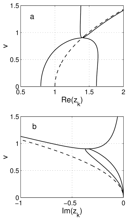
Figure 1: The evolution of $Re(z_{k})$ (a) and $Im(z_{k})$ (b),  $k=1,3$ (solid lines),  $k=2$ (dashed line), of the three eigenvalues of the effective Hamiltonian $H_{\rm eff}$ as a function of $v$ at $E=E_{c}=0.9847$. The parameters of the double DQ system are chosen as $\varepsilon_{1}=1,~{}\epsilon(L)=2-L/5,~{}u=1/4,~{}L=3$. At $v=v_{c}=0.9013$ the two eigenvalues $z_{1}$ and $z_{3}$ coalesce. The $Re(z_{1})$ and $Re(z_{3})$ approach each other when $v<v_{c}$, while the corresponding $Im(z_{1})$ and $Im(z_{3})$ bifurcate when $v>v_{c}$. At the branch point in the complex plane $E_{c}\neq E_{k},~{}E_{l}$.

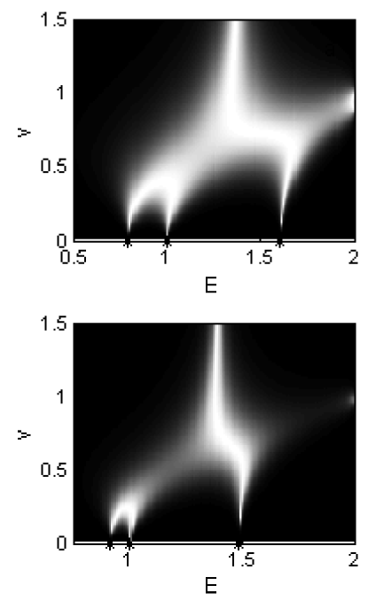
Figure 2: The transmission probability through the double QD versus $v$ and energy. Each single QD has one level at $\varepsilon_{1}=1$. It is $\epsilon(L)=2-L/5$ and $L=3$. The eigenenergies of the double QD are shown by stars. The case (a) corresponds to Fig. 1. The coupling constant between the single dots and the wire is $u=1/4$. The point of coalesced eigenvalues is $v_{c}=0.9013,~{}E_{c}=0.9847$, and the solutions of the fixed point equations (23) give $E_{k}=E_{l}\neq E_{c}$ as can be seen from Fig. 1. In the case (b), the coupling constant $u=u_{c}=0.1443$ between the single dots and the wire is chosen in correspondence to Eq. (30). Therefore, $E_{k}=E_{l}$ coincides with $E_{c}=7/5$ at $v=v_{c}$.

Let us consider now the behavior of the eigenvalues of the effective Hamiltonian as a function of $v$ at the energy $E=E_{k}$ where $E_{k}=Re(z_{k}(E_{k}))$ is solution of Eq. (23). In the general case, it is not easy to find the solution of the fixed point equation. However for the energy (28) at which the eigenvalues $z_{k}$ coalesce, Eq. (23) can be easily solved analytically. From (II), (27) and (28) we obtain

$$E_{k}=\epsilon(L_{c})=\frac{2(\epsilon(L_{c})-\varepsilon_{1}^{c})}{v_{c}^{2}}$$ (29)

and

$$u_{c}^{2}=\frac{(\epsilon(L_{c})-\varepsilon_{1}^{c})^{2}}{8}\left(\frac{4}{\epsilon(L_{c})^{2}}-1\right).$$ (30)

With the parameters chosen in Fig. 1, the last equation implies that solutions exist if $\epsilon(L)\leq 2$. We can consider therefore the evolution of the eigenvalues $z_{k}$ with $v$ at $E=E_{k}=\epsilon(L)=7/5$ and look for the point where the two eigenvalues coalesce. The critical values at the branch point in the complex plane are $u_{c}=0.1443$ and $E_{c}=7/5$. The evolution of the eigenvalues $z_{k}$ with $v$ for $u_{c},~{}E_{c},~{}L=3$ is similar to that given in Fig. 1. It is not shown here. The corresponding transmission picture Fig. 2 (b) is also similar to Fig. 2 (a). The main difference is the smaller spreading of the eigenvalues of $H_{B}$ and the smaller transmission probability according to the smaller value $u$ in the case with $E_{k}=E_{l}=E_{c}$. In both cases, the transmission is more spread in energy at $v<v_{c}$ than at $v\geq v_{c}$. This is in accordance with level repulsion seen in the eigenvalue trajectories at small $v$ and level attraction appearing at large $v$. There is a transmission peak at $v\approx 1$ near the upper border $E=2$ in both cases. This peak follows from the energy dependence of the $Re(z_{k})$: the positions of the two resonance states with large width approach $E=2$ with $v\approx 1$ (see Fig. 1 where the eigenvalues are shown for an energy $E<2$). We can state therefore that the characteristic features of the transmission pictures do not depend on whether the two states avoid crossing or cross in the complex plane.

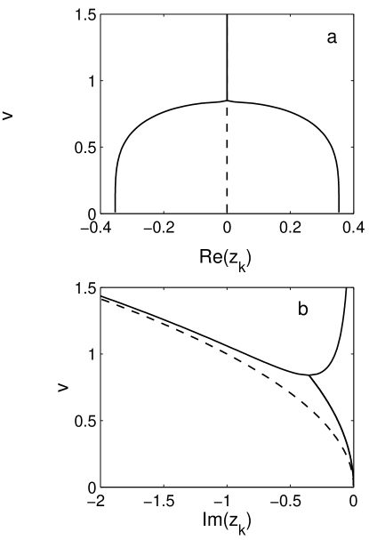
Figure 3: The evolution of $Re(z_{k})$ (a) and $Im(z_{k})$ (b),  $k=1,3$ (solid lines),  $k=2$ (dashed line), of the three eigenvalues of the effective Hamiltonian $H_{\rm eff}$ as a function of $v$ at $E=E_{c}=0$. The parameters $u=1/4,~{}L=10,~{}\varepsilon_{1}=0,~{}\epsilon(L)=2-L/5$ of the double QD system are chosen in such a manner that $\epsilon(L)=\varepsilon_{1}=0$ at $E=0$. Here, the two eigenvalues coalesce.  $v_{c}=8^{1/4}u^{1/2}=0.8409$.

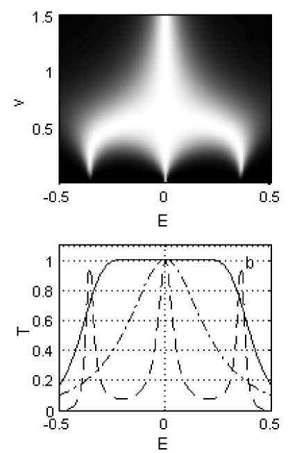
Figure 4: (a) The transmission probability through the double QD versus $v$ and energy for the case shown in Fig. 3. (b) The same as (a) but for fixed $v=0.2$ (dashed line), $v=0.53$ (solid line), and $v=0.83$ (dot-dashed line). At $v=0.53$, the double QD is a perfect filter.

In Fig. 3, we present the peculiar symmetrical behavior of the eigenvalues $z_{k}$ versus $v$ at $E=0$ for the resonant case with the parameters $\epsilon(L)=\varepsilon_{1},\;L=5$. In this case we have, according to Eqs. (27) and (28), $E_{c}=0$ and $v_{c}=8^{1/4}u^{1/2}$. At $v<v_{c}$, the widths of the two states 1 and 3 are equal, $Im(z_{1})=Im(z_{3})$, while at $v>v_{c}$ their positions are equal, $Re(z_{1})=Re(z_{3})$. The state 2 is not involved in the crossing scenario as in Fig. 1.

The transmission probability versus energy and $v$ is presented in Fig. 4. It has the same symmetrical behavior as the eigenvalue pictures. Of special interest is, as Fig. 4 (b) shows, that this symmetrical case is at $v=0.53$ a perfect filter: the transmission probability is equal to one in a large energy range.

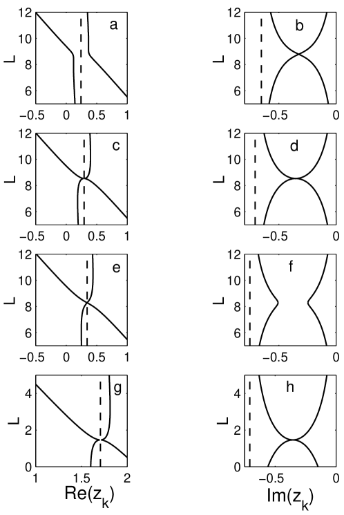
Figure 5: The evolution of the real and imaginary parts of the eigenvalues $z_{k}$,  $k=1,3$ (solid lines),  $k=2$ (dashed line), as a function of the length $L$ for the same double QD system as in Fig. 1 but $v=1$. $E_{c}=\pm\sqrt{2}$. The critical values of the length $L$ at the two points of coalescence of eigenvalues are $L_{1c}=1.4645,~{}L_{2c}=8.5355$. (a, b) $E=-\sqrt{2}-0.1$,  (c, d) $E=-\sqrt{2}$,  (e, f) $E=-\sqrt{2}+0.1$, and (g, h) $E=\sqrt{2}$.

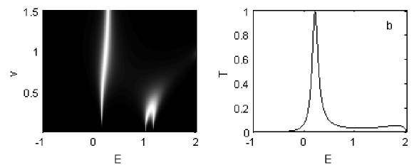
Figure 6: (a) The probability $T$ for transmission through the double QD versus $E$ and $v$ for $L_{c}=8.5355$. (b) The transmission probability as a function of $E$ for fixed $v=0.85$. It has one narrow peak on the background caused by the two broad resonance states. Parameters: $\varepsilon_{1}=1,~{}\epsilon(L)=2-L/5,~{}u=1/4$ as in Fig. 1.

Up to now, we traced the appearance of a branch point in the complex plane by enlarging the coupling strength $v$ between system and leads. In such a case, the branch points at which two eigenvalues coalesce, appear in a natural manner. It is less evident that the branch points in the complex plane can be seen in all parameters of the double QD system that define Eq. (27). We can take arbitrary but fixed values of $v$ and $u$ and consider the length $L$ or even the energy $E$ as a parameter in order to trace the coalescence of $z_{1}$ and $z_{3}$ at $L_{c}$ and $E_{c}$. The corresponding equations for achieving the coalescence are

$$\epsilon(L_{c})=\varepsilon_{1}^{c}\pm\sqrt{v_{c}^{4}-8u_{c}^{2}}\;;\qquad E_{c}=\pm\;\frac{2}{v_{c}^{2}}\;\sqrt{v_{c}^{4}-8u_{c}^{2}}\,.$$ (31)

A whole branch cut occurs along $L$ when $u=u_{c}$, $v=v_{c}$ and $E=E_{c}$ are fixed but $\varepsilon_{1}$ is not fixed. We consider in the following one branch point corresponding to a fixed value of $\varepsilon_{1}$.

The case with $L$ as a parameter is shown in Fig. 5 for the same double QD system as in Fig. 1, but $v=1$. There are two branch points in the complex plane corresponding to $E_{1c}=\sqrt{2},~{}L_{1c}=1.4645$ and $E_{2c}=-\sqrt{2},~{}L_{2c}=8.5355$. When $L<L_{1c}$ and $E>\sqrt{2}$, the two levels 1 and 3 avoid crossing as in the foregoing cases. In the region $L_{1c}<L<L_{2c}$ and $-\sqrt{2}<E<\sqrt{2}$, the levels do not cross at all in the complex plane due to their different widths: one of them is trapped by the other one due to the strong interaction via the continuum (i.e. via the modes propagating in the leads). For $L>L_{2c}$ and $E<-\sqrt{2}$, the levels again avoid crossing in the complex plane since the widths and with them the external coupling of the states via the continuum decrease in approaching $E=-2$.

The appearance of two branch points in the complex plane in Fig. 5 illustrates in a very convincing manner the interplay between internal and external interaction in approaching a branch point. In any case, a branch point separates regions with avoided level crossing ($L<L_{1c},~{}L>L_{2c}$) from those without any crossing of the levels ($L_{1c}<L<L_{2c}$) in the complex plane. One should underline, however, that the first branch point influences the physical observables such as the transmission probability [Fig. 6 (a)], indeed. The second branch point occurs as a threshold effect far from the energies $E_{1}$ and $E_{3}$ of the two states. The two eigenvalues $z_{1}$ and $z_{3}$ coalesce at the energy $E_{c}=-\sqrt{2}\ll E_{k}-\Gamma_{k}/2,E_{l}-\Gamma_{l}/2$, i.e. at the tails of the resonance states. This does not have any influence on the transmission probability.

In Fig. 6 (b), the transmission probability is shown at $L=L_{2c}$. It shows one peak, caused by the narrow resonance state, on the background created by the two broad resonance states. The narrow resonance is of Fano type by taking into account that the background decreases in approaching the two borders $E=\pm 2$. The transmission probability for other values of $L>L_{1c}$ is similar to that shown in Fig 6.

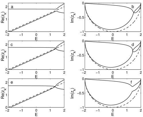
Figure 7: The evolution of the real (left column) and imaginary (right column) parts of the eigenvalues $z_{k}$,  $k=1,3$ (solid lines),  $k=2$ (dashed line), as a function of energy for transmission through the same double QD system as in Fig. 1, but $v=1$ as in Fig. 5. The point of coalesced eigenvalues is $E_{c}=\sqrt{2}$. The critical length is $L_{c}=1.4645$. (a,b) $L=L_{c}-0.1$, (c,d) $L=L_{c}$, and (e,f) $L=L_{c}+0.1$.

In Fig. 7, we show the analogue pictures for the $E$ dependence of the eigenvalues $z_{k}$. Due to the fact that the energy is bounded from below ($E=-2$) and above ($E=2$), the energy dependence of $Im(z_{k})$ can not be neglected. It is especially large for states that are strongly coupled to the continuum. While the energy dependence of $Im(z_{k})$ is more or less symmetrically around $E=0$, the $Re(z_{k})$ show an unsymmetrical behavior as a function of energy. It is of special interest, that the branch points in the complex plane appear also in the energy dependence of $Re(z_{k})$ and $Im(z_{k})$. An example is the branch point at $E_{c}=\sqrt{2},~{}L_{c}=1.4645$ that can be seen in Fig. 7.

IV Transmission through a double dot system with different coupling strengths to the two leads

Till now we considered the case that the double QD is coupled to the left and to the right reservoir with the same strength $v$. The couplings may be, however, different from one another. Such a case is interesting, also from a theoretical point of view, since the effective Hamiltonian becomes unseparable when the two coupling strengths differ from one another. This is in contrast to (7) where the double QD is assumed to be coupled symmetrically to the reservoirs and, according to (II) and (18), the eigenstate $|2)$ does not interfere with the other two states $|1)$ and $|3)$.

Following 1 we can write (1) as follows

$$\langle m|H_{\rm eff}|n\rangle = E_{m}\delta_{mn}+\sum_{C=L,R}\frac{1}{2\pi}\int_{-2}^{2}dE^{\prime}\frac{V_{m}(E^{\prime},C)V_{n}(E^{\prime},C)}{E+i0-E^{\prime}}$$ (32)

$$= E_{m}\delta_{mn}-\Big{(}v^{2}\psi_{m}(1)\psi_{n}(1)-w^{2}\psi_{m}(3)\psi_{n}(3)\Big{)}e^{ik},$$

where $v,w$ are the coupling strengths between the system and, respectively, the right and left reservoirs. Substituting the eigenstates of the closed double QD system (2) into (32) we obtain the following expression for the (symmetrical) effective Hamiltonian

$$H_{\rm eff}=\left(\begin{array}[]{ccc}E_{1}^{B}-\frac{(v^{2}+w^{2})u^{2}e^{ik}}{2\eta(\eta+\Delta\varepsilon)}&-\frac{u(v^{2}-w^{2})e^{ik}}{2\sqrt{\eta(\eta+\Delta\varepsilon)}}&\frac{u(v^{2}+w^{2})e^{ik}}{2\sqrt{2}\eta}\cr-\frac{u(v^{2}-w^{2})e^{ik}}{2\sqrt{\eta(\eta+\Delta\varepsilon)}}&\varepsilon_{1}-(v^{2}+w^{2})e^{ik}/2&\frac{u(v^{2}-w^{2})e^{ik}}{2\sqrt{\eta(\eta-\Delta\varepsilon)}}\cr\frac{u(v^{2}+w^{2})e^{ik}}{2\sqrt{2}\eta}&\frac{u(v^{2}-w^{2})e^{ik}}{2\sqrt{\eta(\eta-\Delta\varepsilon)}}&E_{3}^{B}-\frac{(v^{2}+w^{2})u^{2}e^{ik}}{2\eta(\eta-\Delta\varepsilon)}\cr\end{array}\right)\;.$$ (33)

The transmission probability for a system with different couplings of the double QD to the reservoirs demonstrates new features that appear when $v$ and $w$ differ strongly from one another (Fig. 8). In the calculations, we have chosen the following parameters for the double QD system: $\epsilon(L)=2-L/5,\;L=4,\;u=0.15,\;\varepsilon_{1}=1$. Then from (5) we have $E_{1}^{B}=0.8665,\;E_{2}^{B}=\varepsilon_{1}=1,\;E_{3}^{B}=1.3345$ for the three states of the closed system. The positions of the real parts $Re(z_{k}),k=1,2,3,$ of the three eigenvalues of the effective Hamiltonian $H_{\rm eff}$ are given in Fig. 8, left column, for $E=1.0,~{}0.92$ and 1.26.

Let us at first tune the energy of the incident particle to be resonant with the eigenenergy $E=E_{2}^{B}=1$ of the closed system. As it can be seen from Fig. 8 (a), we can have resonant transmission through the system at this energy only for $w<1/2$. Correspondingly, the transmission probability decreases for large $w$, Fig. 8 (b). Next, let us take $E=0.92$ that approaches $E_{1}$ for $w\approx 1/3$ according to Fig. 8 (c). Resonance transmission through the system is possible, at this energy, only when $w\geq 1/3$ and $v=0.06$. Since $Re(z_{1})$ is almost constant as a function of $w$ when $w>1/3$, also the transmission remains almost constant for $w>1/3$. Obviously the transmission is symmetrical relative to $v\leftrightarrow w$. As a result we obtain the peculiar picture of transmission probability shown in Fig. 8 (d). A similar picture is obtained if the energy is tuned to the third eigenenergy that is $E=E_{3}=1.26$ for large $w$, as shown in Figs. 8 (e, f). We mention, however, that at larger $u$ the transmission picture is less peculiar. Maximum transmission appears when $w\approx v$ and $v$ is about 2 or 3 times larger than $u$.

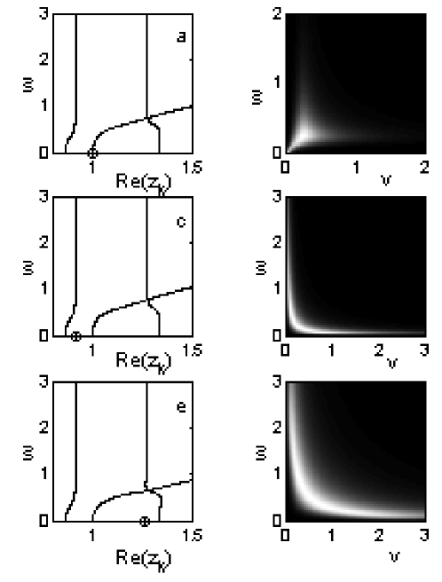
Figure 8: Left column: The evolution of the real parts of the eigenvalues of (32) as a function of $w$ for $v=0.1,~{}E=1.0$ (a),  $v=0.06,~{}E=0.92$ (c), and $v=0.1,~{}E=1.26$ (e). The parameters of the closed double QD system are $L=4,~{}u=0.15,~{}\varepsilon_{1}=1,~{}\epsilon(L)=2-L/5$. The circles at the x-axes denote the energies $E$. Right column: The transmission probability through the double QD versus coupling $v$ with the left reservoir and $w$ with the right reservoir. The energies $E$ are the same as in the corresponding figures of the left column.

V Transmission through a double dot system with more than three states

We show now results of some calculations for the transmission through a more realistic double QD system with more than one state in each of the single QDs. The number of propagating modes in the leads as well as in the wire, connecting the two single QDs, is restricted to one as in the foregoing calculations.

In Fig. 9, we show the transmission through such a double QD system with two states in each single QD as a function of energy $E$ and length $L$ for $u=0.25$ and for four different coupling strengths $v\leq 1$. The results show the change of the transmission picture as a function of $L$ for different $v$. At small $v$, the transmission takes place mainly at the energies $E_{k}^{B}$ of the discrete states of the double QD. This behavior is called usually resonant transmission. At larger $v$, however, the transmission peaks have nothing in common with the positions $E_{k}^{B}$ of the eigenstates of $H_{B}$. Here, the energy and $L$ dependence of the transmission follows basically that of the wave inside the wire, $\epsilon=3/2-L/7$. The transmission picture given in Fig. 9 corresponds to those shown in 1 . Transmission zeros appear for all $v$ at $E^{(0)}_{s}=(\varepsilon_{1}^{s}+\varepsilon_{2}^{s})/2$ where $\varepsilon_{k}^{s}~{}(k=1,2\,;~{}s=l,r)$  are the eigenenergies of, respectively, the left and right single QD. It is $E^{(0)}_{l}=E^{(0)}_{r}=3/4$ in Fig. 9.

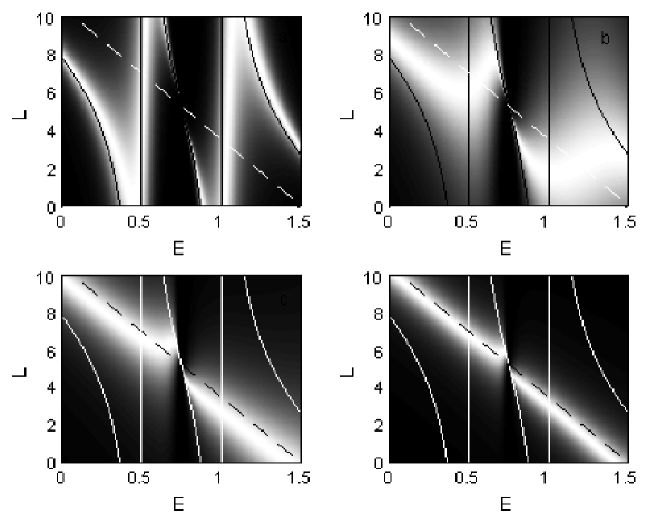
Figure 9: The transmission through a double QD versus $E$ and $L$ for $v=0.25$ (a),  0.5 (b),  0.75 (c) and 1.0 (d). The solid lines represent the five real eigenvalues $E_{k}^{B}$ of the Hamiltonian $H_{B}$ as a function of $L$. The dashed lines show the eigenenergy of the wire $\epsilon=3/2-L/7$. The eigenenergies of the two single QDs are equal: $\varepsilon_{1}=1/2,~{}\varepsilon_{2}=1$, and $u=0.25$. The transmission zero at $E_{0}=3/4$ is independent of $L$ and $v$.

The eigenvalue pictures corresponding to Fig. 9 are shown in Fig. 10. As long as $v$ is small, the energies $Re(z_{k})$ show a dependence on the parameter $L$ that is typical for interacting (discrete) states. The $Re(z_{k,l})$ of the two outermost states avoid crossing at a certain $L=L^{\rm cr}$ where the decay widths $2\,{Im}(z_{k,l})$ cross. At larger $v$, however, the eigenvalue pictures change since the widths of the two outermost states do no longer cross in the complex plane. Though the trajectories projected onto the energy axis cross at a certain value of $L$, the decay widths do not cross at all. This is due to the large difference between $Im(z_{1})$ and $Im(z_{3})$ as a consequence of resonance trapping (width bifurcation).

We can see from the eigenvalue trajectories Fig. 10 that the picture 9 (d) corresponds also to resonant transmission in spite of the fact that its structure is completely different from that in 9 (a). The point is that the eigenvalues of $H_{\rm eff}$ differ fundamentally from those of $H_{B}$ if the coupling of the states via the continuum is strong. The transmission peak appears at the position of a narrow resonance state. Besides this state, there are two broad and two narrow resonance states lying each very close to one another. The interferences between them are obviously destructive.

Another interesting result seen in Fig. 10 is that the decay width of the state in the middle of the spectrum vanishes at $L\approx 3$ for all $v$. At this value of $L$, the middle state crosses the energy $E^{(0)}=3/4$ where the transmission is zero. For a discussion of the transmission zeros see 1 .

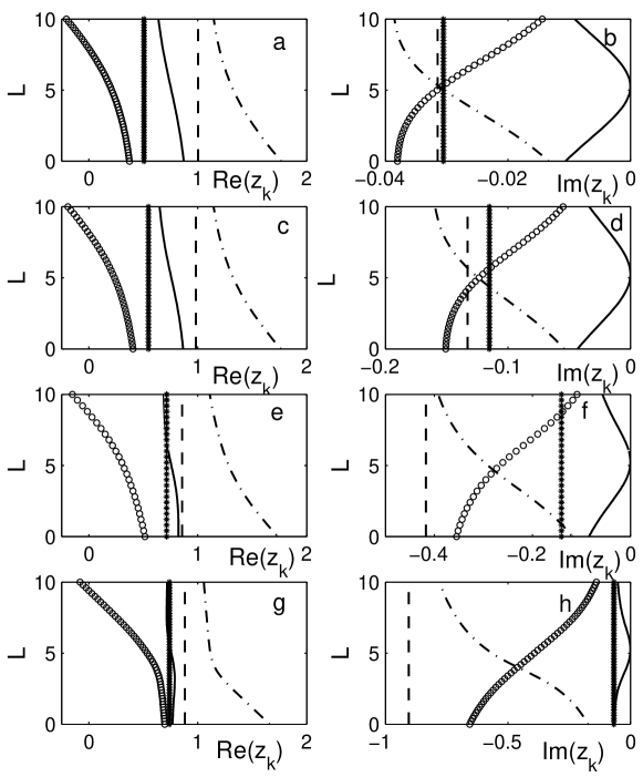
Figure 10: The evolution of real (left) and imaginary (right) parts of the five eigenvalues of the Hamiltonian $H_{\rm eff}$ as a function of the length $L$ for a double QD system. The coupling of the system to the continuum is $v=0.35$ (a, b),  0.8 (c, d), and  1.1 (e, f). The parameters of the system are $u=0.25$,  $E=0.25$,  $\epsilon=3/2-L/7$. The energies of the two single QDs are the same: $\varepsilon_{1}=1/2,~{}\varepsilon_{2}=1.$ The transmission of this double QD is shown in Fig. 9

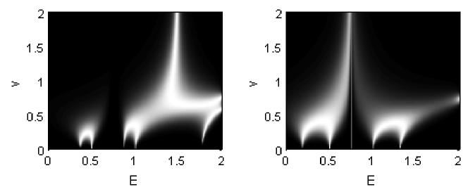
Figure 11: The transmission through a double QD versus $v$ and $E$ with the length $L=2$ (a) and 5 (b). The parameters are $u=0.25$,  $\epsilon(L)=2-L/4,~{}\varepsilon_{1}=1/2,~{}\varepsilon_{2}=1$. The transmission zero at $E_{0}=3/4$ is independent of $v$ and $L$.

In Fig. 11, the transmission through a double QD with altogether five states is shown as a function of energy and $v$ for two different lengths of the wire, $L=2$ and 5. Each of the two single QDs has two levels at $\varepsilon_{1}=1/2$ and $\varepsilon_{2}=1$, and the mode in the wire is $\epsilon(L)=2-L/4$. Transmission zeros appear at $E=3/4$ (for a detailed discussion of the transmission zeros see 1 ).

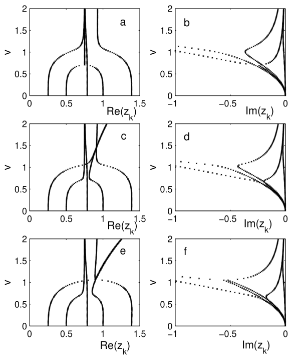
Figure 12: The evolution of real (left) and imaginary (right) parts of the five eigenvalues of the Hamiltonian $H_{\rm eff}$ as a function of the coupling strength $v$ for a double QD. The length of the wire is $L=0.7$ (a, b),  2 (c, d), and 3.03 (e,f). Parameters: $u=0.25$,  $E=0.75$,  $\epsilon(L)=2-L/4,~{}\varepsilon_{1}=1/2,~{}\varepsilon_{2}=1$. The transmission of this double QD is shown in Fig. 11.

The eigenvalue pictures corresponding to Fig. 11 at $E=0.75$ are shown in Fig. 12. We see a bifurcation of the widths as discussed in Sect. III as well as the corresponding branch points in the complex plane. At large $v$, there are two broad resonance states according to the two modes propagating in the two leads. The remaining three states are narrow at large $v$. They are trapped by the two broad states. As shown in Fig. 12, the two outermost states coalesce only at $L=3.03$. The resonance state in the middle of the spectrum coalesces, however, with another state at lower energy for all three lengths $L$ shown in Fig. 12.

The eigenvalue pictures calculated at different energies differ from one another in some details. The eigenvalue picture 12 corresponds to Fig. 1 calculated at a positive energy $E$. The two broad states are shifted to higher energy when $v$ is large. The shift is in the opposite direction when the eigenvalue pictures are calculated at negative energy. The calculation at $E=0$ gives a symmetrical picture corresponding to Fig. 3. In this case, the positions of all states at large $v$ are almost constant. The resonance trapping mechanism occurs symmetrically at $E=0$: the two outermost states coalesce at a somewhat higher value of $v$ than the two states lying nearer to the center of the spectrum. The state in the middle of the spectrum does not coalesce with any other state. It corresponds to the mode moving in the wire and is symmetrically coupled to the states at higher and at lower energy when $E=0$. This result corresponds completely to those shown in Figs. 3.

The figures show clearly that the transmission peaks appear at the positions of the eigenstates of $H_{B}$ only when $v$ is small. At larger $v$, the transmission is determined by interferences between the contributions from the different states. Nevertheless, it is resonant in relation to the eigenstates of the effective Hamiltonian $H_{\rm eff}$. Level repulsion at small $v$ and level attraction at large $v$ cause features of the transmission pictures for a double QD with altogether five states (Figs. 11 and 12) that are the same as those of a double QD with altogether only three states (Figs. 1 to 4). The only difference is the appearance of transmission zeros (Fig. 11) when the two single QDs are coupled to one another so that the double QD is effectively different from a 1d-chain as in Figs. 11 and 12, see 1 .

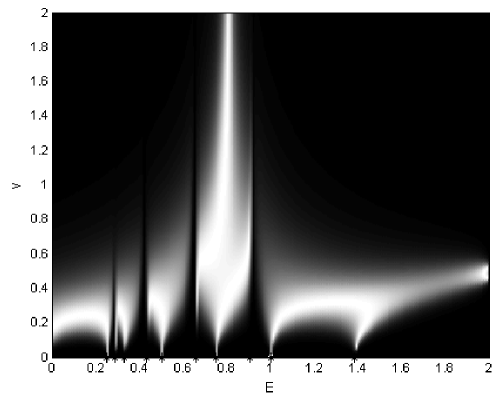
Figure 13: The transmission through a double QD versus $v$ and $E$ with the parameters $L=1.5$ and $u=0.2$. Each single QD has five levels at $\varepsilon_{i}=1/4,~{}1/3,~{}1/2,~{}3/4,~{}1$. The energy in the wire is $\epsilon=1-L/8$. The four transmission zeros are independent of $v$ and $L$.

In Fig. 13, the transmission through a QD with five states in each single QD is shown, and Fig. 14 gives the corresponding eigenvalue trajectories of all 11 states. The main features discussed for the cases with a smaller number of states remain. This holds true also for the transmission zeros the positions of which are determined by the energies of the eigenstates of the two single QDs. One of the differences to the cases with altogether three or five states is the following. The eigenenergy trajectories at $E=0$ are symmetrical around the energy $E=0$ in Fig. 3 with only one state in each single QD, while the symmetry is somewhat disturbed in Fig. 14 with more states in each single QD. In the latter case, the two outermost states do not approach each other completely. The lower state approaches one of the states out of the middle, and the upper state becomes trapped by these two states. As a consequence, the region with maximum transmission does not occur in the middle of the spectrum but at a somewhat lower energy. The reason for this asymmetry is the following: the functions $Re(z_{k})$ of ten states are raising with energy while all the $Im(z_{k})$ are vanishing at the two limits $E=\pm 2$ of the energy window (compare Fig. 7). Therefore, the widths of the states at lower energy are larger than those of the states at higher energy so that they trap the higher-lying states. For details of the resonance trapping phenomenon see rep .

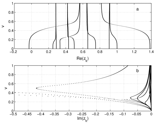
Figure 14: The evolution of the 11 eigenvalues $z_{k}$ of the effective Hamiltonian $H_{\rm eff}$ as a function of $v$ at $E=0$. (a) $Re(z_{k})$, (b) $Im(z_{k})$. $L=1.5,~{}u=0.2$. Each single QD has five levels at $\varepsilon_{i}=1/4,~{}1/3,~{}1/2,~{}3/4,~{}1$. The eigenenergy of the wire is $\epsilon=1-L/8$. The transmission of this double QD is shown in Fig. 13.

Common to all the pictures shown in this section is that the single-channel transmission through a double QD is of resonant character although its structure depends strongly on the strength $v$ by which the dot is coupled to the attached leads. The point is that the evolution of the eigenvalues of the effective Hamiltonian $H_{\rm eff}$ as a function of external parameters changes fundamentally at branch points in the complex plane. The transmission through the double QD shows a correspondingly sensitive dependence on the external parameters. Qualitative changes in the transmission picture are caused by branch points in the complex plane which separate the scenario with avoided level crossing from that without any crossing in the complex plane. While transmission occurs in the whole energy region with several peaks in the case with avoided level crossings, there is a smaller number of peaks of mostly different height in the case without any level crossings in the complex plane. The position of these peaks changes as a function of $L$. Common to both scenarios are only the $L$ independent transmission zeros (for a detailled discussion of the transmission zeros see 1 ).

The two coupling strengths $v$ and $u$ stand, respectively, for the coupling of the double QD as a whole to the leads (environment) and the coupling of the two single QDs to the wire (inside the double QD system). The ratio $v/u$ characterizes therefore the ratio between external and internal interaction of the states of an open quantum system. When the external coupling is much larger than the internal coupling, the external coupling of the levels via the modes propagating in the two leads, prevents the formation of a uniform QD. In the opposite case of large internal coupling, the relatively weak external coupling is unable to break the uniform QD. Most interesting is, of course, the transition region between the two different types of bonds in double QDs.

It is worthwhile to notice the following. The two levels that are the outermost ones of the spectrum, cross or avoid crossing in the complex plane at $E=0$. The distance in energy to the crossing or avoided crossing, that occurs between two other levels, is smaller than their decay widths. That means, effectively all states are involved in the scenario of avoided level crossing in the complex plane.

Additionally, we mention that the dependence of the transmission on the length $L$ of the wire is determined by the manner the wave propagates inside the wire. It can be replaced by another relation between $\epsilon$ and $L$ than that used in our calculations or by the analogue relation between $\epsilon$ and the width $d$ of the wire. In the last case, $L$ can be kept constant in studying the dependence of the transmission from $d$, see the discussion at the end of Ref. 1 .

VI Summary

The results considered in the present paper are obtained in the formalism worked out in 1 for the description of a double QD system. The formalism is based on the $S$ matrix theory with use of the effective Hamiltonian that describes the spectroscopic properties of the open quantum system. The formalism is applied in 1 to the description of transmission zeros in the conductance through double QDs. These zeros are determined by the spectroscopic properties of the constituents of the double dot system and by the manner the single QDs are coupled. They appear at all ratios $v/u$ of the coupling strengths. Our present study is devoted, above all, to the transmission peaks. Their positions and widths depend on the ratio $v/u$ and are influenced by branch points in the complex plane. At these points, the transition between the two scenarios with avoided level crossing and no crossing in the complex plane takes place. In any case, the transmission is resonant.

As long as $v/u$ is small, the levels repel in energy (as the discrete eigenstates of $H_{B}$) and the decay widths of the different states are of comparable value. This causes some spreading of the transmission probability over a relatively large energy region. At large $v/u$, however, the levels attract in energy and the decay widths bifurcate. This causes transmission peaks at the positions of the narrow states that appear on the smooth background created by the broad states. The positions of the transmission peaks depend, in this case, strongly on the length of the wire or on another parameter that controls the propagation of the mode inside the wire. The two different scenarios are separated by a branch point in the complex plane. At such a point, two eigenvalues ($z_{k}$ and $z_{l}$) of the effective Hamiltonian coalesce at the energy $E=E_{c}$. Sometimes, $E_{c}=E_{k}=E_{l}$. Mostly however $E_{k}\neq Re(z_{k})|_{E=E_{c}}$ and $E_{l}\neq Re(z_{l})|_{E=E_{c}}$, and the branch point in the complex plane is not a double pole of the $S$ matrix.

We underline that the resonance phenomena appearing in the transmission through double QDs are the same as those observed in, e.g., the scattering on nuclei or atoms rep . The role of the branch points in the complex plane for the transmission through a double dot system agrees with that discussed in a schematical study ro01 and for a double-well system vanroose . In our model double QD, however, the energy dependence of the eigenvalues $z_{k}$ of the effective Hamiltonian $H_{\rm eff}$ is relatively strong. Especially $Im(z_{k})$ shows a strong energy dependence due to the energy window with thresholds at a lower and an upper finite energy. The spectrum is therefore bounded from below and from above, and the eigenvalues of the effective Hamiltonian cannot satisfyingly be approximated by the poles of the $S$ matrix.

The results discussed here are true for single-channel transmission through a double QD system that consists of two single QDs with similar energy spectra and a narrow wire that couples the two single QDs and allows the propagation of only one mode. When the energy spectra of the two single QDs are very different from one another and the coupling strength $u$ to the wire is small, the transmission picture at large $v$ differs from that discussed above. In such a case, the transmission is hindered at large $v$, above all due to the energy gap between the levels of the two single QDs through which the transmission takes place.

In the present paper, the behavior of a simple model is considered that reflects many characteristic features of realistic double QDs with more complicated structure, see 1 . The results obtained may guide the construction of double QDs. The position of transmission zeros and transmission peaks can be controlled by varying the coupling strengths $v$ and $u$ as well as the propagation of the mode inside the wire. An example is the broad plateau with maximal transmission shown in Fig. 4 (b). Using the interplay between internal and external interaction allows to control the properties of QDs in a systematic manner.

References

- (1) T. Kato, Perturbation Theory of Linear Operators (Springer, Berlin 1966).
- (2) N. Moiseyev, Phys. Rep. 302, 211 (1998).
- (3) I. Rotter, Phys. Rev. E 64, 036213 (2001).
- (4) F.M. Dittes, W. Cassing and I. Rotter, Z. Phys. A 337, 243 (1990); I. Rotter, Rep. Prog. Phys. 54, 635 (1991).
- (5) M. Müller, F.M. Dittes, W. Iskra, and I. Rotter Phys. Rev. E 52, 5961 (1995).
- (6) A.I. Magunov, I. Rotter, and S.I. Strakhova, J. Phys. B: At. Mol. Opt. Phys. 32, 1669 (1999); J. Phys. B: At. Mol. Opt. Phys. 34, 29 (2001).
- (7) J. Okołowicz, M. Płoszajczak, and I. Rotter, Phys. Rep. 374, 271 (2003).
- (8) E. Narevicius and N. Moiseyev, Phys. Rev. Lett. 84, 1681 (2000); J. Chem. Phys. 113, 6088 (2000).
- (9) R.G. Newton, Scattering Theory of Waves and Particles, Springer, New York, 1982.
- (10) O. Latinne, N.J. Kylstra, M. Dörr, J. Purvis, M. Terao-Dunseath, C.J. Joachain, P.G. Burke, and C.J. Noble, Phys. Rev. Lett. 74, 46 (1995).
- (11) N.J. Kylstra and C.J. Joachain, Europhys. Lett. 36, 657 (1996); Phys. Rev. A 57, 412 (1998).
- (12) W. Vanroose, P. Van Leuven, F. Arickx, and J. Broeckhove, J. Phys. A: Math Gen. 30, 5543 (1997).
- (13) W. Vanroose, Phys. Rev. A 64, 062708 (2001).
- (14) T. Meier, A. Schulze, P. Thomas, H. Vaupel, and K. Maschke, Phys. Rev. B 51, 13977 (1995).
- (15) A.I. Magunov, I. Rotter, and S.I. Strakhova, Phys. Rev. B 68, 245305 (2003).
- (16) I. Rotter and A.F. Sadreev, cond-mat/0403184 (2004).
- (17) W.G. van der Wiel, S. De Franceschi, J.M. Elzerman, T. Fujisawa, S. Tarucha, and L.P. Kouwenhoven, Rev. Mod. Phys. 75, 1 (2003).
- (18) J.P. Bird, R Akis, D.K. Ferry, A.P.S. de Moura, Y.-C. Lai, and K.M. Indlekofer, Rep. Progr. Phys. 66, 1 (2003).
- (19) A.F. Sadreev and I. Rotter, J. Phys. A: Math. Gen. 36, 11413 (2003).
- (20) F. Keck, H.J. Korsch, and S. Mossmann, J. Phys. A: Math. Gen. 36, 2125 (2003).