Geometric Phases for Mixed States during Cyclic Evolutions

Abstract

The geometric phases of cyclic evolutions for mixed states are discussed in the framework of unitary evolution. A canonical one-form is defined whose line integral gives the geometric phase which is gauge invariant. It reduces to the Aharonov and Anandan phase in the pure state case. Our definition is consistent with the phase shift in the proposed experiment [Phys. Rev. Lett. 85, 2845 (2000)] for a cyclic evolution if the unitary transformation satisfies the parallel transport condition. A comprehensive geometric interpretation is also given. It shows that the geometric phases for mixed states share the same geometric sense with the pure states.

When a pure quantal state undergoes a cyclic evolution the system returns to its original state but may acquire a nontrivial phase factor of purely geometric origin. This was first discovered by Berry berry in the adiabatic context, and generalized to non-Abelian by Wilczek and Zee nona . A nice interpretation was given by Simon simon in terms of a natural Hermitian connection, as the parallel transport holonomy in a Hermitian line bundle. Extension to the nonadiabatic cyclic case was given by Aharonov and Anandan aa . Based on Pancharatnam’s earlier work on interference of light pan , this concept was generalized to noncyclic evolutions and nonunitary evolutions nonc1 ; nonc2 . The geometric phases for entangled states have also been discussed ent . Applications of the geometric phase have been found in molecular dynamics ek11 , response function of the many-body system ek12 , and geometric quantum computation ek14 . In all these developments the geometric phases have been discussed only for pure states. However, in some applications we are interested in mixed state cases ek14 ; Ekert .

Uhlmann was probably the first to address the issue of mixed state in the context of purification, but as a purely mathematical problem ulman1 . Recently, Sjöqvist et al. Ekert gave a new formalism of the geometric phase for mixed state in the experiment context of quantum interferometry under parallel transport condition. It has been pointed out com that the latter geometric phase can be undefined at nodal points in the parameter space where the interference visibility vanishes. Anyway, the geometric phases for mixed states proposed in Refs. ulman1 and Ekert are generically different in the unitary case and match only under very special conditions such as in terms of pure states umek .

In this paper, we give a definition of geometric phase for a cyclic evolution of mixed quantal state in the dynamical context of quantum system. The reasons of employing the cyclic evolution are two: (i) the cyclic evolution of a physical system is of the most interest in physics both experimentally and theoretically (ii) the phase shift in a cyclic evolution should be definite. Firstly, we give a straightforward generalization of Aharonov and Anandan (A-A) phase for the global cyclic evolution where the total phase is explicit. Though this case seems a trivial extension of (A-A) phase, it contains the essence of geometric phase of mixed state. Then, we give the discussion of the general case based on a definition of the total phase. This geometric phase reduces to the (A-A) phase aa , the standard geometric phase for pure state undergoing a cyclic evolution. We find that if the evolution satisfies the parallel transport condition the geometric phase is consistent with the result in Ref. Ekert . Moreover, we give the geometric meaning of the geometric phases of mixed states which share the same sense with the pure states for the first time.

Supposing a quantum system with the Hamiltonian $H(t),$ the density operator $\rho(t)$ of this system will undergo the following evolution

$$\rho(t)=U(t)\rho(0)U^{+}(t),$$ (1)

where $U(t)=\mathbf{T}e^{-i\int_{0}^{t}H(t^{\prime})dt^{\prime}/\hbar}$ is a unitary transformation, here $\mathbf{T}$ is the chronological operator. If $U(\tau)$ and $\rho(0)$ are commutative: $[U(\tau),\rho(0)]=0,$ i.e., $\rho(\tau)=\rho(0),$ we say this state undergoes a cyclic evolution with period $\tau$. Furthermore, if $U(\tau)=e^{i\phi}I$, this evolution can be called the global cyclic evolution since for any $\rho(0)$ we have $\rho(\tau)=\rho(0).$

At first, we study the case of the global cyclic evolution. Now define $\widetilde{U}(t)=e^{-i\phi(t)}U(t)$ such that $\widetilde{U}(\tau)=I.$ We define the geometric phase for such state during the global cyclic evolution as

$$\phi_{g}=i\int_{0}^{\tau}Tr\left[\rho(0)\widetilde{U}^{+}(t)\frac{d\widetilde{U}(t)}{dt}\right]dt.$$ (2)

Using the transformation between $\widetilde{U}(t)$ and $U(t),$ one can have

$$\phi_{g}=\phi-\phi_{d},$$ (3)

and

$$\phi_{d} = -i\int_{0}^{\tau}dtTr\left[\rho(0)U^{+}(t)\frac{dU(t)}{dt}\right]$$

$$= -\frac{1}{\hbar}\int_{0}^{\tau}dtTr\left[\rho(t)H(t)\right].$$

Obviously $\phi_{d}$ is just the dynamical phase during the cyclic evolution.

We can prove that if $\rho(t)$ is the density operator of a pure state the geometric phase defined by Eq. (2) is just the Aharonov and Anandan phase aa . Assuming $\rho(0)=\left|\psi(0)\right\rangle\left\langle\psi(0)\right|,$ $\left|\psi(t)\right\rangle=U(t)\left|\psi(0)\right\rangle$. Let $\left|\varphi(t)\right\rangle=e^{-i\phi(t)}\left|\psi(t)\right\rangle,$ then we have $\left|\varphi(t)\right\rangle=\widetilde{U}(t)\left|\varphi(0)\right\rangle.$ So, the Eq. (2) can be written as $\phi_{g}=i\int_{0}^{\tau}\left\langle\varphi(t)\right|\left.\dot{\varphi}(t)\right\rangle dt$ which is just the result of Ref. aa .

An initial state can always be diagonalized, namely,

$$\rho(0)=\sum\limits_{k}w_{k}\left|k\right\rangle\left\langle k\right|,$$ (5)

where $\left|k\right\rangle$ are bases for the system and $w_{k}$ are classical probability to find a member of the ensemble in the corresponding state. For the global cyclic evolution we have $U(\tau)\left|k\right\rangle=e^{i\phi}$ $\left|k\right\rangle,$ then the A-A phase of $\left|k\right\rangle$ is $\phi_{g}^{k}=\phi-\phi_{d}^{k}$, where $\phi_{d}^{k}=$ $-\frac{1}{\hbar}\int_{0}^{\tau}dtTr\left[\left|k\right\rangle\left\langle k\right|U^{+}(t)\dot{U}(t)\right].$ Substituting (5) into (Geometric Phases for Mixed States during Cyclic Evolutions), and from (3) we obtain

$$\phi_{g}=\phi-\sum\limits_{k}w_{k}\phi_{d}^{k}=\sum\limits_{k}w_{k}\phi_{g}^{k}.$$ (6)

So, for the global cyclic evolution the geometric phases of mixed states have explicit meanings: the geometric phases of a mixed state is the weighted average of the geometric phases of the constitute pure states.

Example I. –Suppose that a qubit (a spin-$\frac{1}{2}$ particle) with a magnetic moment is in a homogenous magnetic field $\mathbf{B}$ along the $z$ axis. Then the Hamiltonian in the rest frame is $H=-\mu B\sigma_{z}.$ Suppose the initial state is

$$\rho(0)=\frac{1}{2}[I+r(\sin\theta\sigma_{x}+\cos\theta\sigma_{z})],$$ (7)

where $r$ is a constant and $0\leq r\leq 1$. So we have $\rho(t)=U(t)\rho(0)U^{+}(t)$ with

$$U(t)=\exp(i\mu Bt\sigma_{z}/\hbar).$$ (8)

This unitary evolution is periodic with period $\tau=\pi\hbar/\mu B$, i.e., $\rho(\tau)=\rho(0).$ It is easy to see that $U(\tau)=\exp(i\pi)I.$ Let $\widetilde{U}(t)=e^{-i\mu Bt/\hbar}U(t),$ then $\widetilde{U}(\tau)=U(0).$ From Eq. (2), and after some elaboration we can obtain the geometric phase

$$\phi_{g}=\pi(1-r\cos\theta).$$ (9)

Obviously, if $r=1,$ we get $\phi_{g}=\pi(1-\cos\theta)$ which is just the A-A phase aa .

On the other hand, we can have two pure states $\rho_{1}(0)=\frac{1}{2}[I+(\sin\theta\sigma_{x}+\cos\theta\sigma_{z})]$ and $\rho_{2}(0)=\frac{1}{2}[I+(\sin(\pi+\theta)\sigma_{x}+\cos(\pi+\theta)\sigma_{z})],$ which can construct a set of orthonormal bases.  From (7), we have $\rho(0)=\frac{1+r}{2}\rho_{1}(0)+\frac{1-r}{2}\rho_{2}(0).$ Obviously, this is a diagonal representation of the initial state $\rho(0).$ Then from Eq.(6), we can obtain $\phi_{g}=\frac{1+r}{2}\pi(1-\cos\theta)+\frac{1-r}{2}\pi(1-\cos(\pi+\theta))=\pi(1-r\cos\theta).$

The above discussion of the general cyclic evolution seems a trivial extension of (A-A) phase, but it contains the essence of geometric phase of mixed state.

For the general case of a cyclic evolution, the density matrix and transformation satisfy $[U(\tau),\rho(0)]=0.$ We can not find the total phase explicitly from this condition. To factor out the total phase, we use the Pancharatnam’s brilliant idea, i.e., the Pancharatnam connection pan . We define the total phase of the mixed state during a cyclic evolution with the initial state $\rho(0)$ and the unitary transformation $U(t)$ as

$$\phi=\arg Tr[\rho(0)U(\tau)].$$ (10)

Let $\widetilde{U}(t)=e^{-i\phi(t)}U(t)$ such that $\phi(\tau)=\phi.$ Based on this definition, the geometric phase of the cyclic evolution can be also defined by Eq. (2). Obviously, the geometric phase for a cyclic evolution takes the same form as in Eq. (3). Indeed Eq. (2) defines a canonical one-form in the parameter space:

$$\beta=iTr\left[\rho(0)\widetilde{U}^{+}(t)d\widetilde{U}(t)\right].$$ (11)

It is not difficult to prove that $\beta$ is a real number. The geometric phase can be obtained by its line integral, i.e.,

$$\phi_{g}=\oint\beta.$$ (12)

The equivalent of the above formula for the pure states case is well-known pg ; nonc2 .

The geometric phase defined above is manifestly gauge invariant: it does not depend on the dynamics, but it depends only on the geometry of the close unitary path given by the unitary transformation $U(t).$ Assuming $\alpha$ is a dynamic parameter of this system, the nature of the cyclic evolution requires $\alpha(0)=\alpha(\tau)$ berry . Under the transformation $\widetilde{U}(t)^{\prime}=e^{i\delta(\alpha)}\widetilde{U}(t),$ we can have $\beta^{\prime}=\beta-d\delta.$ It is easy to prove that $\oint\beta^{\prime}=\oint\beta$ since $\delta(a(\tau))=\delta(a(0)).$ Indeed the quantity $\beta=iTr[\rho(0)\widetilde{U}^{+}(t)d\widetilde{U}(t)]$ can be regarded as a gauge potential on the space of density operators pertaining to the system.

Example II. –Consider a spin-$\frac{1}{2}$ particle is initially in the state

$$\rho(0)=\frac{1}{2}(I+r\sigma_{z}),\;$$ (13)

where $r\leq 1$ is a constant. Suppose this particle is in a magnetic field $\mathbf{B}(t)$ with

$$\mathbf{B}(t)=\left\{\begin{array}[]{cc}-(\omega\hbar/\mu)\widehat{e}_{y},&0\leq t\leq t_{1}\\ -(\omega\hbar/\mu)\widehat{e}_{z},&t_{1}\leq t\leq t_{2}\\ -(\omega\hbar/\mu)(\sin\varphi\widehat{e}_{x}-\cos\varphi\widehat{e}_{y}),&t_{2}\leq t\leq\tau\end{array}\right.,$$ (14)

in which $\omega$ is a constant and $t_{1}=\frac{\theta}{2\omega},$ $t_{2}=$ $\frac{\theta+\varphi}{2\omega}$ and $\tau=\frac{2\theta+\varphi}{2\omega}.$ So, the unitary transformation is

$$U(t)=\left\{\begin{array}[]{cc}e^{-i\omega t\sigma_{y}},&0\leq t\leq t_{1}\\ e^{-i\omega(t-t_{1})\sigma_{z}}e^{-i\frac{\theta}{2}\sigma_{y}},&t_{1}\leq t\leq t_{2}\\ \begin{array}[]{c}e^{-i\omega(t-t_{2})(\sin\varphi\sigma_{x}-\cos\varphi\sigma_{y})}\\ \times e^{-i\frac{\varphi}{2}\sigma_{z}}e^{-i\frac{\theta}{2}\sigma_{y}},\end{array}&t_{2}\leq t\leq\tau\end{array}\right..$$ (15)

Then, $U(\tau)=e^{-i\frac{\theta}{2}(\sin\varphi\sigma_{x}-\cos\varphi\sigma_{y})}e^{-i\frac{\varphi}{2}\sigma_{z}}e^{-i\frac{\theta}{2}\sigma_{y}}.$ We can prove that $U(\tau)\rho(0)U^{+}(\tau)=\rho(0).$ Under this unitary transformation, the state undergos a cyclic evolution with a closed path of the corresponding Bloch vector as showing in Fig.1, where the vectors at points $B$ and $C$ are $\mathbf{r}_{B}=(r\sin\theta,0,r\cos\theta)$ and $\mathbf{r}_{C}=(r\sin\theta\cos\varphi,r\sin\theta\sin\varphi,r\cos\theta)$ respectively. From Eq. (10) and (Geometric Phases for Mixed States during Cyclic Evolutions), we have the total phase of this cyclic evolution: $\phi=-\arctan\left[r\tan\frac{\varphi}{2}\right],$ and the dynamic phase: $\phi_{d}=-\frac{\varphi}{2}r\cos\theta.$ Then, the geometric phase of this cyclic evolution is

$$\phi_{g}=-\arctan\left[r\tan\frac{\varphi}{2}\right]+\frac{\varphi}{2}r\cos\theta.$$ (16)

We know that if $\theta=\frac{\pi}{2}$ the closed path on the Bloch sphere is geodesic ek21 , i.e., the dynamical phase is zero. At this time the geometric phase is $-\arctan\left[r\tan\frac{\varphi}{2}\right],$ which has also been pointed out in Ref. Ekert and verified by the recent experimental observations exp .

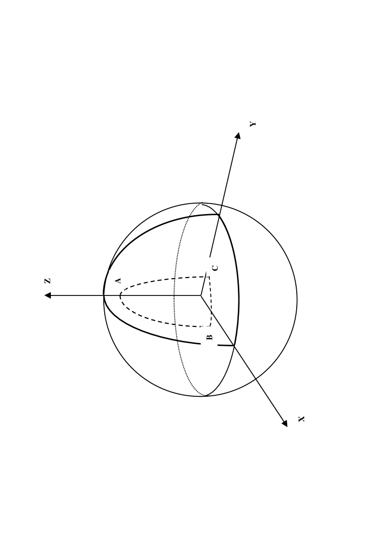
Figure 1: Path with cyclic evolution of the Bloch vector. The solid line represents a geodesic path of the unitary pure state case and defines a spherical triangle enclosing the solid angle $\pi/2.$ The dashed line represents the closed path of the mixed state with the unitary evolution defined by (15), where the initial state is given in Eq. (13).

If $\varphi=2\pi,$ i.e., the points $B$ and $C$ in Fig. 1 are the same. Obviously, the geometric phase for such a path should be equal to the case in Example I except for the direction of magnetic field reversed. From (16), we have $\phi_{g}=\pi(1+r\cos\theta)$ which is consistent with Eq. (9).

From our definition of the geometric phase, we can get a theorem for a composite quantum system.

Theorem: Let $\rho^{AB}$ be a density operator of a composite quantum system of $A$ and $B$.  If the system evolves under the unitary transformation $U(t)=I^{A}$ $\otimes U^{B}$ with $U^{B}=\mathbf{T}e^{-i\int_{0}^{t}H(t^{\prime})dt^{\prime}/\hbar}$ and $[\rho^{AB},U(\tau)]=0$, then the geometric phase of such a composite system equals to one of the subsystem $B,$ i.e., $\phi_{g}^{AB}=\phi_{g}^{B}.$

The density operator of such system can be expressed by

$$\rho^{AB} = \frac{1}{N_{A}N_{B}}[I^{A}\otimes I^{B}+\mathbf{r}^{A}\cdot\vec{\lambda}^{A}\otimes I^{B}$$ (17)

$$+I^{A}\otimes\mathbf{r}^{B}\cdot\vec{\lambda}^{B}+\beta_{ij}\lambda_{i}^{A}\otimes\lambda_{j}^{B}],$$

where $N_{A}$ and $N_{B}$ are the orders of density matrices for each subsystems, $\vec{\lambda}^{A}=(\lambda_{i}^{A};i=1,2,\cdots,N_{A}^{2}-1)$ and $\vec{\lambda}^{B}=(\lambda_{i}^{A};i=1,2,\cdots,N_{B}^{2}-1)$ are the generators of $SU(N_{A})$ and $SU(N_{B})$ respectively, $\mathbf{r}^{A}=(r_{i}^{A};i=1,2,\cdots,N_{A}^{2}-1)$ and $\mathbf{r}^{B}=(r_{i}^{B};i=1,2,\cdots,N_{B}^{2}-1)$ are two vectors, and $\beta_{ij}$ are $(N_{A}^{2}-1)(N_{B}^{2}-1)$ real numbers. Because $Tr(\lambda_{i}^{A,B})=0,$ one can have $\phi^{AB}=\arg Tr[\rho^{AB}U(\tau)]=\arg Tr[\rho^{B}U^{B}(\tau)]$ where $\rho^{B}$ is reduced density operator for $B,$ i.e., $\rho^{B}=\frac{1}{N_{B}}[I^{B}+$ $\mathbf{r}^{B}\cdot\vec{\lambda}^{B}]$. From (Geometric Phases for Mixed States during Cyclic Evolutions), we can also obtain $\phi_{d}^{AB}=-i\int Tr[\rho^{AB}U^{+}(t)\dot{U}(t)]=-i\int Tr[\rho^{B}U^{B^{+}}(t)\dot{U}^{B}(t)]$. So the geometric phase for $\rho^{AB}$ is $\phi_{g}^{AB}=\phi^{AB}-\phi_{d}^{AB}$ $=\phi^{B}-\phi_{d}^{B}$, where $\phi^{B}=\arg Tr[\rho^{B}U^{B}(\tau)]$ and $\phi_{d}^{B}=-i\int Tr[\rho^{B}U^{B^{+}}(t)\dot{U}^{B}(t)].$ The geometric phase of the subsystem $B$ is $\phi_{g}^{B}$ $=\phi^{B}-\phi_{d}^{B}=\phi_{g}^{AB}.$

We know that for a pure state of an entangled composite quantum system $\rho^{AB},$ the reduced density operators $\rho^{A,B}$ are mixed states. So this theorem may have some important applications, at least to observe the geometric phase for mixed state, since the geometric phase for a pure state can be acquired by methods known before.

Recently, Sjöqvist et al. have also proposed geometric phases for mixed states under the parallel transport condition Ekert . If the unitary transformation $U(t)$ satisfies a parallel condition we can prove the geometric phase given by Eq. (2) is consistent with what was obtained in Ref. Ekert . The parallel transport condition for a mixed state undergoing unitary evolution is

$$Tr[\rho(t)U^{+}(t)\dot{U}(t)]=0.$$ (18)

Under this condition, from the definition in Ref. Ekert the geometric phase of the cyclic evolution can be expressed as $\overline{\phi}_{g}=\arg Tr[\rho(0)U(\tau)].$

Indeed, for the unitary operator $U(t)$ we can always obtain another unitary operator by a $U(1)$ transformation, $U^{\prime}(t)=e^{i\xi(t)}U(t),$ so that $Tr[\rho(t)U^{\prime+}(t)\dot{U}^{\prime}(t)]=0.$ From this condition, it is easy to prove that

$$\dot{\xi}(t)=iTr[\rho(0)U^{+}(t)\dot{U}(t)].$$ (19)

So $\xi(\tau)=-\phi_{d}.$ From (10) and (3), $\phi_{g}=\arg Tr[\rho(0)U(\tau)]+\xi(\tau)=\arg Tr[\rho(0)U^{\prime}(\tau)].$ Obviously, such a parallel transport $U^{\prime}(\tau)$ is unique for an initial state $\rho(0)$ and the unitary operator $U(t)$. So, if $U(t)$ satisfies the parallel transport condition, the dynamical phase in Eq. (3) vanishes identically, so $\overline{\phi}_{g}=\phi_{g},$ i.e., under the parallel transport condition our definition of the geometric phase is consistent with the definition in Ref. Ekert .

However, for an initial state $\rho(0)$ and the unitary operator $U(t),$ one can construct alternative parallel transport by a unitary transformation, except for a $U(1)$ transformation, i.e., the parallel transport corresponding the initial state and the unitary operator $U(t)$ is not unique Ekert ; cond . We must emphasize that only for the parallel transport obtained by the $U(1)$ transformation (which is unique), $U^{\prime}(\tau)=e^{i\xi(t)}U(t)$ determined by Eq. (19), the geometric phase can be expressed as $\phi_{g}=\arg Tr[\rho(0)U^{\prime}(\tau)]$. As an example, we consider the case of Example I. For the state $\rho(0)$ given in (7), one can have two pure states $\rho_{\pm}=\frac{1}{2}[I\pm(\sin\theta\sigma_{x}+\cos\theta\sigma_{z})]$ such that $\rho(0)=\frac{1+r}{2}\rho_{+}+\frac{1-r}{2}\rho_{-}.$ For the unitary operator $U(t)=\exp(i\mu Bt\sigma_{z}/\hbar),$ by unitary transformation $e^{-i[\mu Bt(\cos\theta)(\sin\theta\sigma_{x}+\cos\theta\sigma_{z})/\hbar]},$ we can construct $U^{\prime\prime}=e^{i(\mu Bt\sigma_{z}/\hbar)}e^{-i[\mu Bt(\cos\theta)(\sin\theta\sigma_{x}+\cos\theta\sigma_{z})/\hbar]}$ which satisfies $Tr[\rho_{\pm}(U^{\prime\prime})^{+}\dot{U}^{\prime\prime}(t)]=0.$ Obviously, this is a parallel transport of $\rho(t)=U^{\prime\prime}(t)\rho(0)U^{\prime\prime^{+}}(t)=U(t)\rho(0)U^{+}(t).$ It is easy to obtain $\arg Tr[\rho(0)U^{\prime\prime}(\tau)]=\pi-\arctan[r\tan(\pi\cos\theta)]$ which does not equal to the geometric phase given by Eq. (9).

In fact, the set of the density operators constructs a base space $\mathcal{M}$ (the subspace corresponding to pure states is isomorphic to the projective Hilbert space). The unitary transformations $U$ just define a line bundle $\mathcal{F}$ on the base space with the projection map $\Pi$ as $\Pi^{-1}(\rho)=\{\rho:\rho\rightarrow c=Tr(U\rho)/|Tr(U\rho)|,\;c$ $\in U(1)\}$. Then the cyclic evolution discussed in the present paper is just define a closed curve $\mathit{C}:[0,\tau]\rightarrow\mathcal{M}$ on the base space, but on the bundle space the path is not closed with the final point lifted by a $U(1)$ factor $c(\tau).$ On the other hand, using $U(1)$ transformations, we can always obtain a unitary transformation $U^{\prime}(t)$ determined by Eq. (19) which satisfies the parallel transport condition for a given closed path $C.$ Then, the geometric phase defined in Eq. (3) can be expressed by the phase factor of the parallel lift : $\phi_{g}=\arg Tr[\rho(\tau)U^{\prime}(\tau)]$. Under this consideration the geometric phases of mixed states share the same geometric sense with the pure states for the cyclic evolution.

In summary, we give a definition of the geometric phase for a mixed state during a cyclic evolution. Our definition is consistent with the prescription proposed in Ref. Ekert when the evolution satisfies parallel transport condition. We first give the geometric meaning of the geometric phases for mixed states which share the same sense with the pure states. Although our definition is only for cyclic evolution, the discussion can be straightforwardly generalized to noncyclic evolution except for a gauge condition gauge (for the pure states see in nonc2 ) which is automatically satisfied in cyclic evolution.

We thank Professor S.G. Chen and Professor X.G. Zhao for useful discussions. This project was supported by Fundamental Research Project (973 Project) of China. LB Fu acknowledges the Alexander von Humboldt Foundation for supporting.

References

(1) M.V. Berry, Proc. R. Soc. London A 392, 45 (1984).
(2) F. Wilczek and A. Zee, Phys. Rev. Lett. 52, 2111 (1984).
(3) B. Simon, Phys. Rev. Lett. 51, 2167 (1983).
(4) Y. Aharonov and J.S. Anandan, Phys. Rev. Lett. 58,
1593 (1987).
(5) S. Pancharatnam, Proc. Indian Acad. Sci. A 44, 247
(1956).
(6) J. Samuel and R. Pistolesi, Phys. Rev. Lett. 60,
2339 (1988);
(7) A. K. Pati, Phys. Rev. A 52, 2576 (1995); A.K.
Pati, J. Phys. A: Maht. Gen. 28, 2087 (1995).
(8) E. Sjöqvist, Phys. Rev. A 62, 022109 (2000).
(9) E. Sjöqvist and H. Hedström, Phys. Rev. A 56, 3417 (1997).
(10) S.R. Jain and A. K. Pati, Phys. Rev. Lett. 80, 650
(1998); A.K. Pati, Phys. Rev. A 60, 121 (1999).
(11) J.A. Jones, V. Vedral, A. Ekert, and G. Castagnoli, Nature
(London) 403, 869 (1999).
(12) E. Sjöqvist, A.K. Pati, A. Ekert, J.S. Anandan, M.
Ericsson, D.K.L. Oi, and V. Vedral, Phys. Rev. Lett. 85, 2845
(2000).
(13) A. Uhmann, Rep. Math. Phys. 24, 229 (1986); A.
Uhlmann, Lett. Math. Phys. 21 229 (1991).
(14) R. Bhandari, Phys. Rev. Lett. 89, 268901 (2002); J.
S. Anandan, E. Sjöqvist, A.K. Pati, A. Ekert, M. Ericsson, D.K.L. Oi,
and V. Vedral, Phys. Rev. Lett. 89, 268902 (2002).
(15) M. Ericsson, A.K. Pati, E. Sjöqvist, J. Brännlund,
and D.K.L. Oi, e-print quant-ph/0206063; J. Tidström and Sjöqvist,
e-print quant-ph/0211187.
(16) D.N. Page, Phys. Rev. A 36, 3479 (1987).
(17) J.S. Ananda, Phys. Lett. A 129, 201 (1988).
(18) J. Du, P. Zou, M. Shi, L.C. Kwek, J.-W, Pan, C.H.
Oh, A. Ekert, D.K.L. Oi, and M. Ericsson, Phys. Rev. Lett.
91, 100403 (2003).
(19) A.G. Wagh and V.C. Rakhecha, Phys. Lett. A 197, 107
(1995).
(20) Under a transformation we can have So the gauge function should satisfy: where is a integer number. The phase angle will be
invariant mod .