Driven chaotic mesoscopic systems, dissipation and decoherence
(Lecture notes of the course in the 2002 Karpacz school)

Abstract

Driven quantum systems, described by Hamiltonian ${\cal H}(Q,P,x(t))$ where $x(t)$ is a time dependent parameter, are of interest in mesoscopic physics (quantum dots), as well as in nuclear, atomic and molecular physics. Such systems tend to absorb energy. This irreversible effect is known as dissipation. More generally, $x$ may be a dynamical variable, where the total Hamiltonian is ${\cal H}_{0}(x,p)+{\cal H}(Q,P;x)$. In such case the interaction of $(x,p)$ with the environmental degrees of freedom $(Q,P)$ leads to dephasing as well as to dissipation. It should be emphasized that even few $(Q,P)$ degrees of freedom can serve as a miniature heat bath, provided they have chaotic dynamics. We shall introduce a general framework for the analysis of dissipation and dephasing, and we shall clarify the tight connection to recent studies of quantum irreversibility (also referred to as ”Loschmidt echo” or as the ”fidelity” of quantum computation). Specific model systems that will be presented are: particle in a box driven by moving a wall, and particle in a box/ring driven by electro-motive-force. These two examples are related to studies of nuclear friction and mesoscopic conductance. Specific issues to be discussed are the limitations of kinetic theory, the capabilities of linear response theory, and the manifestation of non-perturbative quantum-mechanical effects. In particular we shall explain that random matrix theory and the semiclassical theory lead to different non-perturbative limits.

I Introduction

In the following lectures we are interested in systems that are described by a Hamiltonian ${\cal H}(Q,P;x(t))$, where $(Q,P)$ is a set of (few) canonical coordinates, and $x(t)$ is a time dependent parameter. We further assume that in the time independent case ($x(t)=\mbox{const}$) the classical motion is chaotic.

The Quantum mechanical (QM) study of classically chaotic systems is known in the literature as ”quantum chaos”. The theory of time independent Hamiltonians, in particular their spectral properties, is well documented gutz ; haake ; sto . But the QM theory of driven chaotic systems is still a missing chapter.

To avoid misunderstanding we refer here to systems that are chaotic also in the absence of driving. By ”driving” we mean that we assume Hamiltonian ${\cal H}(Q,P;x(t))$ where $x(t)$ is time dependent, rather than constant. Unlike the case of time independent systems, in case of driven systems the energy distribution evolves with time. What one needs is a theory for this evolution. We shall see that various notions, such as ”dissipation”, ”irreversibility” and ”fidelity” just emphasize particular aspects of this evolution.

The available theory for driven systems in the quantum mechanical literature is based mainly upon first order perturbation theory, supplemented by higher order (sometimes non-perturbative) corrections. Depending on the ”rate” of the driving, one commonly distinguishes between the ”adiabatic” and the ”Fermi golden rule” regimes wilk ; WA . The latter is known also as the ”linear response theory” (LRT) or as the ”Kubo-Greenwood” regime.

There are circumstances where first order perturbation theory cannot serve as a starting point for the analysis of a driven system. However the well known examples refer to systems that are not chaotic in the absence of driving. This includes in particular one-degree-of-freedom systems such as the quantum kicked rotator qkr . Our interest is in generic chaotic systems, therefore we have to consider systems that have at least two degrees of freedom.

The possibility to present a general QM theory for driven chaotic systems vrn ; crs ; rsp ; frc follows from the simple fact that ”chaos” leads to universality. This universality is captured, to some extend, by random matrix theory (RMT). On the other hand we have semiclassical methods. We shall see that there is a clash between RMT and semiclassics, and that they lead to different non-perturbative limits wbr ; wpk .

II Model Systems

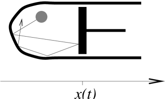
Figure 1: The prototype piston model. A gas particle is moving chaotically inside a cylinder. The driving is achieved by moving a wall element (”piston”).

The classic example for a driven system is the piston model (Fig.1), where a gas in confined inside a cylinder, and $x$ is the position of the piston. Our interest is in the case where we have ”one particle gas”. [Note however that if we know to solve the problem for one particle, then automatically we can get the solution for many non-interacting particles].

The 1D-box version of this model (Fig.2a) is known in the literature as the ”infinite-well” problem with moving wall infwell_a ; infwell_b . Some limited aspects of this problem have been discussed in the literature in connection with the Fermi acceleration problem jose .

A 2D-box variation of the ”piston model” is presented in Fig.2b. Here we have stadium shaped billiard, and the the parameter $x$ controls the deformation of the boundary. Two other variations of the same model are presented in Fig.3, where the box has the shape of a generalized Sinai billiard.

In the examples so far the parameter $x$ controls the shape of the ”box”, and $V=\dot{x}$ has the interpretation of wall velocity. The interest in such systems has emerged long time ago in studies of nuclear friction (one-body dissipation) wall ; koon . A renewed interest is anticipated in mesoscopic physics where the shape of a quantum dots can be controlled by gate voltages. [Note that in the nuclear physics context the shape is close to spherical, while a quantum dot is typically strongly chaotic].

We can create driving by changing any parameter (or field). In Fig.4 the driving is achieved by changing the perpendicular magnetic field. Fig.4a assumes ”quantum dot geometry” with homogeneous magnetic field, while Fig.4b assumes Aharonov-Bohm ring geometry with magnetic flux that goes via the hole. Let us define $x$ as the total magnetic flux. In such case $V=\dot{x}$ is the electro-motive force (measured in Volts) which is induced in the ring according to Faraday law.

If the variations of the parameter $x$ are classically small, then we can linearize the Hamiltonian as follows

$${\cal H}(Q,P;x)={\cal H}_{0}(Q,P)+x{\cal W}(Q,P)$$ (1)

where without loss of generality we have assumed that $x=0$ is the typical value of $x$. For generic systems (which means having smooth Hamiltonian that generates a classically chaotic motion), the representation of ${\cal W}$, in the ordered ${\cal H}_{0}$ determined basis, is known to be a banded matrix (for details see the next section). A simple example can be found in lds where

$${\cal H}(Q,P;x)=\mbox{\small$\frac{1}{2}$}(P_{1}^{2}{+}P_{2}^{2}+Q_{1}^{2}{+}Q_{2}^{2})+(1+x)\cdot Q_{1}^{2}Q_{2}^{2}$$ (2)

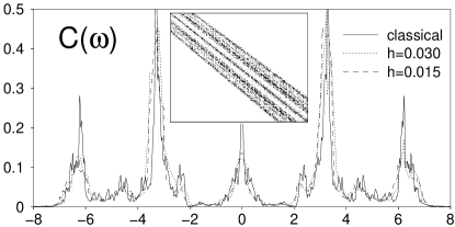
Figure 7: The band profile $(2\pi\hbar/\Delta)\cdot|{\mathbf{B}}_{nm}|^{2}$ versus $\omega=(E_{n}{-}E_{m})/\hbar$ is compared with $\tilde{C}(\omega)$. See text for further explanations. The calculation is done for the 2DW model of Eq.(2). The inset is an image of a piece of the ${\mathbf{B}}$ matrix. Taken from Ref.lds .

This Hamiltonian describes a particle moving inside a two dimensional anharmonic well (2DW). The shape of the 2DW in controlled by the parameter $x$. The perturbation is ${\cal W}(Q,P)=Q_{1}^{2}Q_{2}^{2}$, and its matrix representation ${\mathbf{B}}_{nm}$ is visualized in the inset of Fig.7.

The above discussion of generic Hamiltonian models, such as the 2DW model, motivates the definition of a simple artificial model Hamiltonian, that has the same characteristics: This is Wigner model wigner ; felix1 . In the following definition of Wigner model we follow closely the notations of wbr . In the standard representation ${\cal H}_{0}={\mathbf{E}}$ is a diagonal matrix whose elements are the ordered energies $\{E_{n}\}$, with mean level spacing $\Delta$, and ${\cal W}={\mathbf{B}}$ is a random banded matrix with non-vanishing couplings within the band $0<|n-m|\leq b$. These coupling elements are zero on the average, and they are characterized by the variance $\sigma=(\langle|{\mathbf{B}}_{nm}|^{2}\rangle)^{\mbox{\tiny 1/2}}$. Hence the Hamiltonian is

$${\cal H}={\mathbf{E}}+x{\mathbf{B}}$$ (3)

This artificial model can serve as a reference case for testing various theoretical ideas. Moreover, it has been conjectured that such model captures some generic features of chaotic systems. [Note that most of the RMT literature deals with simplified versions of Wigner model, where the bandwidth equals to the matrix size].

III Quantum Chaos

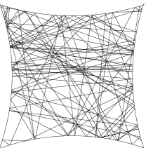
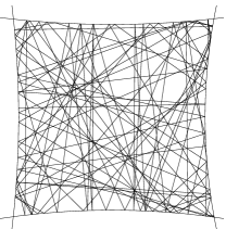
Figure 5: Chaotic trajectories inside a Sinai billiard. In both examples the motion is completely chaotic. This mean exponential sensitivity to any small change in the initial conditions. This sensitivity can be characterized by the ”Lyapunov exponent”. In the right illustration the motion is chaotic, but the chaos is weaker, which means smaller Lyapunov exponent.

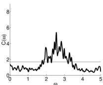
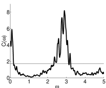
Figure 6: The power spectrum of the motion for the two examples of the previous figure. It is the power spectrum $\tilde{C}(\omega)$ of the fluctuating quantity ${\cal F}(t)=-d{\cal H}/dx$. The latter can be described as train of impulses (spikes) due to collisions with the walls. For strongly chaotic motion (left panel) the power spectrum of ${\cal F}(t)$ is like that of white noise. In the right panel the bouncing frequency is quite pronounced, and there is also a ”diabatic” peak around $\omega=0$. In both cases, the motion is characterized by a continuous power spectrum, which constitutes an indication for the chaotic nature of the motion.

The notion of chaos in classical mechanics implies that few degree of freedom system, such as the Sinai billiard system, exhibit stochastic-like behavior. This is in contrast to the out-of-date idea that stochasticity and irreversibility are the outcomes of having (infinitely) many degrees of freedom. Chaos means that the motion (eg Fig.5) has exponential sensitivity to any perturbation or change in initial conditions. Another way to characterize a chaotic motion is by its continuous power spectrum (see Fig.6). This should be contrasted with integrable motion which is characterized by a discrete (rather than continuous) set of frequencies.

For sake of later analysis it is useful to define the ”power spectrum” of the motion specifically as follows. Let $(Q(t),P(t))$ be an ergodic trajectory that is generated by the time independent Hamiltonian ${\cal H}(Q,P;x)$. We can define a fluctuating quantity ${\cal F}(t)=-d{\cal H}/dx$. In case that $x$ is the displacements of a wall element (eg Fig.3b), the fluctuating ${\cal F}(t)$ has the meaning of ”Newtonian force”. In case that $x$ is the magnetic flux (eg Fig.4b), the fluctuating ${\cal F}(t)$ has the meaning of ”electric current”. In case of the 2DW model we get ${\cal F}(t)=-{\cal W}(Q(t),P(t))=-Q_{1}(t)^{2}Q_{2}(t)^{2}$. The correlation function of the fluctuating ${\cal F}(t)$ will be denoted by $C(\tau)$ and the power spectrum of the fluctuations will be denoted by $\tilde{C}(\omega)$. The latter is the Fourier transform of the former. The variance of the fluctuation is $C(0)$, the intensity of the fluctuations is defined as $\tilde{C}(0)$, and the correlation time is denoted by $\tau_{cl}$.

It is clear that upon quantization we no longer have chaos. Still, the question arise what are the fingerprints of the classical chaos on both the spectral properties of the system, and also on the structure of the eigenstates. This problem was the focus of intensive studies during the last decade gutz ; haake ; sto , and it has important applications in mesoscopic physics imry ; alh_rev ; marcus_rev .

An important observation of ”quantum chaos” studies is that Quantum Mechanics introduce two additional energy scales into the problem (rather than only one). We can take the 2DW model as a generic example. After rescaling of the classical parameters of the model, we are left with one dimensionless parameter (the dimensionless energy). This parameter controls the nature of the classical dynamics. Upon quantization we have two additional (dimensionless) parameters. One energy scale is obviously the mean level spacing $\Delta$, which is proportional to $\hbar^{d}$. The other energy scale is $\Delta_{b}=\hbar/\tau_{cl}$, where $\tau_{cl}$ is the classical correlation time that characterizes the (chaotic) dynamics. If $\hbar$ is small then the two energy scales are very different ($\Delta\ll\Delta_{b}$).

The significance of the energy scale $\Delta_{b}$ is a central issue in ”quantum chaos”. It turns out that the statistical properties of the energy spectrum are universal on the sub-$\hbar$ scale, and obey the predictions of RMT. On the other hand, on large energy scale (compared with $\Delta_{b}$), non-universal (system specific) features manifest themselves berry . These features are the fingerprints of the underlying classical dynamics. In the context of ballistic quantum dots, which are in fact billiard systems, $\Delta_{b}$ is also know as the ”Thouless energy”.

There is another way in which the energy scale $\Delta_{b}$ manifests itself. Let ${\cal W}(Q,P)$ be some observable, and consider its matrix representation ${{\mathbf{B}}_{nm}}$ in the basis which is determined by the (chaotic) Hamiltonian. An example is presented in Fig.7. It can be argued mario that ${{\mathbf{B}}_{nm}}$ is a banded matrix, and that the bandwidth is $b=\Delta_{b}/\Delta$. This is based on a remarkably robust semiclassical expression that relates the bandprofile to the classical power spectrum:

$$\left\langle\left|{\mathbf{B}}_{nm}\right|^{2}\right\rangle\ \ \approx\ \ \frac{\Delta}{2\pi\hbar}\ \tilde{C}\left(\frac{E_{n}{-}E_{m}}{\hbar}\right)$$ (4)

We can apply this semiclassical relation to the case where ${\cal W}$ is the ”perturbation” as defined in Eq.(1). This leads to the interpretation of $\Delta_{b}$ as the largest ”distance” in energy space that can be realized in a first-order transition. We can also use the semiclassical relation in reverse, in order to find/define the classical correlation function that corresponds to a quantum-mechanical matrix Hamiltonian. In case of the standard Wigner model we get $C(\tau)=b\sigma^{2}\mbox{sin}(\tau/\tau_{cl})/(\tau/\tau_{cl})$, with the correlation time $\tau_{cl}=\hbar/(b\Delta)$.

IV Parametric Evolution

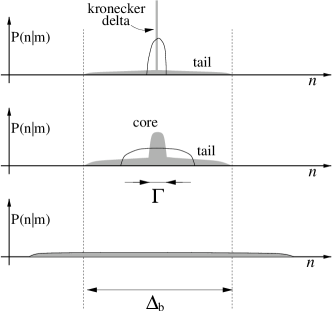
Figure 8: Upper panel: Schematic illustrations of the set of energies $E_{n}(x)$ which are obtained via diagonalization of a parameter dependent Hamiltonian. The thick solid line indicates the $n$-range where 50% of the $P(n|m)$ probability is concentrated ($m$ is fixed). The representative values $x_{1}$, $x_{2}$ and $x_{3}$ correspond to the standard perturbative regime, the core-tail (extended perturbative) regime, and the non-perturbative regime respectively. The corresponding LDOS structures are illustrated (grey shading) in the three plots of the lower panel. The semiclassical approximation (lines) is presented for sake of comparison.

A more recent development was to consider a parametric set of Hamiltonians, namely ${\cal H}(Q,P;x)$ where $x$ is a parameter as in the examples of Section 2. For each value of $x$ we can diagonalize the Hamiltonian, leading to set of (ordered) eigen-energies $E_{n}(x)$, as in the schematic illustration of Fig.8. The corresponding eigenstates will be denoted by $|n(x)\rangle$. Their parametric evolution can be characterized by the parametric kernel

$$P(n|m)=\left|\langle n(x)|m(x_{0})\rangle\right|^{2}$$ (5)

We shall use the notation $P(r)=P(n-m)=P(n|m)$, with implicit average over the reference state $m$. We shall refer to $P(r)$ as the ”average spreading profile”. This is in fact, up to scaling, the LDOS (local density of states, also known as strength function).

Let us characterize the perturbation by the quantity $\delta x=x-x_{0}$. The interesting question is how $P(r)$ evolves as we increase the perturbation $\delta x$. For the Wigner model the answer is known long ago wigner ; felix1 ; alh_brm ; rmt_rev . $P(r)$ has a standard perturbative structure for very small $\delta x$. For larger $\delta x$ it becomes a chopped Lorentzian, and for even larger $\delta x$ it becomes a semicircle. We shall denote the border between the standard perturbative regime and the Wigner regime by $\delta x_{c}$, and the border between the Wigner regime and the non perturbative (semicircle) regime will be denoted by $\delta x_{\mbox{\tiny prt}}$. The explicit expressions are:

$$\delta x_{c}\ =\ \frac{\Delta}{\sigma} \ \ \propto\ \ \hbar^{(1{+}d)/2}$$ (6)

$$\delta x_{\mbox{\tiny prt}}\ =\ \sqrt{b}\frac{\Delta}{\sigma} \ \ =\ \ \frac{2\pi\hbar}{\tau_{\mbox{\tiny cl}}\sqrt{C(0)}}$$ (7)

where $d$ is the number of freedoms ($d=2$ for billiards). In order to determine the $\hbar$ dependence we have used the semiclassical relation Eq.(4), and the proportionality $\Delta\propto\hbar^{d}$. Note that the latter relation, known as Wyle law, is significant for the determination of $\delta x_{c}$. In contrast to that $\delta x_{\mbox{\tiny prt}}\propto\hbar$ is in fact independent of $\Delta$.

The generalization of Wigner scenario has been the subject of our recent research wls ; lds ; prm . In the general case the standard perturbative structure evolves into a ”core-tail structure”, while for large $\delta x$ it becomes purely non-perturbative. In the standard perturbative regime ($\delta x\ll\delta x_{c}$) most of the probability $P(r)$ is concentrated in one level ($n=m$). In the extended perturbative regime most of the probability is concentrated within a ”core” whose width is typically $\Gamma(\delta x)\sim(\delta x/\delta x_{c})^{2}$. The ”core” is the non-perturbative component which arise due to non-perturbative mixing of nearby levels. The ”tail” is the outer perturbative component which is created by first order transitions.

The extended perturbative regime is defined by the requirement of having separation of energy scales $\Gamma(\delta x)\ll\Delta_{b}$. This condition is trivially satisfied in the ”standard perturbative regime” where $\Gamma\sim\Delta$. The condition $\Gamma(\delta x)\ll\Delta_{b}$ is violated in the non-perturbative regime ($\delta x\gg\delta x_{\mbox{\tiny prt}}$), which in fact leads to the determination of $\delta x_{\mbox{\tiny prt}}$ as in Eq.(7). The theory for $P(r)$ in the non-perturbative regime is not complete yet. However, it can be argued wls that if $\delta x$ is large enough, then $P(r)$ becomes of semiclassical nature felix2 . The case of billiards with shape deformation requires special considerations and is of particular interest wls ; prm .

It is important to realize that the border of the standard perturbative regime ($\delta x_{c}$) is related to the energy scale $\Delta$, while the border of the extended perturbative regime ($\delta x_{\mbox{\tiny prt}}$), which leads to the identification of the non-perturbative regime, is related to the bandwidth $\Delta_{b}$.

V Temporal evolution

After considering the parametric evolution, the next logical stage is to consider the actual (temporal) evolution which is generated by the time dependent Hamiltonian ${\cal H}(Q,P,x(t))$. Then, in complete analogy, we can ask how the energy scales $\Delta$ and $\Delta_{b}$ are reflected in the actual evolution. We postpone the discussion of the latter issue to Section 11.

The purpose of the present and next sections is to define what does it mean ”driving”, and how do we quantify the temporal evolution. Without loss of generality we assume $x(0)=0$. We would like to consider the following driving schemes:

• Linear driving

• One pulse driving cycle

• Periodic driving

• Driving reversal scenario

• Time reversal scenario

In the next section we define the various schemes, some of which are also illustrated in Fig.9. The evolution is characterized by the obvious generalization of Eq.(5), namely

$$P_{t}(n|m)=\left|\langle n(x(t))|U|m(x(0))\rangle\right|^{2}$$ (8)

Here $U$ is the evolution operator, with implicit dependence on the time $t$. The parametric kernel Eq.(5) can be regarded as corresponding to the ”sudden” limit where $U\approx 1$. As in the parametric case we can define an average spreading profile $P_{t}(r)$, where $r=n-m$.

There are various practical possibilities available for the characterization of the distribution $P_{t}(r)$. It turns out that the major features of this distribution are captured by the following three measures:

$${\cal P}(t) = P_{t}(r=0)$$ (9)

$$\Gamma(t) =$$ 50% probability width (10)

$$\delta E(t) = \Delta\times\left(\sum_{r}r^{2}P_{t}(r)\right)^{1/2}$$ (11)

The first measure is the survival probability ${\cal P}(t)$. The second measure $\Gamma(t)$ is the energy width of the central $r$ region that contains 50% of the probability. [For simplicity of presentation we use here a loose definition of $\Gamma$ as far as prefactors of order unity are concerned.] Finally the energy spreading $\delta E(t)$ is defined as the square-root of the variance.

It is important to realize that the above three measures give different type of information about the nature of the energy spreading profile. In particular the indication for having a core-tail structure is:

$$\Gamma(t)\ \ \ll\ \ \delta E(t)\ \ \ll\ \ \Delta_{b}$$ (12)

The core-tail structure (eg chopped Lorentzian) is characterized by a ”tail” component that contains a vanishingly small probability but still dominates the variance. [Note that $\Delta_{b}=\infty$, as in the case of un-chopped Lorentzian, would imply $\delta E(t)=\infty$ irrespective of $\Gamma$.] In contrast to that a typical semiclassical spreading profile (as well as Wigner’s Semicircle) is characterized by

$$\delta E(t)\ \ \sim\ \ \Gamma(t)\ \ \gg\ \ \Delta_{b}$$ (13)

In the latter case, in order to avoid confusion, it is better not to use the notation $\Gamma(t)$. [The notation $\Gamma$ has been adopted in the common diagrammatic formulation of perturbation theory. This formulation is useful in the extended perturbative regime in order to derive Wigner’s chopped Lorentzian. In the non-perturbative regime this formulation becomes useless, and therefore the significance of $\Gamma$ is lost.]

VI Driving schemes

Linear driving means $x(t)=Vt$, where $V$ is a constant. In such a scenario obviously $x(t)\neq x(0)$. Still it is convenient to assume that the chaotic nature of the dynamics is independent of $x$, and that changes in $x$ are not associated with changes in phase space volume (no conservative work is being done). This is manifestly the case for the systems which are illustrated in Fig.3b and Fig.4b. [Note that the standard Wigner model does not have $x$ invariance property, and therefore the analysis of linear driving for the Wigner model is an ill defined problem. Attempts to overcome this difficulty lead to certain subtleties rsp ].

For all the other driving schemes we assume, without loss of generality, that $x(0)=x(T)=0$, where $T$ is the period of the driving cycle. The simplest driving scheme is a rectangular pulse $x(0<t<T)=A$, which is characterized by its amplitude $A$. Does the study of rectangular pulses constitute a good bridge for developing a general theory for driven systems? The answer is definitely not. An essential ingredient in the theory of driven system is the rate $V$ in which the parameter $x$ is being changed in time. Therefore, it is important to consider, for example, a triangular pulse (Fig.9b). Such pulse is characterized by both amplitude $A$ and driving rate $V=2A/T$. More generally one may consider (Fig.9c) a train of such pulses ($=$ periodic driving). In particular one may consider the usual sinusoidal driving $x(t)=A\sin(\Omega t)$ where $\Omega=2\pi/T$. In the later case we can define the root-mean-square driving rate as $V=\Omega A/\sqrt{2}$.

In all these cases we ask, in complete analogy with the parametric case, what is the evolution of the energy distribution $P_{t}(r)$. Now the evolution is with respect to time, rather than with respect to $\delta x$. The different scenarios are distinguished by the choice of $U$. We shall use the notation $U[x_{A}]$ in order to denote the evolution operator that corresponds to driving scheme $x=x_{A}(t)$.

The case of rectangular pulse is known in the literature as ”wavepacket dynamics” heller . The particle is prepared in an eigenstate of the ${\cal H}_{0}$ Hamiltonian, while the evolution is generated by the perturbed Hamiltonian ${\cal H}={\cal H}(Q,P;x=A)$. We may consider more complicated schemes of pulses. For example rectangular pulse $+A$ followed by another rectangular pulse $-A$. The question here is whether the second pulse can compensate the effect of the first pulse. We call such scheme ”driving reversal”. The evolution operator can be written as $U=U[x(\mbox{\small rev})]U[x]$ where $x=A$ represents the rectangular pulse, while $x(\mbox{\small rev})=-A$ is the reversed pulse. The case of triangular pulse can be regarded as another particular variation of driving reversal. In the latter case $x$ represents linear driving with velocity $V$, and $x(\mbox{\small rev})$ is the reversed driving process with velocity $-V$.

The case of ”driving reversal” should be distinguished from ”time reversal” scheme. The latter notion is explained in the next section.

VII Two notions of irreversibility

There are two distinct notions of irreversibility in statistical and quantum mechanics. One is based on the ”piston model” paradigm (PMP), while the other peres is based on the ”ice cube in cup of hot water” paradigm (ICP). The recent interest jalabert ; jacq ; tomsovic ; fdl ; prosen ; rvs in ”quantum irreversibility” is motivated by its relevance to quantum computing.

In the PMP case we say that a process is reversible if it is possible to ”undo” it by driving reversal. Consider a gas inside a cylinder with a piston (Fig.1). Let us shift the piston inside. Due to the compression the gas is heated up. Can we undo the ”heating” simply by shifting the piston outside, back to its original position? If the answer is yes, as in the case of strictly adiabatic process, then we say that the process is reversible.

In the ICP case we consider the melting process of an ice cube. Let us assume that after some time we reverse the velocities of all the molecules. If the external conditions are kept strictly the same, we expect the ice-cube to re-emerge out of the water. In practice the external conditions (fields) are not exactly the same, and as a result we have what looks like irreversibility.

The mathematical object that should be considered in order to study PMP is just $P_{t}(r)$ for a driving scheme that involves ”driving reversal”. Namely, as discussed in the previous section, the evolution operator is

$$U\ \ =\ \ U[x(\mbox{\small rev})]\ U[x]$$ (14)

The mathematical object that should be considered in order to study ICP is again $P_{t}(r)$, but with driving scheme that involves ”time reversal”. Namely, the evolution operator is defined as

$$U\ \ =\ \ U[x_{B}]^{-1}\ U[x_{A}]$$ (15)

In the latter case, if the external conditions are in full control ($x_{B}=x_{A}$), then we have complete reversibility ($U=1$).

It is also important to define precisely what is the measure for quantum irreversibility. This is related to the various possibilities which are available for the characterization of the distribution $P_{t}(r)$. The prevailing possibility is to take the survival probability ${\cal P}(t)$ as a measure peres . Another possibility is to take the energy spreading $\delta E(t)$ as a measure. The latter definition goes well with the PMP, and it has a well defined classical limit. Irreversibility in this latter sense implies diffusion in energy space, which is the reason for having energy absorption (dissipation) in driven mesoscopic systems (see section 9).

VIII Wavepacket dynamics, survival probability and fidelity

Driving schemes with rectangular pulses are the simplest for both analytical and numerical studies. It is easiest to consider the survival probability in case of a single rectangular pulse. The survival amplitude is defined as

$$F(t) = \langle\Psi_{0}|U[A]|\Psi_{0}\rangle$$ (16)

$$= \left|\left\langle\Psi_{0}\Big{|}\exp\left(-\frac{i}{\hbar}{\cal H}t\right)\Big{|}\Psi_{0}\right\rangle\right|$$

The survival probability is ${\cal P}(t)=|F(t)|^{2}$, in consistency with the definition of Eq.(9). $F(t)$ is manifestly a Fourier transform of the LDOS, and therefore we can immediately draw a conclusion wls that the nature of the dynamics is different depending on the parametric regime to which the amplitude $A$ belongs. If $P(r)$ have a core-tail Lorentzian structure, then we get an exponential decay ${\cal P}(t)=\exp(-\Gamma t)$. On the other hand if $P(r)$ has a semiclassical structure, then the decay of ${\cal P}(t)$ is non-universal (system specific).

A similar picture arise in recent studies of the survival probability for ”time reversal” driving scheme. Here one defines the fidelity amplitude as

$$F(t)=\langle\Psi_{0}|U[A]^{-1}U[0]|\Psi_{0}\rangle$$ (17)

The fidelity, also known as Loschmidt echo, is defined as ${\cal P}(t)=|F(t)|^{2}$. The situation here is more complicated compared with Eq.(16) because we have two LDOS functions fdl : one is the ${\cal H}_{0}$ weighted LDOS, and the other is the $\Psi_{0}$ weighted LDOS. The two LDOS functions coincide only if $\Psi_{0}$ is an eigenstate of ${\cal H}_{0}$. In the latter case the $F(t)$ of Eq.(17) reduces (up to phase factor) to Eq.(16). It turns out that in case of Eq.(17) there is no simple Fourier Transform relation between $F(t)$ and the LDOS functions. However, the picture ”in large” is the same as in the case of Eq.(16) fdl . Namely, one has to distinguish between three regimes of behavior: In the standard perturbative regime ($A<\delta x_{c}$) one typically encounters a Gaussian decay peres ; In the Wigner regime (also called FGR regime) one typically finds Exponential decay jacq ; And in the non-perturbative regime one observes a semiclassical perturbation-independent ”Lyapunov decay” jalabert .

The study of the survival probability, as described above, is only one limited aspect of the temporal evolution. The more general object that should be considered is $P_{t}(r)$ as defined in section 5. The major features of this time evolution are captured by the three measures that we have defined in Eq.(9)-(11). In Fig.10 we display numerical simulations of wavepacket dynamics for the 2DW model. The energy spreading $\delta E(t)$ is plotted as a function of time. The first panel is the classical simulation, which in fact coincides with the ”linear response” calculation. The input for the LRT calculation is $C(\tau)$, and the result is proportional to the amplitude $A$. Namely,

$$\delta E(t)=A\times\sqrt{2(C(0)-C(t))}$$ (18)

In the second panel we display the results of the quantum mechanical simulations. For smaller $\hbar$ values the agreement with the classical LRT calculation is better. Finally, in the third panel we repeat the quantum mechanical simulations with a sign randomized Hamiltonian. This means that we take Eq.(3), and we randomize the sign of the off-diagonal terms. The bandprofile, and hence $\tilde{C}(\omega)$ are not affected by this procedure, which implies that the LRT calculation gives exactly the same result. But now we see that as $\hbar$ becomes smaller the correspondence with the classical result becomes worse. Specifically: In (a) and (b) we see a crossover from ballistic spreading ($\delta E\propto t$) to saturation ($\delta E\sim\mbox{const}$) as implied by Eq.(18). Only one time scale ($\tau_{\mbox{\tiny cl}}\sim 1$) is involved. In (c), in contrast to that, we see that as $\hbar\rightarrow 0$ an intermediate stage of diffusion ($\delta E\propto\sqrt{t}$) develops.

How can we explain the above results. Obviously we see that for small $\hbar$ we cannot trust LRT. What in fact happens is that we have a crossover from the perturbative regime ($A<\delta x_{\mbox{\tiny prt}}(\hbar)$) to the non-perturbative regime ($A>\delta x_{\mbox{\tiny prt}}(\hbar)$). In the latter case we get either semiclassical behavior, or RMT behavior. In other words, random matrix theory and the semiclassical theory lead to different non-perturbative limits. In the semiclassical case the crossover from LRT behavior to non-perturbative behavior cannot be detected by looking on $\delta E(t)$. Still the crossover can be detected by looking on $\Gamma(t)$. See wpk for details.

IX Diffusion in energy space and Dissipation

In the following sections we discuss the case of either linear or periodic driving. In such case the long time behavior of the system is characterized by diffusion in energy space. Associated with this diffusion is a systematic increase of the average energy. This irreversible process of energy absorption is known as ”dissipation”.

There is a satisfactory classical theory for dissipation cl_dsp . Some of the mathematical details are subtle, but the overall physical picture is quite simple. Without loss of generality the main idea can be explained by referring to the billiard example of Fig.1a. The particle executes chaotic motion, and we may say that each collision has roughly equal probability to be with either the inward-going or with the outward-going wall. As a result the particle either gain or loose kinetic energy. Thus, the dynamics in energy space is like random walk, and it can be described by a diffusion equation. Thus we see that due to the chaos we have stochastic-like energy spreading.

This classical diffusion process is irreversible in the PMP sense. Let us assume that we start with a microcanonical distribution that has definite energy. If, after some time, we reverse the velocity of the walls, then obviously we do not get back the initial microcanonical distribution.

The effect of dissipation is related to the irreversible stochastic-like diffusion in energy space. If the diffusion rate were the same irrespective of the energy, then obviously the average energy would be constant. But this is not the case. The diffusion is stronger as we go up in energy, and as a result the diffusion process is biased. Thus the average energy systematically grows with time, and one can derive a general diffusion dissipation relation flc :

$$\frac{d}{dt}\langle{\cal H}\rangle\ =\ -\int_{0}^{\infty}dE\ g(E)\ D_{\mbox{\tiny E}}\ \frac{\partial}{\partial E}\left(\frac{\rho(E)}{g(E)}\right)$$ (19)

where $g(E)$ is the density of states, and $\rho(E)$ is the probability distribution (eg microcanonical, canonical or Fermi occupation). The diffusion picture is generally valid in the classical case, and it is typically valid also in the quantum mechanical case. [The issue of dynamical localization due to strictly periodic driving qkr is important for driven 1D system, but not so important in the case of driven chaotic systems rsp .]

There is a simple linear response (Kubo) expression, that relates the diffusion coefficient to the power spectrum $\tilde{C}(\omega)$ of the fluctuations:

$$D_{\mbox{\tiny E}}\ \ =\ \ \frac{1}{2}\tilde{C}(\Omega)\times V^{2}$$ (20)

The diffusion law for short times is $\delta E(t)=\sqrt{2D_{\mbox{\tiny E}}t}$. This expression is completely analogous to Eq.(18). In both cases the spreading is proportional to the amplitude $A$. [Recall that for periodic driving we define $V=\Omega A/\sqrt{2}$. In the special case of linear driving the spreading is proportional to $V$.] Moreover, as in the case of wavepacket dynamics, the LRT result is the same classically and quantum-mechanically. But again, as in the case of the wavepacket dynamics, the validity regime of LRT in the quantum mechanical case is much smaller (see section.11).

If we combine the above Kubo expression with the diffusion-dissipation relation we get

$$\frac{d}{dt}\langle{\cal H}\rangle=\mu(\Omega)\times V^{2}$$ (21)

where $\mu$ is related to the power spectrum of the fluctuations. Thus we get a fluctuations-dissipation relation flc . The standard ”thermal” fluctuation-dissipation relation $\mu(0)=\tilde{C}(0)/(2k_{B}T)$ is obtained from Eq.(19) in case of canonical $\rho(E)$.

Standard textbook formulations flc takes linear response theory together with thermal statistical assumptions as a package deal. Our presentation provides a more powerful picture. On the one hand we can discuss non-equilibrium situation using LRT combined with an appropriate version of the diffusion-dissipation relation. On the other hand, we may consider situation where LRT does not apply. In such case we may get some (non-perturbative) result for the diffusion, and later use the diffusion-dissipation relation in order to calculate the dissipation rate.

X Beyond kinetic theory

The coefficient $\mu$ in Eq.(21) is called the ”dissipation coefficient”. In the case where $x$ is the displacement of a wall element, it is also known as ”friction coefficient”, and in the case where $x$ is a magnetic flux it can be called ”conductance”.

Having dissipation rate proportional to $V^{2}$ is known as ”ohmic” behavior. In case of ”friction” it is just equivalent to saying that there is a friction force proportional to the velocity $V$, against which the wall is doing mechanical work. This mechanical work is ”dissipated” and the gas is ”heated up” in a rate proportional to $V^{2}$.

In case of ”conductance” we may say that there is a drift current proportional to the voltage $V$. This is in fact ”Ohm law”. The dissipated energy can either be accumulated by the electrons (as kinetic energy), or it may be eventually transfered to the lattice vibrations (phonons). In the latter case we say that the ring is ”heated up”. The rate of the heating goes like $V^{2}$ which is in fact ”Joule law”.

The traditional approach to calculate $\mu$ is to use a kinetic picture (Boltzmann) which is based on statistical assumptions. This leads in case of friction to the ”wall formula” wall ; koon :

$$\mu(\Omega)=\frac{N}{\mathsf{V}_{\mbox{\tiny box}}}mv_{\mbox{\tiny E}}\mathsf{A}_{\mbox{\tiny walls}}$$ (22)

where $N$ is the number of gas particles (let us say $N=1$), and $v_{\mbox{\tiny E}}=\sqrt{2E/m}$. We also use the notations ${\mathsf{V}_{\mbox{\tiny box}}}$ for the volume of the box, and $\mathsf{A}_{\mbox{\tiny walls}}$ for the effective area of the moving walls. In the latter we absorb some geometric factors frc . Application of the traditional kinetic (Boltzmann) approach in case of conductance leads to ”Drude formula”:

$$\mu(\Omega)\ \sim\ \frac{N}{{\mathsf{A}}_{\mbox{\tiny dot}}}\left(\frac{e^{2}}{m}\tau_{\mbox{\tiny col}}\right)\frac{1}{1+(\tau_{\mbox{\tiny col}}\Omega)^{2}}$$ (23)

where ${\mathsf{A}}_{\mbox{\tiny dot}}$ is the area of the ”quantum dot”, and $\tau_{\mbox{\tiny col}}$ is the average time between collisions with the walls.

Using Linear response theory (Kubo formula), as described in the previous section, we can go beyond the over-simplified picture of kinetic theory. That means to go beyond Boltzmann picture. Below we explain under what assumptions we get the ”traditional” kinetic expressions, and what in fact can go wrong with these assumptions.

The interest in friction calculation has started in studies of ”one body dissipation” in nuclear physics wall ; koon . The ”wall formula” assumes that the collisions are totally uncorrelated. In such case the power spectrum $\tilde{C}(\omega)$ of ${\cal F}(t)$ is like that of white noise (namely ”flat”). By inspection of Fig.6 we can see that this assumption is apparently reasonable in the limit of very strong chaos. But it is definitely a bad approximation in case of weak chaos. The dynamics of chaotic system is typically characterized by some dominant frequencies. Therefore we have relatively strong response whenever the driving frequency matches a ”natural” frequency of the system. This can be regarded as a classical (broad) resonance. By inspection of Fig.6 we see that a particular feature is having such resonance around $\omega=0$. This type of resonance, due to bouncing behavior, can be regarded as a ”classical diabatic effect” dia .

Even if the chaos is very strong, the ”white noise” assumption is not necessarily correct: In dil ; wlf we explain that for special class of deformations (including translations, rotations and dilations) the low frequency response is suppressed, irrespective of the chaoticity. This is illustrated numerically in Fig.11.

In case of Drude formula the fluctuating ${\cal F}(t)$ has the meaning of ”electric current”, and therefore the power spectrum $\tilde{C}(\omega)$ is the Fourier transform of the current-current (or one may say velocity-velocity) correlation function. Assuming that the velocity-velocity correlation function decays exponentially in time, one obtains the Drude result. A careful analysis of this assumption, and its relation to the ”white noise approximation” of the ”wall formula”, can be found in Section 6 of wlf . Fig.12 displays a numerical example. We clearly see non-universal deviations from the Drude expression, which reflect the specific geometry of the ”quantum dot”.

XI Non-perturbative response

In the classical case, assuming idealized system, the crossover to stochastic energy spreading involves only one time scale, which is $\tau_{\mbox{\tiny cl}}$. Gaussian-like spreading profile is obtained only for time $t$ much larger than $\tau_{\mbox{\tiny cl}}$. For short times we can use linear analysis in order to calculate the spreading profile. However, this analysis has a breaktime frc that we call $t_{\mbox{\tiny frc}}(V)$, where $V$ is the rate in which $x$ is being changed. For long times ($t\gg\tau_{\mbox{\tiny cl}}$) we can use stochastic picture. Classical LRT calculation of the diffusion is valid only if the crossover to stochastic behavior is captured by the short time analysis. This leads to the classical slowness condition $\tau_{\mbox{\tiny cl}}\ll t_{\mbox{\tiny frc}}(V)$ which we assume from now on. See specific examples in Sections 13 and 14.

In the quantum mechanical case we follow a similar reasoning. The linear analysis is carried out using perturbation theory. We have presented frc a careful analysis to determine the breaktime $t_{\mbox{\tiny prt}}(V;\hbar)$ of this analysis. It turns out that this breaktime is not related to the mean level spacing $\Delta$, but rather to the much larger energy scale $\Delta_{b}$.

In complete analogy with the classical analysis, it turns out that the validity of LRT in the quantum domain is restricted by the condition $\tau_{\mbox{\tiny cl}}\ll t_{\mbox{\tiny prt}}(V;\hbar)$. If this inequality is not satisfied, then we say that we are in a non-perturbative regime. It is important to realize that the $\hbar\rightarrow 0$ limit is a non-perturbative limit. This means that the semiclassical regime is contained within the non-perturbative regime.

In the simple examples that are discussed in Sections 13 and 14, the non-perturbative regime is in fact a semiclassical regime. This coincidence does not hold in general vrn ; crs ; frc . In case of RMT models, obviosly we do not have a semiclassical limit. In such models the non-perturbative response deviates significantly from Kubo formula (Fig.13). The interest in such models can be physically motivated by considering transport in quantized disordered systems. Whether similar deviations from Kubo formula can be found in case of quantized chaotic systems is still an open question rsp . In any case, it is important to remember that the rate of dissipation is just one aspect of the energy spreading process. Even if Kubo formula does not fail (thanks to quantum-classical correspondence), still there are other features of the dynamics that are affected by the crossover from the perturbative to the non-perturbative regime. For example: in Sec.19 we are going to show that different results are obtained for the dephasing time, depending whether the process is perturbative or non-perturbative.

We can express the condition for being in the non-perturbative regime as frc

$$V\ \ \gg\ \ \frac{\delta x_{\mbox{\tiny prt}}}{\tau_{cl}}$$ (24)

The expression in the right hand side scales like $\hbar$, which reflects that this condition is related to $\Delta_{b}$ and not to $\Delta$. In the next section we discuss the definition of the adiabatic regime (very small $V$) whose existence is related to having finite $\Delta$. A schematic illustration of the three regimes (adiabatic, LRT, non-perturbative) is presented in Fig.14. Some further reasoning rsp allows to define the non perturbative regime in case of periodic driving. Its location in $(A,\Omega)$ space is also illustrated in Fig.14. Note that for periodic driving we define $V=\Omega A/\sqrt{2}$. The two $V=\mbox{const}$ curves in the $(\Omega,A)$ diagram represent the same conditions as in the case of linear driving. Other details of this diagram are discussed in the next section, and in rsp .

XII Adiabatic response and QM resonances

Let us assume that we are in the perturbative regime (which means that the non-perturbative regime of the previous section is excluded). We ask the following question: can we use the classical Kubo result as an approximation for the quantum mechanical result? The answer is ”yes” with the following restrictions: (i) The amplitude of the driving should be large enough; (ii) The frequency of the driving should be large enough. The two conditions are further discussed below. If they are satisfied we can trust the classical result. This follows from the remarkable quantal-classical correspondence which is expressed by Eq.(4). We have an illustration of this remarkable correspondence in Figures 7 and 11.

Large enough amplitude means $A\gg\delta x_{c}$. One may say that large-amplitude driving leads to effective ”broadening” of the discrete levels, and hence one can treat them as if they form a continuum. This is essential in order to justify the use of Fermi golden rule (FGR) for a small isolated system rsp . Kubo formula can be regarded as a consequence of FGR. If the driving amplitude is not large enough to ”mix” levels, we cannot use FGR, but we can still use first order perturbation theory as a starting point. Then we find out, as in atomic physics applications, that the response of the system is vanishingly small unless the driving frequency $\omega$ matches energy level spacing. This is called ”QM resonance”. The strips of QM resonances are illustrated in the schematic diagram of Fig.14. It is important to realize that higher order of perturbation theory, and possibly non-perturbative corrections, are essential in order to calculated the non-linear response in this regime wilk . Still, first order perturbation theory is a valid starting point, and therefore we do not regard this (non-linear) regime as ”non-perturbative”.

Large enough frequency means $\omega\gg\Delta/\hbar$. The remarkable quantal-classical correspondence which is expressed by Eq.(4) is valid only on energy scales that are large compared with $\Delta$. If this condition is not satisfied, we have to take into account the level spacing statistics robbins ; ophir . This means that we can have significant difference between the quantal LRT calculation, and the classical LRT calculation.

However, this is not the whole story. If $V$ is small enough, first order perturbation theory implies ”QM adiabaticity”. The condition for QM adiabaticity is $V\ll\delta x_{c}/t_{\mbox{\tiny H}}$ where $t_{\mbox{\tiny H}}=2\pi\hbar/\Delta$ is the Heisenberg time. A useful way of writing the QM adiabaticity conditions is:

$$V\ \ \ll\ \ \frac{1}{b^{3/2}}\left(\frac{\delta x_{\mbox{\tiny prt}}}{\tau_{cl}}\right)$$ (25)

In the adiabatic regime, first order perturbation theory implies zero probability to make a transition to other levels. Therefore, to the extend that we can trust the adiabatic approximation, all the probability remains concentrated in the initial level. Thus, in this regime, as in the case of small amplitudes, it is essential to use higher orders of perturbation theory, and non-perturbative corrections (Landau-Zener wilk ). Still we emphasize that first order perturbation theory is in fact a valid starting point, and therefore we do not regard this (non-linear) regime as ”non-perturbative”.

XIII Driving by electro-motive force

Consider a charged particle moving inside a chaotic ring. Let $x$ represent a magnetic flux via the ring. If we change $x$ in time, then by Faraday law $V=\dot{x}$ is the electro-motive force (measured in Volts). The fluctuating quantity ${\cal F}(t)$ has the meaning of electric current. The variance of the fluctuations is $C(0)=(ev_{\mbox{\tiny E}}/L)^{2}$, where $v_{\mbox{\tiny E}}=\sqrt{2E/m}$, and $L$ is the length of the ring. The correlation time of these fluctuations is the ballistic time $\tau_{cl}=\tau_{\mbox{\tiny col}}=L_{\mbox{\tiny col}}/v_{\mbox{\tiny E}}$.

Having characterized the fluctuations, we can determine the bandwidth $\Delta_{b}=\hbar/\tau_{\mbox{\tiny col}}$. A straightforward calculation leads to the result:

$$b\ \ =\ \ \left[\frac{L}{L_{\mbox{\tiny col}}}\right]\times\left(\frac{L_{\perp}}{\lambda_{\mbox{\tiny E}}}\right)^{d{-}1}$$ (26)

where $\lambda_{\mbox{\tiny E}}=2\pi\hbar/(mv_{\mbox{\tiny E}})$ is the De-Broglie wavelength, and $L_{\perp}$ is the width of the ring. Using Eq.(7) we can determine the non-perturbative parametric scale:

$$\delta x_{\mbox{\tiny prt}}\ \ =\ \ \left[\frac{L}{L_{\mbox{\tiny col}}}\right]\times\frac{\hbar}{e}$$ (27)

which up to a geometric factor equals the quantal flux unit. Note that in order to mix levels a relatively small change in the flux is needed, as implied by comparing Eq.(6) with Eq.(7).

We turn now to the analysis of the spreading in the time dependent case, say for linear driving. The classical ”slowness” condition which has been mentioned in section 11 is simply $eV\ll E$ where $E$ is the kinetic energy of the charged particle. Upon quantization we should distinguish the non-perturbative regime using Eq.(24), leading to

$$eV\ \ \gg\ \ \left[\frac{L}{L_{\mbox{\tiny col}}}\right]\frac{\hbar}{\tau_{\mbox{\tiny col}}}$$ (28)

Disregarding the geometric prefactor, the quantity in the right hand side is the so called Thouless energy. We also should distinguish the QM adiabatic regime using Eq.(25), leading to

$$eV\ \ \ll\ \ \left(\frac{\lambda_{\mbox{\tiny E}}}{L}\right)^{3/2}\frac{\hbar}{\tau_{\mbox{\tiny col}}}$$ (29)

where we have assumed for simplicity a simple 2D quantum dot geometry as in Fig.4a.

XIV Driving by moving walls

There is an ongoing interest infwell_a ; infwell_b in the problem of 1D box with moving wall (also known as the infinite well problem with moving wall). If the wall is moving with constant velocity, then it is possible to transform the Schrodinger equation into a time-independent equation, and to look for the stationary states.

We are interested in the dynamics, and therefore we would like to go beyond this limited scope of study. Before we discuss the general case, it is useful to point out the $d>1$ generalization of the above picture. We can easily show that for any ”special deformation” which is executed in either constant ”velocity” or ”acceleration”, we can transform the Schrodinger equation into a time-dependent equation. By ”special deformation” we mean either translation or rotation or dilation, or any linear combination of these. The statement is manifestly trivial for translations and rotations (it is like going to a different reference frame), but it is also true for dilations. The 1D box with moving wall is just a special case of dilation.

It is important to realize that in case of generic deformation of chaotic box, we cannot ”eliminate” the time dependence. Thus it is not possible to reduce the study of ”dynamics” to a search for ”stationary solutions”.

The determination of $\Delta_{b}$ for this system is quite obvious but subtle prm . As one can expect naively the result is $\Delta_{b}=2\pi\hbar/\tau_{\mbox{\tiny col}}$, where $\tau_{col}$ is the mean time between collisions with the moving walls. The subtlety here is that we cannot interpret $\Delta_{b}$ as ”bandwidth”. Formally the correlation time of ${\cal F}(t)$ is $\tau_{cl}=\infty$ which implies infinite bandwidth. Still, some non-trivial reasoning wls ; prm leads to the conclusion that the naive result (rather than the ”formal” one) is in fact effectively correct. A straightforward calculation leads to the result:

$$b\ \ =\ \ \frac{{\mathsf{V}}_{\mbox{\tiny box}}}{L_{\mbox{\tiny col}}\lambda_{\mbox{\tiny E}}^{d{-}1}}\ \ =\ \ \frac{{\mathsf{A}}_{\mbox{\tiny walls}}}{\lambda_{\mbox{\tiny E}}^{d{-}1}}$$ (30)

where $\lambda_{\mbox{\tiny E}}=2\pi\hbar/(mv_{\mbox{\tiny E}})$ is the De-Broglie wavelength, and ${\mathsf{V}}_{\mbox{\tiny box}}$ is the volume of the box, and $L_{\mbox{\tiny col}}$ is the mean free path between collisions. As for the effective value of $\delta x_{\mbox{\tiny prt}}$, again the details are subtle, but the naive guess turns out to be correct. With the proper (natural) choice of units for the displacement parameter $x$, the result is simply $\delta x_{\mbox{\tiny prt}}=\lambda_{\mbox{\tiny E}}$.

The way to analyze the dynamics for box with moving walls is outlined in wld . The classical LRT domain is $V\ll v_{\mbox{\tiny E}}$, where $v_{\mbox{\tiny E}}=\sqrt{2E/m}$. Upon quantization we should distinguish the non-perturbative regime using Eq.(24), leading to

$$V\ \ \gg\ \ \frac{\hbar}{mL_{\mbox{\tiny col}}}$$ (31)

In the non-perturbative regime the dynamics has a semiclassical nature, and the energy spreading process has a resonant random-walk nature. This should be contrasted with the behavior in the perturbative non-adiabatic regime, where Fermi-golden-rule (FGR) picture applies.

We also should distinguish the QM adiabatic regime using Eq.(25), leading to

$$V\ \ \ll\ \ \left(\frac{\lambda_{\mbox{\tiny E}}^{d{-}1}}{{\mathsf{A}}_{\mbox{\tiny walls}}}\right)^{3/2}\frac{\hbar}{mL_{\mbox{\tiny col}}}$$ (32)

In the QM adiabatic regime the spreading is dominated by transitions between near-neighbor levels: This is the so called Landau-Zener spreading mechanism wilk . See also Section 20 of frc , and the numerically related work in diego .

XV Brownian motion

Brownian motion is a paradigm for the general problem of system that interacts with its environment. (See Fig.15 and general discussion in the next section). One can imagine, in principle, a ”zoo” of models that describe the interaction of a Brownian particle with its environment. However, following Caldeira and Leggett zcl , the guiding philosophy is to consider ”ohmic models” that give Brownian motion that is described by the standard Langevin equation in the classical limit. Four families of models are of particular interest:

• Interaction with chaos.

• Interaction with many-body bath.

• Interaction with harmonic bath.

• Interaction with random-matrix bath.

Below we assume that the total Hamiltonian has the following general form

$${\cal H}_{\mbox{\tiny total}}\ =\ {\cal H}_{0}(x,p)\ +\ {\cal H}(Q,P;x)$$ (33)

where $(x,p)$ are the system coordinates, and $(Q,P)$ are the environmental degrees of freedom.

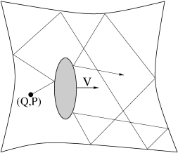
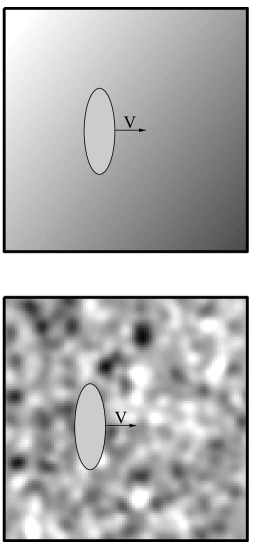
Figure 16: (a) The Brownian motion is induced due to the interaction with chaotic degrees of freedom. (b) The Brownian particle in the ZCL model experiences a fluctuating homogeneous field of force. (c) In case of the DLD model the fluctuating field is farther characterized by a finite correlation distance. In (b) and (c) the background image is a ”snapshot” of the fluctuating environment. Namely, the gray levels correspond to the ”height” of an instantaneous potential which is experienced by the Brownian particle.

Interaction with chaos provides the simplest model for Brownian motion jar . See Fig.16a for illustration of the model. The large Brownian particle is described by the canonical coordinates $(x,p)$, while the gas particles are described by the canonical coordinates $(Q,P)$. It is important to realize that in order to have Brownian motion, it is not essential to consider ”many particle gas”. ”One particle gas” in enough, but the motion of the gas particle should be chaotic.

The fluctuations of the environment are in fact (according to our definition in Section 3) the random-like collisions of the gas particle with the Brownian particle. These fluctuations are like ”noise”. If the motion of the gas particle is strongly chaotic, then the power spectrum of these fluctuations (Fig.5) is just like that of white noise. [This characterization is meaningful up to a cutoff frequency which is determined by the rate of the collisions.]

On the other hand we have the effect of dissipation. If the particle is launched with a velocity $\dot{x}=V$, then the rate of dissipation is proportional to $V^{2}$ as explained in section 9. Having dissipation implies that the Brownian particle experiences friction force which is proportional to the velocity $V$. This is the reason why the dissipation coefficient is known also as friction coefficient.

Interaction with chaos can be regarded as the ”mesoscopic” version of Brownian motion. Our interest in this set of lectures is in this type of interaction. We want to know whether few degree of freedoms can serve as a ”bath”. Before we further get into this discussion we would like to describe the ”conventional” point of view regarding Brownian motion. The rest of this section is dedicated for this clarification.

The conventional point of view regarding Brownian motion assumes an interaction with many body bath. We can consider a bath that consists of either Bosons or Fermions zwerger ; vacchini . The emerging models are quite complicated for analysis, and therefore, as already mentioned above, it is more common to adopt a phenomenological approach.

Interaction with (many body) harmonic bath is not very natural, but yet very popular model for Brownian motion. In order to have ”white noise” (at high temperatures or in the classical limit) we should make a special assumption regarding the frequency distribution of the bath oscillators. This is known in the literature as the ”ohmic choice”. [The characterization of the noise as ”white” is valid up to some cutoff frequency. The latter is determined by the specific choice of the frequency distribution.] Also here, as in the case of interaction with chaos, we have fluctuation-dissipation theorem that implies ”ohmic” dissipation rate (proportional to $V^{2}$).

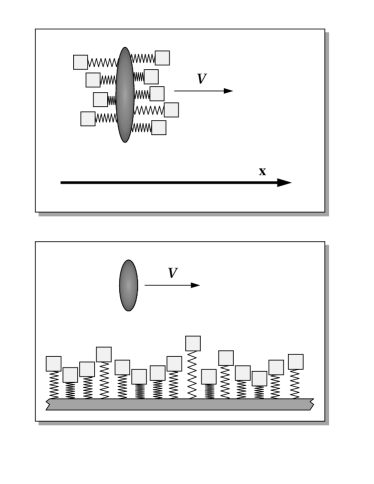
Figure 17: Schematic illustration of the ZCL model (upper panel) and the DLD model (lower panel). The Hamiltonian of these ”spring systems” is literally the ZCL model and the DLD model respectively. In the latter case the height of the masses should be interpreted as the ”height” of the potential which is experienced by the particle.

There is still some freedom left in the definition of the interaction with the harmonic bath. This leads to the introduction of the Diffusion-Localization-Dissipation (DLD) model dld ; gbm ; qbm . This model gives in the classical limit Brownian motion which is described by the standard Langevin equation (white noise + ohmic dissipation). The familiar Zwanzig-Caldeira-Leggett (ZCL) model zcl can be regarded as a special limit of the DLD model. The physics of the ZCL and of the DLD model is illustrated in Fig.16b and Fig.16c respectively, and the model Hamiltonians can be visualized by the drawings of Fig.17. The ZCL model describes a motion under the influence of a fluctuating homogeneous field of force which is induced by the environmental degrees of freedom. In case of the DLD model the induced fluctuating field is further characterized by a finite correlation distance.

For completeness we note that random-matrix modeling of the environment, in the regime where it has been solved blgc , leads to the same results as those obtained for the DLD model.

XVI System interacting with environment

The general problem of system that interacts with its environment is of great importance in many fields of physics. The basic ingredients of this interaction are illustrated in Fig.15. On the one hand we have the effect of dissipation, meaning that energy is lost by the ”system” (Brownian particle) and is absorbed by the ”environment” (gas particles). On the other hand the environment induces fluctuations that acts like ”noise” on the system. The ”noise” has two significant effects: One is to pump ”thermal” energy into the system, and the other is to spoil quantum coherence. The latter effect is called decoherence.

In case of bounded system, in the absence of external time dependent fields, the interplay between ”noise” and ”dissipation” leads eventually to ”thermalization”. One may say that in the thermal state the effect of dissipation is balanced by the energy which is pumped by the noise. Thus, both classically and quantum mechanically we have to distinguish between a ”damping” scenario and an ”equilibrium” situation. The thermalization process is traditionally described as ”irreversible”. On the other hand we have the issue of ”recurrences”. We discuss the latter issue in Section 20.

A systematic approach for the study of the dynamics of a ”system”, taking into account the influence of its environment, has been formulated by Feynman and Vernon FV . The state of the system is represented by the probability matrix $\rho(x^{\prime},x^{\prime\prime})$. It is assumed that initially the ”system” is prepared is some arbitrary state. Its state at a later time is obtained by a propagator $K(x^{\prime},x^{\prime\prime}|x^{\prime}_{0},x^{\prime\prime}_{0})$ which acts on the initial preparation. The calculation of this propagator involves a double path integral over all the possible trajectories $x_{A}(t)$ and $x_{B}(t)$ that connect $(x^{\prime}_{0},x^{\prime\prime}_{0})$ with $(x^{\prime},x^{\prime\prime})$. This double path integral incorporates the effect of the environment via an ”influence functional” which is defined as follows:

$$F[x_{A},x_{B}]\ \ =\ \ \langle\ U[x_{B}]\Psi_{0}\ |\ U[x_{A}]\Psi_{0}\ \rangle$$ (34)

Here $\Psi_{0}$ is the initial state of the environment. If the environment is in ”mixed” state, typically a canonical (thermal) state, then the influence functional should be averaged accordingly.

The absolute value of the influence functional can be re-interpreted as arising from the interaction with a c-number noisy field (with no back reaction). The ”phase” of the influence functional can be regarded as representing the effect of ”friction” (back reaction). Thus there is one to one correspondence between the Feynman-Vernon formalism, and the corresponding classical Langevin approach. Note however that the distinction between ”noise” and ”friction” is a matter of ”taste”. Some people regard this distinction meaningless.

It should be realized that the calculation of the influence functional for a given environment takes us back to the more restricted problem of considering a ”driven system”. The influence functional $F[x_{A},x_{B}]$ is nothing but the survival amplitude for a driving scheme that involves ”time reversal” (Eq.(15)).

XVII Entanglement, decoherence and irreversibility

The definition of decoherence is not a trivial matter conceptually. There are several equivalent ways to think about decoherence. The most ”robust” approach is to define decoherence as the irreversible entanglement of the system with the environment: Let us describe the the state of the system using the probability matrix $\rho(x^{\prime},x^{\prime\prime})$. If the system is prepared in pure state then $\mbox{trace}(\rho^{2})=1$. Due to the interaction with the environment the system gets entangled with the environment, and as a result we will have $\mbox{trace}(\rho^{2})\leq 1$. If the ”environment” consists of only ”one spin”, then we expect $\mbox{trace}(\rho^{2})$ to have ”ups” and ”downs”, and from time to time to have $\mbox{trace}(\rho^{2})\sim 1$. In such case we cannot say that the entanglement process is ”irreversible”. But if the environment consists of many degrees of freedom, as in the case of interaction with ”bath”, then the loss of ”purity” becomes irreversible, and we regard it as a ”decoherence process”.

To be more specific let us consider the prototype example of interference in Aharonov-Bohm ring geometry. The particle can go from the input lead to the output lead by traveling via either arms of the ring. This leads to interference, which can be tested by measuring the dependence of the transmission on the magnetic flux via the ring. Consider now the situation where there is a spin degree of freedom in one arm imry . The particle can cause a spin flip if it travels via this arm. In such case interference is lost completely. However, this entanglement process is completely reversible. We can undo the entanglement simply by letting the particle interact with the spin twice the time. Therefore, according to our restrictive definition, this is not a real decoherence process.

Consider now the situation where a particle gets entangled with bath degrees of freedom. If the bath is infinite, then the entanglement process is irreversible, and therefore it constitutes, according to our definition, a decoherence process.

At first sight it seems that for having irreversibility one needs ”infinity”. This point of view is emphasized in Ref.buttiker : Irreversibility can be achieved by having the infinity of the bath (infinitely many oscillators), or of space (a lead that extends up to infinity). In this set of lectures we emphasize a third possibility: Having irreversibility due to the interaction with chaos. Thus we do not need ”infinity” in order to have ”irreversibility”.

XVIII Interpretation of decoherence as a dephasing process

”Dephasing” is used as a synonym for ”decoherence” whenever a semiclassical point of view is adopted. Determining the dephasing (decoherence) time $\tau_{\varphi}$ for a particle $(x,p)$ that interacts with an environmental degrees of freedom $(Q,P)$ is a central theme in quantum physics. In the absence of such interaction the $x$ motion is coherent, and interference should be taken into account. This means, from semiclassical point of view, that at least two trajectories $x(\tau)=x_{\mbox{\tiny A}}(\tau)$ and $x(\tau)=x_{\mbox{\tiny B}}(\tau)$ have a leading contribution to the probability to travel, say, from $x(0)$ to $x(t)$, as in the prototype example of the two slit experiment.

In the semiclassical framework the probability to travel from one point to some other point is given by an expression that has the schematic form

$$\sum_{A,B}F[x_{A},x_{B}]\exp\left(i\frac{S[x_{A}]-S[x_{B}]}{\hbar}\right)$$ (35)

where $S[x]$ is the classical action, and $F[x_{A},x_{B}]$ is the influence functional. Each pair of trajectories is a ”stationary point” of the Feynman-Vernon double path integral. The ”diagonal terms” are the so-called classical contribution, while the ”off-diagonal terms” are the interference contribution. It should be kept is mind that the validity of the semiclassical approach is a subtle issue dph .

The off-diagonal interference contribution is suppressed due to the interaction with the environment if $|F[x_{A},x_{B}]|\ll 1$. Therefore $|F[x_{A},x_{B}]|$ is called the ”dephasing factor”. From the definition of the influence functional it is clear that it reflects the probability to ”leave a trace” in the environment. Having $|F[x_{A},x_{B}]|=0$ means that a different ”trace” is left in the environment, depending on whether the particle goes via the trajectory $x_{A}(t)$ or via the trajectory $x_{B}(t)$. In such case one can regard the interaction with the environment as a ”measurement” process. In case of the DLD model (see Section 15) this ”trace” can be further interpreted as leaving an excitation along the way. For critical discussion of this point see Appendix C of qbm . In the more general case the notion of ”leaving a trace” does not have a simple meaning. All we can say is that decoherence means that the environment is left in different (orthogonal) states depending on the trajectory that is taken by the particle.

The law of ”action and reaction” holds also in the world of decoherence studies. Feynman and Vernon have realized that the dephasing factor can be re-interpreted as representing the effect of a c-number noise source (see section 16). From this point of view the decoherence is due to the ”scrambling” of the relative phase by this noise. Hence the reason for using the term ”dephasing” as a synonym for ”decoherence”. The analysis of dephasing using this latter point of view can be found in qbm . See also alicki . At high temperatures it is possible to use a Markovian master equation approach (dynamical semigroups) in order to obtain the (reduced) evolution of the Brownian particle. The Markovian master equation approach is described in other lectures of this school. The master equation in case of the DLD model can be found in Section 3 of qbm . Similar, but not identical master equations are obtained in case of interaction with many body bath vacchini .

XIX Determination of the dephasing time

In the above described semiclassical framework, the problem of dephasing reduces to the more restricted problem of studying the dynamics of a time dependent Hamiltonian ${\cal H}(Q,P;x(t))$. Moreover, we see that the Feynman-Vernon dephasing factor is just the absolute value of the fidelity amplitude $F(t)$ that corresponds to Eq.(15). Note however that here we use a more general notion of fidelity: The restricted definition of fidelity (Eq.(17)) is formally obtained if $x_{\mbox{\tiny A}}(\tau)$ and $x_{\mbox{\tiny B}}(\tau)$ are ”rectangular pulses”.

The dephasing time $\tau_{\varphi}$ is defined as the time that it takes for $|F(t)|$ to drop significantly from $|F(t)|\sim 1$ to some very small value $|F(t)|\ll 1$. Let us concentrate on the Brownian motion model of Fig.16a. If the motion of the Brownian particle is characterized by a velocity $V$, then we have to distinguish between the following possibilities: Having very small ”adiabatic” velocities; Having intermediate velocities that allow LRT treatment; And having non-perturbative velocities. In the latter case a semiclassical picture can be justified.

The detailed analysis of the problem can be found in wld . Here we just quote the final results. In the semiclassical regime

$$\tau_{\varphi}\ =\ \tau_{\mbox{\tiny col}}\ =\ \frac{L_{\mbox{\tiny col}}}{v_{\mbox{\tiny E}}}$$ (36)

where $L_{\mbox{\tiny col}}$ is the mean free path between collisions with the Brownian particle. This is the expected naive result. It means that one collision with the Brownian particle is enough in order to ”measure” its trajectory. The other extreme case in having extremely small adiabatic velocities. To the extend that we can trust adiabaticity there is no dephasing at all: The gas particle simply ”renormalize” the bare potential, which is in fact the Born-Oppenheimer picture. Of course, if we take into account corrections to the adiabatic picture, then we get a finite dephasing time. In the LRT regime of velocities we can estimate the dephasing time as

$$\tau_{\varphi}\ \ \approx\ \ \left(\frac{L_{\mbox{\tiny col}}\lambda_{\mbox{\tiny E}}^{2}}{v_{\mbox{\tiny E}}V^{2}}\right)^{\frac{1}{3}}$$ (37)

Both results have re-interpretation within the framework of an effective DLD/ZCL model. See wld for details.

XX Recurrences

Consider ice-cube inside a cup of hot water. After some time it melts and disappears. But if we wait long enough (without time reversal) we have some probability to see the ice-cube re-emerging due to recurrences. The issue of recurrences becomes relevant whenever we consider a closed (un-driven) system. In other words, whenever we do not try to control its evolution from the outside.

There are recurrences both in classical and quantal physics. In the latter case the tendency for recurrences is stronger due to the quasi-periodic nature of the dynamics. However, if the time scale for recurrences is long enough with respect to other relevant time scales, then we can practically ignore these recurrences. Actually it is useful to regard these recurrences as ”fluctuations”, and to take the standpoint that our interest is only in some ”average” or ”likely” scenario.

The thermalization process of the particle-environment system is traditionally described as ”irreversible”. Indeed, if the bath is infinite, then also the time for recurrences of the particle-bath system becomes infinite. On the other hand, if the bath is finite, then we have to consider the recurrences of the particle-bath system. These recurrences can lead back to the initial un-entangled state.

In practice ”recurrences” do not constitute a danger for ”irreversibility”. The time to get un-entangled by recurrences is extremely large (typically larger than the age of the universe). Assuming a chaotic environment, and ignoring issues of level statistics, the time scale for recurrences is at least the Heisenberg time (inverse of the mean level spacing) of the combined particle-environment system. It scales like $\hbar^{-(d+d_{0})}$ where $d_{0}$ and $d$ are the number of degrees of freedom of the particle and the environment respectively.

It goes without saying that the above issue of recurrences becomes irrelevant if the $x$ motion is treated classically. There is however a twist to this latter statement in the case where the time variation of $x$ is strictly periodic. This is due to dynamical localization effect qkr . Note however that dynamical localization is a very fragile effect: Even in case that it is found, it turns out that it manifests itself only after a time that scales like $\hbar^{-(1+2d)}$, which is much larger than the Heisenberg time of the environment rsp .

Acknowledgments:

Essential for the promotion of this line of study are the collaborations with Tsampikos Kottos (MPI Gottingen), and with Alex Barnett (Harvard), and lately with Diego Wisniacki (Comision Nacional de Energia Atomica, Argentina). I also thank Shmuel Fishman (Technion) for many useful discussions, and Rick Heller (Harvard), Joe Imry (Weizmann), Bilha Segev (Ben-Gurion) and Uzy Smilansky (Weizmann) for interesting interaction.

Figure 2: The 1D version of the piston model (upper panel). The gas particle is moving inside an ”infinite well”. Its motion is not chaotic. In order to have chaotic motion we should consider at least a 2D box, for example a stadium shaped billiard system (lower panel).

Figure 3: Other versions of the ”piston model”. Two examples of ”Sinai billiards” are illustrated. Note that in case of the right panel the displacement of the wall element manifestly does not involve a change of volume. This feature simplifies the analysis.

Figure 4: The same ”Sinai billiards” as in the previous figure. Here the driving is achieved by changing the perpendicular magnetic field. In case of the left panel, where the box has a simple ”quantum dot” geometry, the magnetic field is assumed to be homogeneous. In case of the right panel, where the box has a aharonov-Bohm ring topology, the magnetic flux is assumed to be concentrated in the hole.

Figure 9: Various driving schemes: Rectangular pulse of duration $T$ and amplitude $A$; Triangular pulse which is further characterized by finite driving ”velocity” $V=|\dot{x}|=2A/T$; Periodic driving with frequency $\Omega=2\pi/T$.

Figure 10: Energy spreading as a function of time for the 2DW model: (a) classical; (b) quantum mechanical; (c) An effective Wigner model. The energy in these simulations is $E\sim 3$, and $\delta x=0.2123$. The light dashed lines in (a) and (c), that have slopes $1$ and $1/2$ respectively, are drawn to guide the eye. In (c) different lines correspond to different values of $\hbar$ as in (b), and additional curves ($\hbar=0.009,0.005$) have been added. Taken from Ref.wpk .

Figure 11: The dependence of the friction coefficient on the driving frequency, using LRT. ”GN” stands for generic deformation of a stadium shaped billiard, while ”DI” stands for special deformation (dilation). [In the latter case the friction coefficient vanishes in the low frequency limit.] In both cases the agreement between the classical (solid line) and the quantum-mechanical (dashed line) calculation is remarkable. Taken from Ref.dil .

Figure 12: The dependence of the mesoscopic conductance on the driving frequency. The calculation is done for a Sinai billiard shaped quantum dot, using LRT. The result can be regarded as a mesoscopic version of Drude formula. The specific geometry of the system is reflected in the structure of the response curve. The inset is log-log plot. Taken from Ref.wlf .

Figure 13: The response of a quantum mechanical system is displayed as a function of $A$ and $\Omega$. The simulations are done for Wigner model with periodic driving. The units are chosen such that $\Delta=0.5$ and $\hbar=1$ and $\sigma=1$. Upper panel: Plots of $D_{\mbox{\tiny E}}/A^{2}$ versus $\Omega/\omega_{\mbox{\tiny cl}}$ for few values of $A$. For small $\omega$ the plots coincide as expected from LRT. As $A$ becomes larger the deviations from LRT scaling become more pronounced, and we get response also for $\Omega>\omega_{\mbox{\tiny cl}}$. Lower panel: Plots of $D_{\mbox{\tiny E}}/D_{0}$ versus $A/\sqrt{b}$ for few values of $\Omega/\omega_{\mbox{\tiny cl}}$. LRT implies $D_{\mbox{\tiny E}}/D_{0}=1$ for $\Omega/\omega_{\mbox{\tiny cl}}<1$ and $D_{\mbox{\tiny E}}/D_{0}=0$ for $\Omega/\omega_{\mbox{\tiny cl}}>1$. The purpose of the horizontal scaling is to demonstrate that $A_{\mbox{\tiny prt}}$ rather than $A_{c}$ is responsible for the deviation from this LRT expectation. Taken from Ref.rsp .

Figure 14: Upper diagram: The various $V$ regimes in the theory of driven systems for linear driving $x(t)=Vt$. Lower diagram: The various $(\Omega,A)$ regimes for periodic driving $x(t)=A\sin(\Omega t)$. We use the notations $\omega_{cl}=2\pi/\tau_{cl}$ and $A_{c}=\delta x_{c}$ and $A_{\mbox{\tiny prt}}=\delta x_{\mbox{\tiny prt}}$.

Figure 15: Block diagram illustrating the interaction between system ($x$) and environmental ($Q$) degrees of freedom (DoF). See discussion in the text.

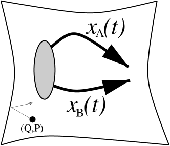
Figure 18: Schematic illustration of an interference experiment using a semiclassical point of view. The Brownian particle can take either the $x=x_{A}(t)$ trajectory, or the $x=x_{B}(t)$ trajectory as in a two slit experiment.

References

- (1) M.C. Gutzwiller, Chaos in Classical and Quantum Mechanics (Springer Verlag New York 1990).
- (2) H.J. Stockmann, ”Quantum Chaos : An Introduction” (Cambridge Univ Pr 1999).
- (3) F. Haake, ”Quantum Signatures of Chaos” (Springer 2000).
- (4) M. Wilkinson, J. Phys. A 21, 4021 (1988); J. Phys. A 20, 2415 (1987).
-
(5)
M. Wilkinson and E.J. Austin,
J. Phys. A 28, 2277 (1995).
E.J. Austin and M. Wilkinson, Nonlinearity 5, 1137 (1992). - (6) For review and references see qkr1 and qkr2 .
- (7) S. Fishman in ”Quantum Chaos”, Proceedings of the International School of Physics ”Enrico Fermi”, Course CXIX, Ed. G. Casati, I. Guarneri and U. Smilansky (North Holland 1991).
- (8) M. Raizen in ”New directions in quantum chaos”, Proceedings of the International School of Physics ”Enrico Fermi”, Course CXLIII, Edited by G. Casati, I. Guarneri and U. Smilansky (IOS Press, Amsterdam 2000).
- (9) D. Cohen in ”New directions in quantum chaos”, Proceedings of the International School of Physics ”Enrico Fermi”, Course CXLIII, Edited by G. Casati, I. Guarneri and U. Smilansky, (IOS Press, Amsterdam 2000).
- (10) D. Cohen, Phys. Rev. Lett. 82, 4951 (1999).
- (11) D. Cohen and T. Kottos, Phys. Rev. Lett. 85, 4839 (2000).
- (12) D. Cohen, Annals of Physics 283, 175 (2000).
- (13) D. Cohen, F.M. Izrailev and T. Kottos, Phys. Rev. Lett. 84, 2052 (2000).
- (14) T. Kottos and D. Cohen, Phys. Rev. E 64, R-065202 (2001).
- (15) S.W. Doescher and M.H. Rice, Am. J. Phys. 37, 1246 (1969).
- (16) A.J. Makowski and S.T. Dembinski, Physics Letters A 154, 217 (1991).
- (17) J.V. Jose and R. Cordery, Phys. Rev. Lett. 56, 290 (1986).
-
(18)
J. Blocki, Y. Boneh, J.R. Nix,
J. Randrup, M. Robel, A.J. Sierk and W.J. Swiatecki,
Ann. Phys. 113, 330 (1978). -
(19)
S.E. Koonin, R.L. Hatch and J. Randrup,
Nuc. Phys. A 283, 87 (1977).
S.E. Koonin and J. Randrup, Nuc. Phys. A 289, 475 (1977). - (20) D. Cohen and T. Kottos, Phys. Rev. E 63, 36203 (2001).
- (21) E. Wigner, Ann. Math 62 548 (1955); 65 203 (1957).
- (22) G. Casati, B.V. Chirikov, I. Guarneri, F.M. Izrailev, Phys. Rev. E 48, R1613 (1993); Phys. Lett. A 223, 430 (1996).
- (23) Y. Imry, Introduction to Mesoscopic Physics (Oxford Univ. Press 1997).
- (24) Y. Alhassid, Rev. Mod. Phys. 72, 895 (2000).
- (25) L.P. Kouwenhoven, C.M. Marcus, P.L. Mceuen, S. Tarucha, R. M. Westervelt and N.S. Wingreen, Proc. of Advanced Study Inst. on Mesoscopic Electron Transport, edited by L.L. Sohn, L.P. Kouwenhoven and G. Schon (Kluwer 1997).
- (26) M.V. Berry in Chaos and Quantum Systems, ed. M.-J. Giannoni, A. Voros, J. Zinn-Justin (Elsevier, Amsterdam, 1991).
- (27) M. Feingold and A. Peres, Phys. Rev. A 34 591, (1986). M. Feingold, D. Leitner, M. Wilkinson, Phys. Rev. Lett. 66, 986 (1991); M. Wilkinson, M. Feingold, D. Leitner, J. Phys. A 24, 175 (1991); M. Feingold, A. Gioletta, F. M. Izrailev, L. Molinari, Phys. Rev. Lett. 70, 2936 (1993).
- (28) H. Attias and Y. Alhassid, Phys. Rev. E 52, 4776 (1995).
- (29) T. Guhr, A. Muller-Groeling and H.A. Weidenmuller, Phys. Rep. 299, 190 (1998).
- (30) D. Cohen and E.J. Heller, Phys. Rev. Lett. 84, 2841 (2000).
- (31) D. Cohen, A. Barnett and E.J. Heller, Phys. Rev. E 63, 46207 (2001).
- (32) F. Borgonovi, I. Guarneri and F.M. Izrailev, Phys. Rev. E 57, 5291 (1998). L. Benet, F.M. Izrailev, T.H. Seligman and A. Suarez-Moreno, chao-dyn/9912035, Phys Lett A 277 (2000) 87-93.
- (33) E.J. Heller in Chaos and Quantum Systems, ed. M.-J. Giannoni, A. Voros, J. Zinn-Justin (Elsevier, Amsterdam, 1991).
- (34) A. Peres, Phys. Rev. A 30, 1610 (1984). See also A. Peres, Quantum Theory: Concepts and Methods (Dordrecht, 1995).
- (35) R.A. Jalabert and H.M. Pastawski, Phys. Rev. Lett. 86, 2490 (2001). F. M. Cucchietti, H. M. Pastawski, R. Jalabert Physica A, 283, 285 (2000). F.M. Cucchietti, H.M. Pastawski and D.A. Wisniacki, Phys. Rev. E 65, 045206(R) (2002). F. Cucchietti et al, nlin.CD/0112015.
- (36) Ph. Jacquod, P.G. Silvestrov and C.W.J. Beenakker, Phys. Rev. E 64, 055203 (2001).
- (37) N.R. Cerruti and S. Tomsovic, Phys. Rev. Lett. 88, 054103 (2002).
- (38) D.A. Wisniacki and D.Cohen, quant-ph/0111125, Phys. Rev. E 66, 046209 (2002)
- (39) T. Prosen, quant-ph/0106149. T. Prosen and M. Znidaric, J.Phys.A 34, L681 (2001).
- (40) T. Kottos and D. Cohen, cond-mat/0201148, Europhysics Letters 61, 431-437 (2003)
- (41) See frc and vrn . The classical theory that is presented in those references integrates ideas that were promoted in previous studies, mainly ott and wilk and jar93 .
- (42) E. Ott, Phys. Rev. Lett. 42, 1628 (1979). R. Brown, E. Ott and C. Grebogi, Phys. Rev. Lett, bf 59, 1173 (1987); J. Stat. Phys. 49, 511 (1987).
- (43) C. Jarzynski, Phys. Rev. E 48, 4340 (1993).
- (44) A clear formulation of the diffusion dissipation relation can be found in vrn ; frc , and also in Appendix A of wlf . It constitutes a refinement/generalization of the dissipation picture which is presented in wilk . The standard textbook formulation of LRT and the fluctuation-dissipation relation can be found in Appendix A of imry .
- (45) A. Barnett, D. Cohen and E.J. Heller, J. Phys. A 34, 413 (2001).
- (46) D. Cohen, unpublished.
- (47) A. Barnett, D. Cohen and E.J. Heller, Phys. Rev. Lett. 85, 1412 (2000).
-
(48)
J.M. Robbins and M.V. Berry,
J. Phys. A 25, L961 (1992).
M.V. Berry and J.M. Robbins, Proc. R. Soc. Lond. A 442, 659 (1993).
M.V. Berry and E.C. Sinclair, J. Phys. A 30, 2853 (1997). - (49) O.M. Auslaender and S. Fishman, Phys. Rev. Lett. 84, 1886 (2000); J. Phys. A 33, 1957 (2000).
- (50) D.A. Wisniacki and E. Vergini, Phys. Rev. E 59, 6579 (1999).
- (51) C. Jarzynski, Phys. Rev. Lett. 74, 2937 (1995).
- (52) D. Cohen, Phys. Rev. E 55, 1422 (1997).
- (53) D. Cohen, Phys. Rev. Lett. 78, 2878 (1997).
- (54) D. Cohen, J. Phys. A 31, 8199 (1998).
-
(55)
A.O. Caldeira and A.J. Leggett,
Physica 121 A, 587 (1983).
A.O. Caldeira and A.J. Leggett, Ann. Phys. (N.Y.)
140, 374 (1983);
Physica 121 A, 587 (1983). - (56) L. Bonig, K. Schonhammer and W. Zwerger, Phys. Rev. B 46, 855 (1992).
- (57) B. Vacchini, Phys. Rev. E 63, 066115 (2001); J. Math. Phys. 42, 4291 (2001).
- (58) A. Bulgac, G.D. Dang and D. Kusnezov, Phys. Rev. E 58, 196 (1998).
- (59) R.P. Feynman and F.L. Vernon Jr., Ann. Phys. (N.Y.) 24, 118 (1963).
- (60) M. Buttiker, cond-mat/0106149, in p.21-47 of ”Complexity from Microscopic to Macroscopic Scales: Coherence and Large Deviations”, edited by Arne T. Skjeltorp and Tamas Vicsek (Kluwer, Dordrecht 2002).
- (61) D. Cohen and Y. Imry, Phys. Rev. B 59, 11143 (1999).
- (62) D. Cohen, Phys. Rev. E 65, 026218 (2002).
- (63) R. Alicki, Phys. Rev. A 65, 034104 (2002).
-
(64)
For follow up studies see
http://www.bgu.ac.il/dcohen/