Coherent backscattering of light by atoms in the saturated regime

Abstract

We present the first calculation of coherent backscattering with inelastic scattering by saturated atoms. We consider the scattering of a quasi-monochromatic laser pulse by two distant atoms in free space. By restricting ourselves to scattering of two photons, we employ a perturbative approach, valid up to second order in the incident laser intensity. The backscattering enhancement factor is found to be smaller than two (after excluding single scattering), indicating a loss of coherence between the doubly scattered light emitted by both atoms. Since the undetected photon carries information about the path of the detected photon, the coherence loss can be explained by a which-path argument, in analogy with a double-slit experiment.

PACS numbers: 42.25.Fx, 32.80-t, 42.50-p

I Introduction

Weak localization of light in random media was demonstrated for the first time in the eighties [1, 2, 3]. Here, constructive interference between two waves which interact with the same particles, but in reversed order, enhances, in average, scattering in the direction opposite to the incident light. For systems obeying the reciprocity symmetry [4], the backscattering enhancement factor, i.e. the light intensity detected in exact backscattering direction divided by the background intensity, is exactly two, provided single scattering can be removed. For spherically symmetric scatterers, the latter is achieved in the helicity preserving polarization channel.

Similar interference effects between multiply scattered waves also affect the properties of transport through disordered media. If the mean free path can be sufficiently reduced, the transport is even expected to come to a complete standstill [5]. In experiments on strong localization of light [6], however, the role of absorption is discussed controversially [7, 8].

One may wonder whether a medium consisting of individual atoms would constitute a good candidate for strong localization. In contrast to the classical scenario (Maxwell’s equations in a medium with random dielectric constant), the quantum-mechanical atom-photon interaction exhibits some characteristic features, which may affect the coherence between multiply scattered waves. Firstly, the resonance may be extremely sharp, corresponding to a very narrow linewidth $\Gamma$ of the excited state. On the one hand, this leads to a large atom-photon scattering cross section and slow diffusion of light [9] - properties in favor of localization. On the other hand, it implies that the atoms have to be cooled to very low temperatures. Only if the Doppler shift induced by a moving atom is much smaller than $\Gamma$, the interference between two counterpropagating waves is preserved [10]. Typically, this regime is reached at about a few $\rm mK$, which is, however, still high enough to neglect the thermal de-Broglie wavelength of the atoms, i.e. to treat their external motion classically. Furthermore, atoms usually have an internal quantum structure, which may have a strong impact on coherent backscattering [11, 12, 13, 14]. If necessary, this can be circumvented by using atoms with a nondegenerate ground state ($J=0$) [15].

Another property of the atom-light interaction, whose impact on coherent backscattering has so far remained almost unexplored, is the strongly nonlinear response of an atom to incoming radiation. A single photon being sufficient to bring the atom to the excited state, where it rests for a quite long time $\Gamma^{-1}$ without being able to scatter other photons, a saturation of the atomic medium can be induced already with rather moderate laser intensities. Not only the atom-photon cross section, but also the spectrum of the light is affected by saturation. With increasing saturation, it becomes more and more probable that an atom scatters inelastically, i.e. that it emits photons at a frequency different from the one of the incident laser. As we will show in this paper, this implies a loss of coherence between two reversed scattering paths. Similarly, a recent experiment showed coherent backscattering by a cloud of cold Strontium atoms to be reduced when increasing the saturation induced by the probe laser [16].

In order to expose the physical mechanism responsible for the loss of coherence as clearly as possible, we will consider in this paper two two-level atoms in free space - the simplest system exhibiting coherent backscattering. Effects which arise in the presence of a larger number of atoms, such as the nonlinear index of refraction of an atomic medium, will be relegated to future publications. Furthermore, we assume that the distance between the two atoms is much larger than the optical wavelength, such that we can neglect recurrent scattering (corresponding to a dilute medium in the case of many atoms). To calculate the photodetection signal of the light emitted by the two atoms, we use scattering theory. Generally, the higher the intensity of the incoming light, the more photons are scattered inelastically. In the present paper, we restrict ourselves to two-photon scattering. Thereby, we employ a perturbative approach, valid up to second order in the incident intensity.

The paper is organized as follows. In Sec. II, we summarize known results about the scattering of two photons by a single atom. After introducing the scattering operator in Sec. II B, we obtain the corresponding photodetection signal in Sec. II C, thereby recovering the resonance fluorescence spectrum in second order of the intensity. In Sec. III, we add a second atom to our model. We proceed in a similar way as in Sec. II, using the results of the single-atom case as a building block of the two-atom solution. After deriving the scattering operator in Sec. III A, we calculate the photodetection signal in Sec. III B. In contrast to the single-atom case, the latter contains interference between the light emitted by the two atoms, enhancing the detection signal in the backscattering direction. In this way, we obtain the main result of the present paper, the backscattering enhancement factor, which is found to be smaller than two, due to inelastic scattering. This fact is interpreted in Sec. III C as a loss of coherence between the light scattered by both atoms in opposite order. Regarding the undetected photon as a path detector for the detected photon, we can explain the loss of coherence by an analogy to the double-slit experiment, where the interference pattern is washed out if we try to observe which slit the particle has passed through. Finally, Sec. III D concludes the paper.

II Single atom

Let us start with discussing the scattering of two photons by a single atom. This is useful since we will assume later that the second atom is far away from the first one. The two-atom scattering process can then be viewed at as a succession of two single-atom scattering processes.

A Approximations and Hamiltonian

We assume a two-level atom located at a fixed position ${\bf r}$. As already mentioned above, neglecting the external atomic motion is justified at very low temperatures, where the Doppler shift induced by the atomic motion is small enough. Also the recoil effect, i.e. the change of the atomic velocity when scattering a photon, can be neglected - provided that the number of scattering events is not too large. On the other hand, the temperature should still be high enough such that the external atomic motion need not to be treated quantum mechanically. Furthermore, let us stress that we consider an undegenerate atomic ground state ($J=0$). This is important since coherent backscattering may be severely affected by degeneracy [11, 12, 13, 14]. The excited state is then threefold degenerate ($J=1$). Which one of the three excited states is populated depends on the polarization of the absorbed photon.

With the approximations mentioned above, our Hamiltonian reads as follows:

$$H=H_{0}+V,$$ (1)

where

$$H_{0} = \tilde{\omega}_{\rm at}\sigma^{\dagger}\sigma+\sum_{{\bf k},s}\omega_{\bf k}a_{{\bf k}s}^{\dagger}a_{{\bf k}s},$$ (2)

$$V = \sum_{{\bf k},s}\left(ige^{i{\bf k}{\bf r}}(\sigma^{\dagger}\cdot\epsilon_{{\bf k}s})a_{{\bf k}s}-ige^{-i{\bf k}{\bf r}}(\sigma\cdot\epsilon^{*}_{{\bf k}s})a^{\dagger}_{{\bf k}s}\right),$$ (3)

denote the free evolution, and the interaction, respectively (in units where $\hbar=1$). Here, the operators $\sigma^{\dagger}$ and $\sigma$ describe transitions between the atomic ground and excited states, with energy difference $\tilde{\omega}_{\rm at}$ (in the case of an isolated atom), whereas $a_{{\bf k}s}^{\dagger}$ and $a_{{\bf k}s}$ create and annihilate a photon in mode $\bf k$ (a plane wave with wavevector $\bf k$) and polarization $\epsilon_{{\bf k}s}$ (perpendicular to $\bf k$). The coupling constant

$$g=d\left(\frac{\omega_{\bf k}}{2\epsilon_{0}L^{3}}\right)^{1/2}\simeq d\left(\frac{\omega_{\rm at}}{2\epsilon_{0}L^{3}}\right)^{1/2},$$ (4)

with $L^{3}$ the quantization volume (which will finally drop out of the equations, when taking the limit $L\to\infty$) and $d$ the magnitude of the atomic dipole, determines the strength of the atom-field coupling.

In Eq. (3), we have employed the so-called ‘rotating wave approximation’: a transition from one of the excited states to the ground state is only possible by emitting a photon, and vice versa by absorption. This is justified since we will restrict ourselves to near-resonant processes, where only photons with frequencies close to the atomic resonance are important (i.e. $|\omega_{\bf k}-\omega_{\rm at}|\ll\omega_{\rm at}$). For the same reason, we may assume a constant value of $g$ in Eq. (4), i.e. neglect its dependence on $\omega_{\bf k}$.

Due to the coupling to the electromagnetic vacuum, the state $|e\rangle$ is unstable: after an average lifetime given by

$$\Gamma=\frac{d^{2}\omega_{\rm at}^{3}}{3\pi\epsilon_{0}}=\frac{2g^{2}\omega_{\rm at}^{2}L^{3}}{3\pi},$$ (5)

an excited atom decays into the ground state, through spontaneous emission of a photon. This gives rise to an effective, complex atomic resonance frequency

$$\omega_{0}=\omega_{\rm at}-i\frac{\Gamma}{2},$$ (6)

where also the real part $\omega_{\rm at}$ is shifted, as compared to the isolated atom, Eq. (2).

B Scattering matrix

In the following, we make use of scattering theory in order to calculate the properties of the light emitted by the atoms. Here, the object of interest is the scattering operator $S$, which connects the initial and final photon states $|i\rangle$ and $|f\rangle$:

$$|f\rangle=S|i\rangle.$$ (7)

The initial and final state of the atom is always the ground state $|g\rangle$, which we do not explicitly write in the following. Furthermore, we will restrict ourselves to the scattering of two photons, thereby employing a perturbative approach, valid up to second order in the incident intensity.

Since, as we will see below, the two photons may be scattered independently from each other, we consider first the scattering of a single photon. In order to distinguish between the scattered and non-scattered part of the photon wavepacket, the transition operator $T_{1}$ is introduced as follows:

$$S_{1}={\mathbbm{1}}-2\pi i\delta(\omega_{f}-\omega_{i})T_{1},$$ (8)

where the $\delta$-function implies conservation of the photon’s frequency (which follows from energy conservation, since the state of the atom is the same before and after scattering). For one-photon states, its matrix elements read [17]:

$$\langle{\bf k}_{f}\epsilon_{f}|T_{1}|{\bf k}_{i}\epsilon_{i}\rangle=\frac{g^{2}}{\omega_{i}-\omega_{0}}(\epsilon_{i}\cdot\epsilon_{f}^{*})e^{i({\bf k}_{i}-{\bf k}_{f})\cdot{\bf r}}.$$ (9)

The situation changes when considering a second photon. It is convenient to write the matrix elements in the following form:

$$\langle{\bf k_{3}}\epsilon_{3},{\bf k_{4}}\epsilon_{4}|S_{2}|{\bf k_{1}}\epsilon_{1},{\bf k_{2}}\epsilon_{2}\rangle =$$ (13)

$$\!\!\!\!\!\!\!\!\!\!\!\!\!\!\!\!\!\!\!\!\!\!\!\!\!\!\!\!\!\!\!\!\!\!\!\!\!\!\!\!\!\!\!\!\!\!\!\!\!\!\!\!\!\!\!\!\!\!\!\!\!\!\!\!\langle{\bf k_{3}}\epsilon_{3}|S_{1}|{\bf k_{1}}\epsilon_{1}\rangle\langle{\bf k_{4}}\epsilon_{4}|S_{1}|{\bf k_{2}}\epsilon_{2}\rangle$$

$$\!\!\!\!\!\!\!\!\!\!\!\!\!\!\!\!\!\!\!\!\!\!\!\!\!\!\!\!\!\!\!\!+\langle{\bf k_{3}}\epsilon_{3}|S_{1}|{\bf k_{2}}\epsilon_{2}\rangle\langle{\bf k_{4}}\epsilon_{4}|S_{1}|{\bf k_{1}}\epsilon_{1}\rangle$$

$$\!\!\!\!\!\!\!\!\!\!\!\!\!\!\!\!\!\!\!\!\!\!\!\!\!\!\!\!\!\!\!\!\!\!\!\!\!\!\!\!\!\!\!\!\!\!\!\!\!\!\!\!\!\!\!\!\!\!\!\!\!\!\!\!+\langle{\bf k_{3}}\epsilon_{3},{\bf k_{4}}\epsilon_{4}|T_{2}|{\bf k_{1}}\epsilon_{1},{\bf k_{2}}\epsilon_{2}\rangle.$$

Here, the first two terms scatter the two photons independently from each other. (There are two terms since the photons are indistinguishable: the final photon $|{\bf k_{3}}\epsilon_{3}\rangle$, for example, may correspond either to the initial photon $|{\bf k_{1}}\epsilon_{1}\rangle$ or $|{\bf k_{2}}\epsilon_{2}\rangle$.) Since, however, the atom cannot interact with the second photon while it is excited by the first one, the photons are in fact not completely independent. This gives rise to the second term [18]:

$$\langle{\bf k_{3}}\epsilon_{3},{\bf k_{4}}\epsilon_{4}|T_{2}|{\bf k_{1}}\epsilon_{1},{\bf k_{2}}\epsilon_{2}\rangle =$$ (16)

$$\!\!\!\!\!\!\!\!\!\!\!\!\!\!\!\!\!\!\!\!\!\!\!\!\!\!\!\!\!\!\!\!\!\!\!\!\!\!\!\!\!\!\!\!\!\!\!\!\!\!\!\!\!\!\!\!\!\!\!\!\!\!\!\!\!\!\!\!\!\!\!\!\!\!2\pi i\frac{g^{4}\delta(\omega_{1}+\omega_{2}-\omega_{3}-\omega_{4})}{(\omega_{1}-\omega_{0})(\omega_{2}-\omega_{0})}\left(\frac{1}{\omega_{3}-\omega_{0}}+\frac{1}{\omega_{4}-\omega_{0}}\right)$$

$$\!\!\!\!\!\!\!\!\!\!\!\!\!\!\!\!\!\!\!\!\!\!\!\!\!\!\!\!\!\!\!\!\!\!\!\!\!\!\!\!\!\!\!\!\!\!\!\!\!\!\!\!\!\!\!\!\!\!\!\!\!\!\!\!\!\!\!\!\!\!\!\!\![(\epsilon_{1}\cdot\epsilon_{3}^{*})(\epsilon_{2}\cdot\epsilon_{4}^{*})+(\epsilon_{2}\cdot\epsilon_{3}^{*})(\epsilon_{1}\cdot\epsilon_{4}^{*})]e^{i({\bf k}_{1}+{\bf k}_{2}-{\bf k}_{3}-{\bf k}_{4})\cdot{\bf r}}.$$

Although their sum is conserved, the individual frequencies of both photons may be changed by $T_{2}$, for what reason we call it ‘inelastic’ scattering.

C Photodetection signal

Given the final photon state $|f\rangle$, the intensity of the photodetection signal, as measured by a broadband detector (polarization $\epsilon_{D}$) located at ${\bf R}$ at time $t$ reads [17]:

$$I=\langle f|E^{(-)}({\bf R},t)E^{(+)}({\bf R},t)|f\rangle.$$ (17)

Here, the detection of the photon is described by the electric field operator

$$E^{(+)}({\bf R},t)=\frac{g}{d}\sum_{{\bf k},s}(\epsilon_{{\bf k}s}\cdot\epsilon_{D}^{*})e^{i({\bf k}\cdot{\bf R}-\omega t)}a_{{\bf k}s},$$ (18)

which annihilates a photon at position ${\bf R}$.

As initial state, we consider a state of $N$ photons

$$|i_{N}\rangle=\sqrt{N!}\sum_{({\bf k}_{1}\dots{\bf k}_{N})}h({\bf k}_{1})\dots h({\bf k}_{N})|{\bf k}_{1}\epsilon_{L},\dots,{\bf k}_{N}\epsilon_{L}\rangle,$$ (19)

where all photons are described by the same single-photon wavepacket

$$|i_{1}\rangle=\sum_{\bf k}h({\bf k})|{\bf k}\epsilon_{L}\rangle.$$ (20)

The factor $\sqrt{N!}$ in Eq. (19) arises from the symmetry under exchange of photons as bosonic particles, and is required to obtain the correct normalization, $\langle i_{N}|i_{N}\rangle=\langle i_{1}|i_{1}\rangle=1$. We assume that the wavepacket describes an almost plane wave, i.e., $h(\bf k)$ is sharply peaked around its center ${\bf k}_{L}$ (‘sharply’ means: much narrower than $\Gamma$). For this reason, we may also neglect in Eq. (19) the dependence of the initial polarization vector $\epsilon_{L}$ on $\bf k$.

The initial state $|i_{N}\rangle$ corresponds to the following incident intensity seen by the atom at position ${\bf r}$ and time $t=0$, obtained by inserting $|i_{N}\rangle$ instead of $|f\rangle$ in Eq. (17), and summing over the detector polarization $\epsilon_{D}$:

$$I_{\rm in}=N\frac{g^{2}}{d^{2}}\Biggl{|}\sum_{\bf k}e^{i{\bf k}\cdot{\bf r}}h({\bf k})\Biggr{|}^{2}.$$ (21)

In the following, we will use a dimensionless quantity, the so-called ‘saturation parameter’

$$s=\frac{2d^{2}I_{\rm in}}{|\omega_{L}-\omega_{0}|^{2}}=\frac{2Ng^{2}}{|\omega_{L}-\omega_{0}|^{2}}\Biggl{|}\sum_{\bf k}e^{i{\bf k}\cdot{\bf r}}h({\bf k})\Biggr{|}^{2}.$$ (22)

It accounts for the fact that photons interact less strongly with the atom if they are far detuned from the atomic resonance (i.e. if $|\omega_{L}-\omega_{0}|$ is large). From the solution of the optical Bloch equations [17], it is known that $s$ determines the ratio between inelastic and elastic scattering, see Eq. (47) below.

We are interested in the photodetection signal measured at position ${\bf R}$ at time $t=|{\bf R}-{\bf r}|$ (the time needed for the scattered light to reach the detector, in units where $c=1$). We assume that the detector is placed far away from the atom, such that $t=|{\bf R}-{\bf r}|$ is long enough for the scattering approach to be valid. Furthermore, the detector should not be placed in the direction of the initial wavevector ${\bf k}_{L}$, such that only scattered photons are detected (i.e. $E^{(+)}({\bf R},t)|i_{1}\rangle=0$).

In order to proceed, we have to generalize the scattering operator for two photons, Eq. (13), to the case of $N$ photons. For this purpose, we assume that the saturation parameter $s$ is so small that at most one photon pair is scattered inelastically. This yields the photodetection signal up to second order in $s$, see below. Summing over the different pairs $(i,j)$, and taking into account all possible permutations of the $N$ photons, we obtain:

$$\langle{\bf k}_{1}^{\prime}\dots{\bf k}_{N}^{\prime}|S_{N}|{\bf k}_{1}\dots{\bf k}_{N}\rangle = \sum_{P_{N}}\prod_{l=1}^{N}\langle{\bf k}_{l}^{\prime}|S_{1}|{\bf k}_{P_{N}(i)}\rangle~{}+$$ (24)

$$\!\!\!\!\!\!\!\!\!\!\!\!\!\!\!\!\!\!\!\!\!\!\!\!\!\!\!\!\!\!\!\!\!\!\!\!\!\!\!\!\!\!\!\!\!\!\!\!\!\!\!\!\!\!\!\!\!\!\!\!\!\!\!\!\!\!\!+\sum_{\stackrel{{\scriptstyle\scriptstyle i,j=1}}{{i<j}}}^{N}\sum_{P_{N}/P_{2}}\langle{\bf k}_{i}^{\prime}{\bf k}_{j}^{\prime}|T_{2}|{\bf k}_{P_{N}(i)}{\bf k}_{P_{N}(j)}\rangle\prod_{\stackrel{{\scriptstyle\scriptstyle l=1}}{{l\neq i,j}}}^{N}\langle{\bf k}_{l}^{\prime}|S_{1}|{\bf k}_{P_{N}(l)}\rangle.$$

(In the following, we do not write explicitly the polarization vectors.) Eq. (24) contains a sum over all permutations $P_{N}$ of the $N$ indices $\{1\dots N\}$, modulo a permutation of the two indices $P_{N}(i)$ and $P_{N}(j)$ in the second term, where the latter permutation is included in the two-photon operator $T_{2}$, see Eq. (16). In the case $N=2$, the above expression agrees with the one of the previous section, Eq. (13). According to Eq. (24), the final photon state $|f_{N}\rangle=S_{N}|i_{N}\rangle$ can be expressed as follows:

$$\langle{\bf k}_{1}\dots{\bf k}_{N}|f_{N}\rangle = \sqrt{N!}\prod_{l=1}^{N}\langle{\bf k}_{l}|f_{1}\rangle+$$ (25)

$$+ \sqrt{\frac{N!}{2}}\sum_{\stackrel{{\scriptstyle\scriptstyle i,j=1}}{{i<j}}}^{N}\langle{\bf k}_{i}{\bf k}_{j}|g_{2}\rangle\prod_{\stackrel{{\scriptstyle\scriptstyle l=1}}{{l\neq i,j}}}^{N}\langle{\bf k}_{l}|f_{1}\rangle,$$ (26)

in terms of the one- and two-photon states

$$|f_{1}\rangle = S_{1}|i_{1}\rangle,$$ (27)

$$|g_{2}\rangle = T_{2}|i_{2}\rangle.$$ (28)

Following Eq. (17), we now apply the electric field operator on the final photon state. It may annihilate either an elastically or an inelastically scattered photon. Correspondingly, we obtain the following three contributions:

$$|\psi\rangle=E^{(+)}({\bf R},t)|f\rangle=\sum_{i=1}^{3}|\psi_{i}\rangle,$$ (29)

with

$$\langle{\bf k}_{1}\dots{\bf k}_{N-1}|\psi_{1}\rangle = \sqrt{N!}E\prod_{l=1}^{N-1}\langle{\bf k}_{l}|f_{1}\rangle,$$ (30)

$$\langle{\bf k}_{1}\dots{\bf k}_{N-1}|\psi_{2}\rangle = \sqrt{\frac{N!}{2}}\sum_{i=1}^{N-1}\langle{\bf k}_{i}|g_{1}\rangle\prod_{\stackrel{{\scriptstyle\scriptstyle l=1}}{{l\neq i}}}^{N-1}\langle{\bf k}_{l}|f_{1}\rangle,$$ (31)

$$\langle{\bf k}_{1}\dots{\bf k}_{N-1}|\psi_{3}\rangle = \sqrt{\frac{N!}{2}}E\sum_{\stackrel{{\scriptstyle\scriptstyle i,j=1}}{{i<j}}}^{N-1}\langle{\bf k}_{i}{\bf k}_{j}|g_{2}\rangle\prod_{\stackrel{{\scriptstyle\scriptstyle l=1}}{{l\neq i,j}}}^{N-1}\langle{\bf k}_{l}|f_{1}\rangle,$$ (32)

and

$$E = \langle 0|E^{(+)}({\bf R},t)|f_{1}\rangle,$$ (33)

$$|g_{1}\rangle = E^{(+)}({\bf R},t)|g_{2}\rangle.$$ (34)

According to Eq. (17), the norm $I=\langle\psi|\psi\rangle$ gives the total intensity. Let us first concentrate on the contributions from $|\psi_{1}\rangle$ and $|\psi_{2}\rangle$. (As we will argue later, $|\psi_{3}\rangle$ can be neglected). We obtain a sum of three terms, from elastic and inelastic scattering, and their interference. Using $\langle f_{1}|f_{1}\rangle=1$ (since $S_{1}$ is unitary), we obtain:

$$I_{\rm el}^{(1)} = \langle\psi_{1}|\psi_{1}\rangle=N|E|^{2},$$ (35)

$$I_{\rm el}^{(2)} = \langle\psi_{1}|\psi_{2}\rangle+\langle\psi_{2}|\psi_{1}\rangle$$ (36)

$$= N(N-1){\rm Re}\{\sqrt{2}E\langle g_{1}|f_{1}\rangle\},$$ (37)

$$I_{\rm in} = \langle\psi_{2}|\psi_{2}\rangle=\frac{N(N-1)}{2}\langle g_{1}|g_{1}\rangle$$ (39)

$$+\frac{N(N-1)(N-2)}{2}|\langle f_{1}|g_{1}\rangle|^{2}.$$

Whereas in $I_{\rm el}^{(1,2)}$, the frequency of the detected photon is fixed to $\omega=\omega_{L}$ (since one-photon scattering is elastic), this is not the case for $I_{\rm in}$, where the overlap $\langle g_{1}|g_{1}\rangle$ implies an integral over $\omega$. Thereby, we obtain an elastic and inelastic component of the detection signal.

To complete the calculation, we insert the one- and two-photon scattering matrices given in Sec. II B. Using Eqs. (8,9), the final one-photon state reads:

$$|f_{1}\rangle = |i_{1}\rangle~{}-~{}\frac{2\pi ig^{2}}{\omega_{L}-\omega_{0}}\times$$ (41)

$$\!\!\!\!\!\!\!\!\!\!\!\!\times\sum_{{\bf k}_{i},{\bf k}_{f}\epsilon_{f}}h({\bf k}_{i})\delta(\omega_{i}-\omega_{f})(\epsilon_{L}\cdot\epsilon_{f}^{*})e^{i({\bf k}_{i}-{\bf k}_{f})\cdot{\bf r}}|{\bf k}_{f}\epsilon_{f}\rangle.$$

Since the wavepacket $h({\bf k}_{i})$ is quasi-monochromatic, we may replace the argument of functions which vary slowly (i.e. on the scale of $\Gamma$) as a function of $\omega_{i}$ by the constant value $\omega_{L}$. Applying the electric field operator on $|f_{1}\rangle$, see Eq. (33), yields, under the assumptions given above:

$$E=\frac{-3\Gamma(\epsilon_{L}\cdot\epsilon_{D}^{*})g}{4\omega_{L}dR(\omega_{L}-\omega_{0})}\sum_{{\bf k}_{i}}e^{i{{\bf k}_{i}}\cdot{\bf r}}h({\bf k}_{i}),$$ (42)

Similarly, we obtain for the inelastic part, see Eqs. (16,28,34):

$$|g_{1}\rangle=-2Eg^{2}\sum_{{\bf k}_{i},{\bf k}_{f}\epsilon_{f}}\frac{\sqrt{2}e^{i({\bf k}_{i}-{\bf k}_{f})\cdot{\bf r}}h({\bf k}_{i})(\epsilon_{L}\cdot\epsilon_{f}^{*})}{(\omega_{f}-\omega_{0})(2\omega_{L}-\omega_{f}-\omega_{0})}|{\bf k}_{f}\epsilon_{f}\rangle.$$ (43)

According to Eqs. (35-39), we obtain the following intensity $I=I_{\rm el}^{(1)}+I_{\rm el}^{(2)}+I_{\rm in}$ of the photodetection signal:

$$I_{\rm el}^{(1)} = \eta\frac{s}{2},\ \ I_{\rm el}^{(2)}=-\eta\frac{N-1}{N}s^{2},$$ (44)

$$I_{\rm in} = \eta\frac{N-1}{N}\frac{s^{2}}{2}~{}+~{}o(s^{3}),$$ (45)

with the prefactor:

$$\eta=\left(\frac{3\Gamma|\epsilon_{L}\cdot\epsilon_{D}^{*}|}{4d\omega_{L}R}\right)^{2}.$$ (46)

The term proportional to $|\langle f_{1}|g_{1}\rangle|^{2}$ in Eq. (39) gives a contribution to the inelastic component in third order of $s$, which can be neglected. As it should be, for large $N$ - such that the first photon can be absorbed without significantly changing the saturation induced by the remaining $(N-1)$ photons - the above result agrees with the elastic and inelastic components

$$I_{\rm el}=\eta\frac{s}{2(1+s)^{2}},\ \ I_{\rm in}=\eta\frac{s^{2}}{2(1+s)^{2}}$$ (47)

of the resonance fluorescence as predicted by the Bloch equations [17], expanded up to second order in $s$.

However, we have not yet accounted for the third term $|\psi_{3}\rangle$ in Eq. (29). If we compare Eqs. (26,30,32), we note that $|\psi_{1}\rangle+|\psi_{3}\rangle=\sqrt{N}E|f_{N-1}\rangle$, and hence the norm of $|\psi_{1}\rangle+|\psi_{3}\rangle$ equals the norm of $|\psi_{1}\rangle$, Eq. (35), provided that the norm of $|f_{N-1}\rangle$ is 1. Although the latter condition is not necessarily fulfilled if the scattering operator is truncated as in Eq. (24), its unitarity will be recovered when including higher scattering orders. Similarly, it can be shown that contributions from $\langle\psi_{2}|\psi_{3}\rangle$ - if they are not of third order in $s$ - are exactly canceled by other terms which appear in $\langle\psi_{2}|\psi_{1}\rangle$ when including into $\langle\psi_{2}|$ another inelastically scattered photon pair. Hence, the term $|\psi_{3}\rangle$ does not contribute to the photodetection signal up to second order in the saturation parameter $s$.

By putting a spectral filter in front of the detector, we can resolve the power spectrum $P(\omega)$ of the detection signal, i.e. the probability of detecting a photon of a definite frequency $\omega$. Since elastic scattering conserves the frequency, the spectrum exhibits a sharp peak at $\omega_{L}$ (almost a $\delta$-function for our quasi-monochromatic initial wavepacket $f$),

$$P(\omega)=I^{(\rm el)}\delta_{f}(\omega-\omega_{L})+P^{(\rm in)}(\omega),$$ (48)

whereas the inelastic component depends smoothly on $\omega$. The latter is proportional to the absolute square of the

FIG. 1.: Inelastic resonance fluorescence spectrum $P^{(\rm in)}(\omega)$, Eq. (50), for small saturation, $s\ll 1$, (a) zero detuning $\delta=\omega_{L}-\omega_{\rm at}=0$, and (b) $\delta=2\Gamma$. The dashed lines indicate the position of the elastic peak at $\omega_{L}$, see Eq. (48).

inelastic transition amplitude, Eq. (16) (with $\omega_{1}=\omega_{2}=\omega_{L}$ the initial frequency, $\omega_{3}=\omega$ the frequency of the detected photon, and $\omega_{4}=2\omega_{L}-\omega$). With the correct normalization,

$$I^{\rm(in)}=\int d\omega P^{\rm(in)}(\omega),$$ (49)

we obtain:

$$P^{(\rm in)}(\omega)=\frac{\Gamma I^{(\rm in)}}{4\pi}\left|\frac{1}{\omega-\omega_{0}}+\frac{1}{2\omega_{L}-\omega-\omega_{0}}\right|^{2}.$$ (50)

For zero detuning, $\omega_{L}=\omega_{\rm at}$, the inelastic spectrum consists of a peak of width $0.64\Gamma$, whereas for large detuning $\delta=\omega_{L}-\omega_{\rm at}$ (i.e. if $4\delta^{2}\gg\Gamma^{2}$), there are two peaks of width $\Gamma$ at $\omega=\omega_{L}\pm\delta$, see Fig. 1. Note that one of them is centered exactly at the atomic resonance. Evidently, this will be important if we allow the scattered photons to interact with a second atom, as we will do now.

III Two atoms

A Scattering matrix

Let us now turn to the case of two atoms alone in vacuum. We assume that the second atom is far away from the first one, compared to the optical wavelength. This means that we may restrict ourselves to processes where at most one of the two photons is scattered by both atoms. As shown in appendix A, the corresponding scattering matrix can then be obtained in a simple way from the single-atom scattering matrix, see Eqs. (A12,A14): apart from the geometrical phase factors $e^{\pm i{\bf k}\cdot{\bf r}_{1,2}}$ for absorption or emission of a photon $|{\bf k}\rangle$ by atom 1 or 2, and the terms depending on the polarization, we only have to take into account the ‘photon exchange factor’

$$B(\omega)=-\frac{3\Gamma e^{i\omega r_{12}}}{4\omega r_{12}(\omega-\omega_{0})},$$ (51)

depending on the frequency $\omega$ of the doubly scattered photon. In Eq. (51), we recognize the propagation of a spherical wave from one atom to the other one (inversely proportional to their distance $r_{12}$), and the amplitude $(\omega-\omega_{0})^{-1}$ describing scattering by a single atom, see Eq. (9).

In particular, the structure of the scattering operator as a sum of an elastic single-photon and an inelastic two-photon component is the same as before, compare Eqs. (8,13):

$$\langle{\bf k_{3}}\epsilon_{3},{\bf k_{4}}\epsilon_{4}|S_{2}^{(2)}|{\bf k_{1}}\epsilon_{1},{\bf k_{2}}\epsilon_{2}\rangle =$$ (55)

$$\!\!\!\!\!\!\!\!\!\!\!\!\!\!\!\!\!\!\!\!\!\!\!\!\!\!\!\!\!\!\!\!\!\!\!\!\!\!\!\!\!\!\!\!\!\!\!\!\!\!\!\!\!\!\!\!\!\!\!\!\!\!\!\!\langle{\bf k_{3}}\epsilon_{3}|S_{1}^{(2)}|{\bf k_{1}}\epsilon_{1}\rangle\langle{\bf k_{4}}\epsilon_{4}|S_{1}^{(2)}|{\bf k_{2}}\epsilon_{2}\rangle$$

$$\!\!\!\!\!\!\!\!\!\!\!\!\!\!\!\!\!\!\!\!\!\!\!\!\!\!\!\!\!\!\!\!+\langle{\bf k_{3}}\epsilon_{3}|S_{1}^{(2)}|{\bf k_{2}}\epsilon_{2}\rangle\langle{\bf k_{4}}\epsilon_{4}|S_{1}^{(2)}|{\bf k_{1}}\epsilon_{1}\rangle$$

$$\!\!\!\!\!\!\!\!\!\!\!\!\!\!\!\!\!\!\!\!\!\!\!\!\!\!\!\!\!\!\!\!\!\!\!\!\!\!\!\!\!\!\!\!\!\!\!\!\!\!\!\!\!\!\!\!\!\!\!\!\!\!\!\!+\langle{\bf k_{3}}\epsilon_{3},{\bf k_{4}}\epsilon_{4}|T_{2}^{(2)}|{\bf k_{1}}\epsilon_{1},{\bf k_{2}}\epsilon_{2}\rangle,$$

where the single-photon component of $S^{(2)}$ contains also the non-scattered wave, see diagram (1a) in Fig. 2:

$$S_{1}^{(2)}={\mathbbm{1}}-2\pi i\delta(\omega_{f}-\omega_{i})T_{1}^{(2)}.$$ (56)

The remaining single-photon processes are also shown in Fig. 2. The photon may be scattered by only one atom (1 or 2), or by both (first 1, then 2, and vice versa). Correspondingly, the single-photon transition operator reads:

$$\langle{\bf k}_{f}\epsilon_{f}|T_{1}^{(2)}|{\bf k}_{i}\epsilon_{i}\rangle = \frac{g^{2}}{\omega_{i}-\omega_{0}}\times\Biggl{\{}\Biggr{.}$$ (59)

$$\!\!\!\!\!\!\!\!\!\!\!\!\!\!\!\!\!\!\!\!\!\!\!\!\!\!\!\!\!\!\!\!\!\!\!\!\!\!\!\!\!\!\!\!\!\!\!\!e^{i({\bf k}_{i}-{\bf k}_{f})\cdot{\bf r}_{1}}\Bigl{(}(\epsilon_{i}\cdot\epsilon_{f}^{*})+B(\omega_{i})(\epsilon_{i}\cdot\Delta_{12}\cdot\epsilon_{f}^{*})e^{i{\bf k}_{i}\cdot({\bf r}_{2}-{\bf r}_{1})}\Bigr{)}$$

$$\!\!\!\!\!\!\!\!\!\!\!\!\!\!\!\!\!\!\!\!\!\!\!\!\!\!\!\!\!\!\!\!\!\!\!\!\!\!\!\!\!\!\!\!\!\!\!\!\Biggl{.}e^{i({\bf k}_{i}-{\bf k}_{f})\cdot{\bf r}_{2}}\Bigl{(}(\epsilon_{i}\cdot\epsilon_{f}^{*})+B(\omega_{i})(\epsilon_{i}\cdot\Delta_{12}\cdot\epsilon_{f}^{*})e^{i{\bf k}_{i}\cdot({\bf r}_{2}-{\bf r}_{1})}\Bigr{)}\Biggr{\}}$$

As mentioned above, for the two double-scattering processes, see diagram (1d) and (1e) in Fig. 2, we have to multiply the one-atom transition operator $\langle{\bf k}_{f}\epsilon_{f}|T|{\bf k}_{i}\epsilon_{i}\rangle$, Eq. (9), with the photon exchange factor $B(\omega_{i})$, see Eq. (51), and to adjust the geometrical phase factor. Furthermore, the fact that the photon propagates in the direction ${\bf r}_{2}-{\bf r}_{1}$ between the two scattering events implies a projection $\Delta_{12}$ of the polarization vector onto the plane perpendicular to ${\bf r}_{2}-{\bf r}_{1}$. Thereby, the term $\epsilon_{i}\cdot\epsilon_{f}^{*}$ (for scattering by a single atom) is replaced by $\epsilon_{i}\cdot\Delta_{12}\cdot\epsilon_{f}^{*}$.

In the case of inelastic two-photon scattering, the doubly scattered photon may be scattered first inelastically (by atom 1 or 2), and then elastically (by the other atom), or vice versa, compare, e.g., the diagrams (2a) and (2d) in Fig. 3. Correspondingly, the frequency to be inserted in the photon exchange factor $B(\omega)$, Eq. (51), is either the final or initial frequency of this photon, see Eq. (A12) or Eq. (A14). In total, we obtain:

$$\langle{\bf k}_{3}\epsilon_{3},{\bf k}_{4}\epsilon_{4}|T_{2}^{(2)}|{\bf k}_{1}\epsilon_{1},{\bf k}_{2}\epsilon_{2}\rangle =$$ (72)

$$\!\!\!\!\!\!\!\!\!\!\!\!\!\!\!\!\!\!\!\!\!\!\!\!\!\!\!\!\!\!\!\!\!\!\!\!\!\!\!\!\!\!\!\!\!\!\!\!\!\!\!\!\!\!\!\!\!\!\!\!\!\!\!\!\!\!\!\!\!\!\!\!\!\!\!\!2\pi i\frac{g^{4}\delta(\omega_{1}+\omega_{2}-\omega_{3}-\omega_{4})}{(\omega_{1}-\omega_{0})(\omega_{2}-\omega_{0})}\left(\frac{1}{\omega_{3}-\omega_{0}}+\frac{1}{\omega_{4}-\omega_{0}}\right)$$

$$\!\!\!\!\!\!\!\!\!\!\!\!\!\!\!\!\!\!\!\!\!\!\!\!\!\!\!\!\!\!\!\!\!\!\!\!\!\!\!\!\!\!\!\!\!\!\!\!\!\!\!\!\!\!\!\!\!\!\!\!\!\!\!\!\!\!\!\!\!\!\!e^{i({\bf k}_{1}+{\bf k}_{2}-{\bf k}_{3}-{\bf k}_{4})\cdot{\bf r}_{1}}\times\Biggr{\{}(\epsilon_{1}\cdot\epsilon_{3}^{*})(\epsilon_{2}\cdot\epsilon_{4}^{*})\Biggl{.}$$

$$\!\!\!\!\!\!\!\!\!\!\!\!\!\!\!\!\!\!\!\!\!\!\!\!\!\!\!\!\!\!\!\!\!\!\!\!\!\!\!\!\!\!\!\!\!\!\!\!\!\!\!\!\!\!+~{}B(\omega_{1})~{}(\epsilon_{1}\cdot\Delta_{12}\cdot\epsilon_{3}^{*})(\epsilon_{2}\cdot\epsilon_{4}^{*})~{}e^{i{\bf k}_{1}\cdot({\bf r}_{2}-{\bf r}_{1})}$$

$$\!\!\!\!\!\!\!\!\!\!\!\!\!\!\!\!\!\!\!\!\!\!\!\!\!\!\!\!\!\!\!\!\!\!\!\!\!\!\!\!\!\!\!\!\!\!\!\!\!\!\!\!\!\!+~{}B(\omega_{2})~{}(\epsilon_{1}\cdot\epsilon_{3}^{*})(\epsilon_{2}\cdot\Delta_{12}\cdot\epsilon_{4}^{*})~{}e^{i{\bf k}_{2}\cdot({\bf r}_{2}-{\bf r}_{1})}$$

$$\!\!\!\!\!\!\!\!\!\!\!\!\!\!\!\!\!\!\!\!\!\!\!\!\!\!\!\!\!\!\!\!\!\!\!\!\!\!\!\!\!\!\!\!\!\!\!\!\!\!\!\!\!\!+~{}B(\omega_{3})~{}(\epsilon_{1}\cdot\Delta_{12}\cdot\epsilon_{3}^{*})(\epsilon_{2}\cdot\epsilon_{4}^{*})~{}e^{-i{\bf k}_{3}\cdot({\bf r}_{2}-{\bf r}_{1})}$$

$$\!\!\!\!\!\!\!\!\!\!\!\!\!\!\!\!\!\!\!\!\!\!\!\!\!\!\!\!\!\!\!\!\!\!\!\!\!\!\!\!\!\!\!\!\!\!\!\!\!\!\!\!\!\!\Biggl{.}+~{}B(\omega_{4})~{}(\epsilon_{1}\cdot\epsilon_{3}^{*})(\epsilon_{2}\cdot\Delta_{12}\cdot\epsilon_{4}^{*})~{}e^{-i{\bf k}_{4}\cdot({\bf r}_{2}-{\bf r}_{1})}\Biggr{\}}$$

$$\!\!\!\!\!\!\!\!\!\!\!\!\!\!\!\!\!\!\!\!\!\!\!\!\!\!\!\!\!\!\!\!\!\!\!\!\!\!\!\!\!\!\!\!\!\!\!\!\!\!\!\!\!\!\!\!\!\!\!\!\!\!\!\!\!\!\!\!\!\!\!+~{}e^{i({\bf k}_{1}+{\bf k}_{2}-{\bf k}_{3}-{\bf k}_{4})\cdot{\bf r}_{2}}\times\Biggr{\{}(\epsilon_{1}\cdot\epsilon_{3}^{*})(\epsilon_{2}\cdot\epsilon_{4}^{*})\Biggl{.}$$

$$\!\!\!\!\!\!\!\!\!\!\!\!\!\!\!\!\!\!\!\!\!\!\!\!\!\!\!\!\!\!\!\!\!\!\!\!\!\!\!\!\!\!\!\!\!\!\!\!\!\!\!\!\!\!+~{}B(\omega_{1})~{}(\epsilon_{1}\cdot\Delta_{12}\cdot\epsilon_{3}^{*})(\epsilon_{2}\cdot\epsilon_{4}^{*})~{}e^{i{\bf k}_{1}\cdot({\bf r}_{1}-{\bf r}_{2})}$$

$$\!\!\!\!\!\!\!\!\!\!\!\!\!\!\!\!\!\!\!\!\!\!\!\!\!\!\!\!\!\!\!\!\!\!\!\!\!\!\!\!\!\!\!\!\!\!\!\!\!\!\!\!\!\!+~{}B(\omega_{2})~{}(\epsilon_{1}\cdot\epsilon_{3}^{*})(\epsilon_{2}\cdot\Delta_{12}\cdot\epsilon_{4}^{*})~{}e^{i{\bf k}_{2}\cdot({\bf r}_{1}-{\bf r}_{2})}$$

$$\!\!\!\!\!\!\!\!\!\!\!\!\!\!\!\!\!\!\!\!\!\!\!\!\!\!\!\!\!\!\!\!\!\!\!\!\!\!\!\!\!\!\!\!\!\!\!\!\!\!\!\!\!\!+~{}B(\omega_{3})~{}(\epsilon_{1}\cdot\Delta_{12}\cdot\epsilon_{3}^{*})(\epsilon_{2}\cdot\epsilon_{4}^{*})~{}e^{-i{\bf k}_{3}\cdot({\bf r}_{1}-{\bf r}_{2})}$$

$$\!\!\!\!\!\!\!\!\!\!\!\!\!\!\!\!\!\!\!\!\!\!\!\!\!\!\!\!\!\!\!\!\!\!\!\!\!\!\!\!\!\!\!\!\!\!\!\!\!\!\!\!\!\!\Biggl{.}+~{}B(\omega_{4})~{}(\epsilon_{1}\cdot\epsilon_{3}^{*})(\epsilon_{2}\cdot\Delta_{12}\cdot\epsilon_{4}^{*})~{}e^{-i{\bf k}_{4}\cdot({\bf r}_{1}-{\bf r}_{2})}\Biggr{\}}$$

$$\!\!\!\!\!\!\!\!\!\!\!\!\!\!\!\!\!\!\!\!\!\!\!\!\!\!\!\!\!\!\!\!\!\!\!\!\!\!\!\!\!\!\!\!\!\!\!\!\!\!\!\!\!\!\!\!\!\!\!\!\!\!\!\!\!\!\!\!\!\!\!\!\!\!\!\!+~{}\Bigl{(}{\bf k}_{1}\epsilon_{1}\leftrightarrow{\bf k}_{2}\epsilon_{2}\Bigr{)}$$

Here, the last line denotes additional terms arising from exchanging the initial (or, equivalently, final) photons. We recognize two terms describing the scattering by atom 1 or 2 alone, see diagrams (2i) and (2j) in Fig. 4, and eight different terms describing the processes where both atoms are involved, see diagrams (2a-2h) in Figs. 3 and 4. Note that the terms depending on the polarization allow to identify the photon which is scattered by both atoms. This photon is marked by full arrows in Figs. 2-4, whereas the open arrows denote the photon scattered by only one atom. If we assume that $|{\bf k}_{4}\epsilon_{4}\rangle$ is the doubly scattered photon, the ten terms in Eq. (72) correspond (from top to bottom) to the diagrams (2i), (2e), (2a), (2h), (2d), (2j), (2f), (2b), (2g), and (2c), respectively.

B Direct calculation of the enhancement factor

Having at hand the scattering matrix, we now determine the intensity of the photodetection signal. In principle, the calculation can be performed in the same way as in the single-atom case, Sec. II C. However, the detection signal will now depend non-trivially on the position of the atoms and the detector, due to the fact that

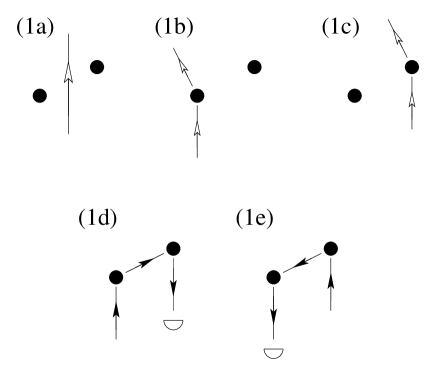
FIG. 2.: Scattering of a single photon by two distant atoms. In the coherent backscattering experiment, only the doubly scattered photon is detected, see diagrams (1d,e). Consequently, the diagrams (1a-c), with single or no scattering, describe the undetected photon.

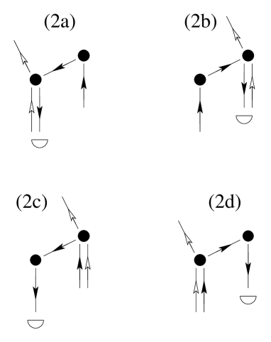
FIG. 3.: Inelastic scattering of two photons by two distant atoms. Only the doubly scattered photon (full arrows) is detected. Since the photon frequencies are changed by the inelastic scattering event at the atom where both photons meet, the amplitude of the elastic scattering event at the second atom depends on whether the inelastic scattering occurs before the elastic one (2c,d) or after (2a,b).

the photons emitted by one atom interfere with the photons emitted by the other one. Even if we average over the positions ${\bf r}_{1}$ and ${\bf r}_{2}$ of the atoms, the interference is not completely washed out. There remains an

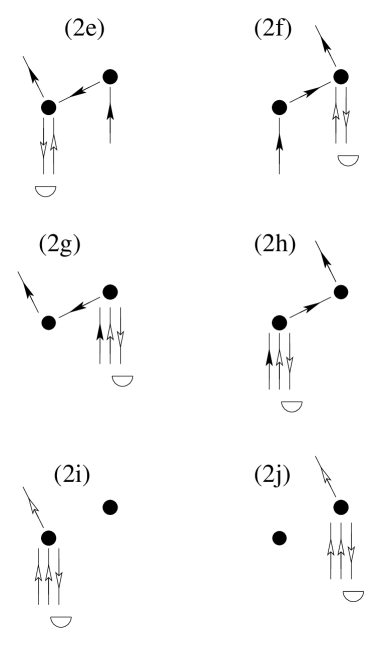
FIG. 4.: Remaining diagrams describing inelastic scattering of two photons by two atoms. In the coherent backscattering experiment, they are filtered out by using the $h\parallel h$ polarization channel (see Sec. III B), in which a singly scattered photon (open arrows) cannot be detected.

enhanced probability to detect a photon in the direction opposite to the incident wave - an effect which is known as coherent backscattering. In the case of two atoms, it arises from double scattering: in the backscattering direction, a photon scattered first by atom 1, and then by atom 2, interfers constructively with the corresponding reversed path.

In order to examine cleanly this interference effect, we therefore assume that only doubly scattered photons are detected. Experimentally, this can be realized by using circularly polarized light $\epsilon_{L}=(1,i,0)/\sqrt{2}$ (in Euclidean coordinates, where the $z$ axis is parallel to ${\bf k}_{L}$) , and detecting the scattered photons in the helicity preserving channel $\epsilon_{D}=\epsilon_{L}^{*}$. This implies $(\epsilon_{L}\cdot\epsilon_{D}^{*})=0$, i.e. no singly scattered photons can be detected in the helicity preserving polarization channel. If we look at the inelastic part of the scattering matrix, Eq. (72), assuming (without loss of generality) that the photon $|{\bf k}_{4}\epsilon_{4}\rangle$ is the detected one, this means that all terms with $(\epsilon_{1}\cdot\epsilon_{4}^{*})$ or $(\epsilon_{2}\cdot\epsilon_{4}^{*})$ are filtered out. These are the diagrams shown in Fig. 4, and only those of Fig. 3 remain. Concerning the elastic single-photon scattering, see Fig. 2 we keep the single-scattering diagrams (1a-c) to describe the undetected photon. For the sake of completeness, we will repeat in appendix B the following calculation for the case of scalar photons, where, a priori, all the diagrams shown in Figs. 2-4 contribute.

1 Elastic contribution

Let us begin with the contribution $I_{\rm el}^{(1)}$ of one-photon scattering. According to Eqs. (33,35), it is obtained by applying the electric field on the final state $|f_{1}\rangle$ of single-photon scattering. As explained above, only the diagrams (1d) and (1e) in Fig. 2 contribute. At first, we concentrate on the phase factors depending on the position of the atoms. If ${\bf k}_{L}$ is the wavevector of the incident photon, and the detector is located in the direction ${\bf k}_{D}$ (with $|{\bf k}_{D}|=|{\bf k}_{L}|$, since one-photon scattering conserves the frequency), we obtain $\exp(i{\bf r}_{1}\cdot{\bf k}_{L}-i{\bf r}_{2}\cdot{\bf k}_{D})$ for (1d) and $\exp(i{\bf r}_{2}\cdot{\bf k}_{L}-i{\bf r}_{1}\cdot{\bf k}_{D})$ for (1e). Evidently, the phases are identical if ${\bf k}_{D}=-{\bf k}_{L}$, i.e., (1d) and (1e) interfere constructively in the backscattering direction. On the other hand, if ${\bf k}_{L}\neq{\bf k}_{D}$ (more precisely: if the angle between ${\bf k}_{L}$ and ${\bf k}_{D}$ is much larger than some characteristic quantity $\theta_{C}$), the interference between (1d) and (1e) vanishes when averaging over the positions of the atoms. For simplicity, we fix the distance $r_{12}$ and average only over the angular variables of ${\bf r}_{1}-{\bf r}_{2}$. In this case, the width of the enhanced backscattering signal (which is also called ‘the cone’) is given by $\theta_{C}=1/(\omega r_{12})$. In total, we obtain both for the background intensity (known in the literature as the ‘ladder term’ $L$), and the additional intensity in backscattering direction (the ‘crossed term’ $C$) twice the result $\eta s/2$ of the single-atom case,

$$L^{(1)}=C^{(1)}={\tilde{\eta}}s,$$ (73)

apart from a modification of the prefactor

$$\tilde{\eta} = \left(\frac{3\Gamma}{4d\omega_{L}R}\right)^{2}\langle|B(\omega_{L})|^{2}|\epsilon_{L}\cdot\Delta_{12}\cdot\epsilon_{D}^{*}|^{2}\rangle_{{\bf r}_{1,2}}$$ (74)

$$= \frac{3}{8}\left(\frac{9\Gamma^{2}}{16d\omega_{L}^{2}Rr_{12}|\omega_{L}-\omega_{0}|}\right)^{2}.$$ (75)

Here, Eq. (74) implies an average over the positions of the two atoms. The polarization-dependent term $|\epsilon_{L}\cdot\Delta_{12}\cdot\epsilon_{D}^{*}|^{2}=\sin^{4}\theta/4$ is given by the angle $\theta$ between the incident laser ${\bf k}_{L}$ and the two atoms ${\bf r}_{12}={\bf r}_{1}-{\bf r}_{2}$. Then, a spherical distribution of ${\bf r}_{12}$, at fixed distance $r_{12}$, yields the result given in Eq. (75). The fact that $L^{(1)}=C^{(1)}$ can be traced back to the reciprocity symmetry [4].

Next, we examine the interference between two-photon and one-photon scattering, which gives rise to the elastic component $I_{\rm el}^{(2)}$ of the intensity in second order of $s$, see Sec. II C. According to Eq. (37), $I_{\rm el}^{(2)}$ is given by the overlap of the respective quantum states $|f_{1}\rangle$ and $|g_{1}\rangle$ of the undetected photon, which amounts to a sum over the latter’s state $|{\bf k}\epsilon\rangle$ (i.e., $\langle g_{1}|f_{1}\rangle=\sum_{{\bf k},\epsilon}\langle g_{1}|{\bf k}\epsilon\rangle\langle{\bf k}\epsilon|f_{1}\rangle$). First, we concentrate on the phase factor $\exp(-i{\bf k}\cdot{\bf r}_{1,2})$ of the undetected photon, depending on whether it is emitted by atom 1 or 2. Integrating over the angular variables $\Omega_{\bf k}$ of $\bf k$ (at fixed $|{\bf k}|=\omega_{L}$), we obtain, if $|{\bf k}\rangle$ is emitted by different atoms:

$$\int d\Omega_{\bf k}e^{\pm i{\bf k}\cdot({\bf r}_{1}-{\bf r}_{2})}=4\pi\frac{\sin(\omega_{L}r_{12})}{\omega_{L}r_{12}}\ll 1.$$ (76)

Since we have assumed $\omega_{L}r_{12}\gg 1$, the above term can be neglected. In other words, diagrams where the undetected photon is emitted by different atoms do not interfere in leading order of $1/(\omega_{L}r_{12})$. If we now select one of the four diagrams (2a-d) describing two-photon scattering, we can discard among the three one-photon diagrams (1a-c), the one where the undetected photon is scattered by the ‘wrong’ atom. The remaining two exactly give the final state of a photon scattered by a single atom, as described by Eq. (27). Concerning the detected photon of the one-photon scattering, we can choose either diagram (1d) or (1e). As already discussed above, one of them gives a contribution to the background $L$, and the other one to the enhanced backscattering signal $C$. As there are in total four diagrams (2a-d), we obtain both for $L$ and $C$ four times the result $-\eta s^{2}$ of the single-atom case:

$$L^{(2,\rm el)}=C^{(2,\rm el)}=-4{\tilde{\eta}}s^{2},$$ (77)

Note that the total elastic ladder term, Eq. (73) and Eq. (77), equals the total elastic crossed one, Eq. (73) and Eq. (77). This means interference with maximal contrast, corresponding to the maximal possible enhancement factor of two.

2 Inelastic contribution

The inelastic component $I_{\rm in}$ of the intensity, finally, arises from two-photon scattering. Here, the overlap $\langle g_{1}|g_{1}\rangle$, see Eq. 39, again implies a sum over the undetected photon, which now may have a frequency different from $\omega_{L}$. With two atoms, $|g_{1}\rangle$ is a sum of four different contributions, corresponding to the diagrams (2a-d). Correspondingly, we obtain diagonal terms ($\rm|2a|^{2},\dots,|2d|^{2}$), which contribute to the background signal, and interference terms, which may contribute to the backscattering cone, see below.

Let us examine first the diagrams (2a) and (2b), where the elastic scattering event occurs before the inelastic one. Here, the single-atom scattering amplitude is multiplied by a constant factor $B(\omega_{L})$. This means that - apart from the modification of the prefactor $\eta$ - both $\rm|2a|^{2}$ and $\rm|2b|^{2}$ give the same result as in the single-atom case, Eqs. (39,45):

$$I_{\rm II}=\frac{\tilde{\eta}}{\eta}\int d\omega P^{(in)}(\omega)={\tilde{\eta}}\frac{s^{2}}{2}.$$ (78)

In the other two cases (2c) and (2d), the frequency to be inserted in the factor $B(\omega)$, Eq. (51), equals the final frequency of the detected photon (or - equivalently - of the undetected one, since $|B(\omega)|^{2}=|B(2\omega_{L}-\omega)|^{2}$). Hence, a factor $|B(\omega)|^{2}$ must be inserted in the integral over the inelastic power spectrum, Eq. (49). The resulting integral can be easily performed, and yields:

$$I_{\rm I} = \frac{\tilde{\eta}}{\eta}\int d\omega\left|\frac{\omega_{L}-\omega_{0}}{\omega-\omega_{0}}\right|^{2}P^{(in)}(\omega)$$ (79)

$$= {\tilde{\eta}}\frac{s^{2}}{2}\left(\frac{3}{4}+\frac{\delta^{2}}{\Gamma^{2}}\right).$$ (80)

Hence, the four diagonal terms $\rm|2a|^{2},\dots,|2d|^{2}$, give the following contribution to the inelastic background intensity:

$$L^{\rm(in)}=2I_{\rm I}+2I_{\rm II}=\tilde{\eta}\left(\frac{7}{4}+\frac{\delta^{2}}{\Gamma^{2}}\right)s^{2}.$$ (81)

Note that, for $\delta=0$, the contribution from (80) is smaller than the one from (78) (by a factor $3/4$). This is due to the fact that, after the inelastic scattering event, the photon frequencies are no longer exactly on resonance, see Fig. 1(a), what reduces the cross section of the scattering by the other atom. The opposite is the case for large detuning $\delta$: here, the inelastic scattering brings one of the two photons close to the atomic resonance, see Fig. 1(b), thereby increasing the corresponding contribution to the background signal.

The inelastic component of the enhanced backscattering signal arises from the interference of (2a) with (2d), and (2b) with (2c). (Remember that every diagram interferes only with those where the undetected photon is emitted by the same atom.) As argued above, equality of the corresponding geometrical phases, and thereby full constructive interference, is guaranteed if the wavevector of the detected photon is opposite to the incident wavevector, i.e., ${\bf k}_{D}=-{\bf k}_{L}$. Obviously, this condition will not be exactly fulfilled in the presence of inelastic scattering, even in exact backscattering direction (since in general $|{\bf k}_{D}|\neq|{\bf k}_{L}|$). The difference can be neglected, however, if we assume that the atomic linewidth $\Gamma$ and the detuning $\delta=\omega_{L}-\omega_{\rm at}$, i.e. the parameters which determine the width of the power spectrum, see Fig. 1, are much smaller than the inverse of the distance $r_{12}$ between the atoms:

$$\delta,\Gamma\ll\frac{c}{r_{12}}.$$ (82)

In other words: the propagation time $r_{12}/c$ between the atoms is much smaller than the timescales associated with $\delta$ and $\Gamma$. This condition ensures a vanishing geometric phase difference, i.e. $\exp[({\bf k}_{L}+{\bf k}_{D})\cdot({\bf r}_{1}-{\bf r_{2}})]\simeq 1$, and is well fulfilled in the experiment [16]. What remains is the integration over the inelastic spectrum, taking into account the photon exchange factors $B(\omega_{L})$ or $B(\omega)$ in the cases (2a,b) or (2c,d), respectively:

$$2\int d\omega{\rm Re}\left\{\frac{\omega_{L}-\omega_{0}}{\omega-\omega_{0}}\right\}P^{\rm(in)}(\omega)=\frac{3}{4}\eta s^{2}.$$ (83)

Here, we have neglected the exponential factor $e^{i(\omega-\omega_{L})r_{12}}\simeq 1$ describing the propagation in the vacuum - the same approximation as above, see Eq. (82). From the two interfering pairs of diagrams, the inelastic contribution to the backscattering signal is obtained as twice the result of Eq. (83) with modified prefactor $\tilde{\eta}$:

$$C^{(\rm in)}=\tilde{\eta}\frac{3}{2}s^{2}.$$ (84)

Note that $C^{(\rm in)}$ is strictly smaller than the inelastic background, Eq. (81), which leads to a reduction of the backscattering enhancement factor, see below. This is consistent with the fact that two interfering diagrams, e.g. (2a) and (2d), are no more linked by the reciprocity symmetry: only diagrams with identical initial and final photon frequencies interfere with each other, whereas the reciprocity symmetry connects diagrams where initial and final frequencies are exchanged.

3 Double scattering enhancement factor

Adding all contribution, we have:

$$L=L^{(1)}+L^{(2,\rm el)}+L^{(\rm in)} = \tilde{\eta}\left(s-\frac{9}{4}s^{2}+\frac{\delta^{2}}{\Gamma^{2}}s^{2}\right)$$ (85)

$$C=C^{(1)}+C^{(2,\rm el)}+C^{(\rm in)} = \tilde{\eta}\left(s-\frac{5}{2}s^{2}\right).$$ (86)

Finally, the double scattering enhancement factor reads:

$$\alpha=\frac{L+C}{L}=\frac{8-(19-4\delta^{2}/\Gamma^{2})s}{4-(9-4\delta^{2}/\Gamma^{2})s}.$$ (87)

Remember that single scattering has been removed by the helicity-preserving polarization channel.

At this stage, it is convenient to introduce the saturation parameter on resonance:

$$s_{0}~{}=~{}\frac{2d^{2}I_{\rm in}}{\Gamma^{2}/4}~{}=\left(1+\frac{4\delta^{2}}{\Gamma^{2}}\right)s,$$ (88)

which depends only on the incident intensity $I_{\rm in}$ (and not on the detuning $\delta$). Then, Eq. (87) can be rewritten:

$$\alpha~{}=~{}\frac{2+x}{1+x},$$ (89)

with

$$x=\frac{s_{0}}{4-10s}\simeq\frac{s_{0}}{4}.$$ (90)

Here, we have used that $s$ is small - otherwise, our perturbative treatment (two-photon scattering) would be invalid. If the detuning $\delta$ is of the order of the linewidth

FIG. 5.: The enhancement factor $\alpha=(8+s_{0})/(4+s_{0})$ as a function of the incident intensity $s_{0}$, and large detuning $\delta=\omega_{L}-\omega_{\rm at}$. If $\delta$ is not large, the displayed curve is valid only up to intensities $s_{0}\ll 1+4\delta^{2}/\Gamma^{2}$, corresponding to a small saturation parameter $s\ll 1$, cf. Eq. (88).

$\Gamma$, this implies that $s_{0}$ must also be small. In this case, Eq. (89) yields:

$$\alpha\simeq 2-\frac{s_{0}}{4}.$$ (91)

In principle, however, we may choose also a large value of the detuning $\delta$, as long as we stay near-resonant, and fulfill $(\delta/\Gamma)^{2}\ll 1/(\omega r_{12})^{2}$. This means that $s_{0}$ may be large although $s$ is small, see Eq. (88). In that case, the enhancement factor is given by Eq. (89), with $x=s_{0}/4$, see Fig. 5. This equation is valid for all values of $s_{0}$ corresponding to small $s$, i.e. $s_{0}\ll 1+4\delta^{2}/\Gamma^{2}$.

It may appear surprising that the enhancement factor $\alpha$ depends only on the intensity $s_{0}$ of the incident light, see Eqs. (89,90), whereas the intensity scattered by a single atom is determined by the saturation parameter $s$, see Sec. II C. This result is related to the form of the inelastic spectrum, see Fig. 1: since one of the two photons is always close to the atomic resonance after the inelastic scattering, the asymmetry between the reversed paths (see the following section) is larger for larger initial detuning $\delta$, at a given value of $s$. Thereby, we can understand why, at a fixed $s$, the enhancement factor $\alpha$ decreases when increasing $\delta$. However, we are not aware of an intuitive explanation why the relevant parameter turns out to be $s_{0}$, and not some other, similar combination of $\delta$ and $s$.

FIG. 6.: Two reversed scattering paths, whose interference gives rise to enhanced backscattering. The left atom scatters inelastically, changing the photon frequency from $\omega_{L}$ to $\omega_{D}$. Consequently, the amplitudes of the elastic scattering event by the right atom are different for both paths, see Eqs. (92,93). This leads to a reduced contrast of the interference pattern as a function of the detection angle $\theta$, see Fig. 7.

C Interpretation: which-path information and coherence loss

In this section, we discuss the physical mechanism responsible for the reduction of the backscattering enhancement factor. As we have seen above, it originates solely from inelastic scattering. For this reason, we will only consider inelastic scattering in the following.

1 Interference between counterpropagating paths

Generally, coherent backscattering arises from constructive interference between two scattering paths where the detected photon interacts with the respective scatterers in opposite order. The maximum enhancement factor of two is obtained if every path has a counterpropagating counterpart with the same amplitude. In the case of two photons, a ‘scattering path’ in principle also specifies the final state $|{\bf k}\rangle$ of the undetected photon. As we have seen above, Eq. (76), the average over the angular variables of the undetected photon destroys interference between paths where the inelastic scattering occurs at different atoms (if the atoms are far away from each other). Consequently, if we concentrate on the detected photon, we should compare only the two reversed paths where the inelastic scattering occurs at the same atom, and the final frequency $\omega_{D}=2\omega_{L}-\omega_{\bf k}$ is the same (due to energy conservation), as shown in Fig. 6. Here, the left atom is marked as the one which scatters inelastically. Neglecting the propagation in the vacuum, see Eq. (82), the amplitudes $E_{\rm I,II}$ of the two reversed paths are obtained by multiplying the scattering amplitudes of the elastic and inelastic scattering event, Eqs. (9,16). Since the elastic scattering occurs at two different frequencies $\omega_{L}$ and $\omega_{D}$, the amplitudes are not identical:

$$E_{\rm I} = \left(\frac{1}{\omega_{D}-\omega_{0}}+\frac{1}{2\omega_{L}-\omega_{D}-\omega_{0}}\right)\frac{e^{-ikr_{\perp}\theta/2}}{\omega_{D}-\omega_{0}}$$ (92)

$$E_{\rm II} = \left(\frac{1}{\omega_{D}-\omega_{0}}+\frac{1}{2\omega_{L}-\omega_{D}-\omega_{0}}\right)\frac{e^{ikr_{\perp}\theta/2}}{\omega_{L}-\omega_{0}},$$ (93)

where $\theta$ denotes the angle between detector and backscattering direction, $r_{\perp}$ the perpendicular distance between the atoms, and prefactors not depending on $\omega_{D}$ or $\theta$ are neglected.

The asymmetry of amplitudes leads to a loss of contrast in the interference pattern:

$$|E_{\rm I}+E_{\rm II}|^{2}=|E_{\rm I}|^{2}+|E_{\rm II}|^{2}+2|E_{\rm I}||E_{\rm II}|\cos\left(\phi_{0}+kr_{\perp}\theta\right),$$ (94)

if we plot the intensity as a function of the detection angle $\theta$, see Fig. 7(a). Here, the value of the phase shift reads:

$$\tan(\phi_{0})=\frac{2\left(\delta-\epsilon\right)\Gamma}{4\delta\epsilon+\Gamma^{2}},$$ (95)

and $-\pi<\phi_{0}<\pi$, where $\epsilon=\omega_{D}-\omega_{\rm at}$ is the detuning of the detected photon. The maximum contrast, where the intensity oscillates between zero and two times the mean value as a function of $\theta$, is achieved only in the case $|E_{\rm I}|=|E_{\rm II}|$. Nevertheless, also for $|E_{\rm I}|\neq|E_{\rm II}|$, the two amplitudes interfere perfectly coherently: the contrast is as large as it can be, given that the probabilities $|E_{\rm I,II}|^{2}$ of path I and II are different. This case is analogous to a double-slit experiment performed with a perfect monochromatic plane wave, but with different slit sizes. Here also, the contrast is reduced although the wave coherence is perfectly preserved [21].

2 Second photon as a which-path detector

What we have said so far is valid if the final frequency $\omega_{D}$ is fixed. In reality, however, $\omega_{D}$ is a random variable. This implies that the ratio $E_{\rm I}/E_{\rm II}$ between the amplitudes of both paths fluctuates randomly, leading to a loss of coherence between the two paths. If we look at the interference pattern of the average intensity, integrated over $\omega_{D}$, the loss of coherence reveals itself as a reduced contrast $I_{\rm max}-I_{\rm min}<4\sqrt{I_{\rm I}I_{\rm II}}$, i.e. smaller than the maximum value for two perfectly coherent waves of intensities $I_{\rm I}$ and $I_{\rm II}$, respectively, see Eq. (94). The factor $\gamma_{\rm I,II}$ by which the contrast is reduced is called degree of coherence (see [21], p. 499-503):

$$I = \int d\omega_{D}|E_{\rm I}(\omega_{D})+E_{\rm II}(\omega_{D})|^{2}$$ (96)

$$= I_{\rm I}+I_{\rm II}+2\sqrt{I_{\rm I}I_{\rm II}}~{}\gamma_{\rm I,II}~{}\cos\left(\phi+kr_{\perp}\theta\right),$$ (97)

with $I_{\rm I}$ and $I_{\rm II}$ the average intensities of path I and II, respectively, given by Eqs. (78,80), and $\phi$ the remaining phase shift. An example is shown in Fig. 7(b). To make the loss of coherence visible, we have indicated by the arrows the contrast obtained for the same values of $I_{\rm I,II}$, but $\gamma_{\rm I,II}=1$.

An alternative physical explanation of the coherence loss can be obtained by an analogy to Young’s famous double-slit experiment. As it is well known, interference is necessarily destroyed whenever we observe which slit the particle passes through (see, e.g., [22]). If $|D_{\rm I}\rangle$ and $|D_{\rm II}\rangle$ denote the quantum states of the which-path detector corresponding to path I and II, the degree of coherence is obtained as the overlap of the normalized detector states [20]:

$$\gamma_{\rm I,II}=\frac{\left|\langle D_{\rm I}|D_{\rm II}\rangle\right|}{\sqrt{\langle D_{\rm I}|D_{\rm I}\rangle\langle D_{\rm II}|D_{\rm II}\rangle}},$$ (98)

This implies perfect coherence, $\gamma_{\rm I,II}=1$, if the paths are indistinguishable (i.e. if the detector states are identical), and total loss of coherence, $\gamma_{\rm I,II}=0$, if the paths can be distinguished with certainty (i.e. if the detector states are orthogonal).

In our case, the path detector is given by the undetected photon. Remember that its frequency is correlated to the one of the detected photon, due to conservation of energy at the inelastic scattering event. Therefore, the different dependence of the amplitudes $E_{\rm I,II}$ of path I and II on the frequency of the detected photon, see Eqs. (92,93), reflects itself in the final state of the undetected photon:

$$|D_{\rm I}\rangle = \sum_{{\bf k}\epsilon}E_{\rm I}(2\omega_{L}-\omega_{\bf k})(\epsilon_{L}\cdot\epsilon^{*})|{\bf k}\epsilon\rangle,$$ (99)

$$|D_{\rm II}\rangle = \sum_{{\bf k}\epsilon}E_{\rm II}(2\omega_{L}-\omega_{\bf k})(\epsilon_{L}\cdot\epsilon^{*})|{\bf k}\epsilon\rangle.$$ (100)

Since $|D_{\rm I}\rangle$ and $|D_{\rm II}\rangle$ are not identical, the state of the undetected photon contains information about which path the first photon has taken. This leads to a loss of coherence according to Eq. (98). Using Eqs. (92,93), we obtain:

$$\gamma_{\rm I,II} = \sqrt{\frac{9+4\delta^{2}/\Gamma^{2}}{12+16\delta^{2}/\Gamma^{2}}},$$ (101)

$$\tan(\phi) = \frac{2\delta}{3\Gamma},$$ (102)

and $-\pi<\phi<\pi$. The probabilities of the two paths, $I_{\rm I}=\langle D_{\rm I}|D_{\rm I}\rangle$ and $I_{\rm II}=\langle D_{\rm II}|D_{\rm II}\rangle$, respectively, have been calculated in the previous section, see Eqs. (78,80). Note that the phase shift, Eq. (102), vanishes for zero detuning - this can be traced back to the symmetry of the power spectrum with respect to $\omega_{\rm at}$, see Fig. 1(a), and the fact that the scattering amplitude $(\omega_{L}-\omega_{0})^{-1}=-2i/\Gamma$ is purely imaginary at resonance, $\omega_{L}=\omega_{\rm at}$.

One may wonder how the which-path information can be extracted from the second photon. In principle, this is possible, e.g., by performing a projection $|D_{\rm I}\rangle\langle D_{\rm I}|$, with possible measurement results ‘0’ and ‘1’. If we measure ‘0’, we know with certainty that path II has been taken, whereas in the case ‘1’, both paths are possible, but with increased probability of path I. Due to the rather complicated expressions of $|D_{\rm I}\rangle$ and $|D_{\rm II}\rangle$, see Eqs. (99,100), it seems rather difficult to build such a detector in practice. The simplest observation is to look at the frequency $\omega_{\bf k}=2\omega_{L}-\omega_{D}$. Since $|E_{\rm I}(\omega_{D})|^{2}$ and $|E_{\rm II}(\omega_{D})|^{2}$ depend differently on $\omega_{D}$, this observation does give some information about the path, although it does not resolve the phase dependence of $E_{\rm I}(\omega_{D})$ and $E_{\rm II}(\omega_{D})$. Nevertheless, the state of the second photon is completely determined by $\omega_{\bf k}$ (since the angular distribution is given by the polarization, independent of I or II). This implies that the which-path information can be erased by putting a spectral filter in front of the detector. Then, the measurement of the frequency gives no information (since it is always the same, determined by the filter), and, consequently, the coherence is fully restored, see Fig. 7(a).

3 Coherence between the light emitted by atom 1 and 2

At first sight, it may seem surprising that, for $\delta>0$, the maximum of the interference pattern is not found in the backscattering direction, at $\theta=0$. The reason is that we have specified the inelastically scattering atom, see Fig. 6, thereby introducing an asymmetry. However, with equal probability, the inelastic scattering may occur at the other atom, and then the interference pattern is shifted in the opposite direction. As already mentioned above, these two cases do not interfere, since they are distinguished by the undetected photon (in a similar way as the coherence between path I and II is reduced). If we add therefore both interference patterns incoherently, the new maximum is found at $\theta=0$ (as it should be), and the contrast of the interference pattern will be further reduced, by a factor $\cos(\phi)$:

$$I_{\rm tot}=\underbrace{2I_{\rm I}+2I_{\rm II}}_{\displaystyle L^{(\rm in)}}+\underbrace{4\sqrt{I_{\rm I}I_{\rm II}}~{}\gamma_{\rm I,II}\cos(\phi)}_{\displaystyle C^{(\rm in)}}~{}\cos(kr_{\perp}\theta).$$ (103)

In the backscattering direction, $\theta=0$, we recover the total intensity as a sum of a background and an enhanced backscattering term $L^{(\rm in)}$ and $C^{(\rm in)}$, which we have calculated in the previous section, see Eqs. (81,84).

What degree of coherence do we associate to the total interference pattern? Note that we are now dealing with four different diagrams, see Fig. 3, whereas (second-order) coherence is a property of two interfering waves. Therefore, before we speak of coherence, we have to specify how to divide the four diagrams into two waves. For that purpose, we consider the light emitted by atom 1 as the first wave, see diagrams (2a) and (2c), and the light by atom 2 as the second one, see diagrams (2b) and (2d). Indeed let us point out, even if it is obvious, that the total scattered electrical field is the sum of the electrical fields radiated by each atom in response to the local electrical field. This local field embodies the incident field and the field radiated by the other atom. This means that multiple scattering is taken into account. Thus, the total radiated intensity contains interference terms between the fields radiated by each atom, some of them surviving the spatial and spectral averaging in the backscattering direction. In this respect, the CBS signal probes the spatial coherence between the two radiated fields.

For reasons of symmetry, the intensities emitted by atom 1 and 2 are identical:

$$I_{1}=I_{2}=I_{\rm I}+I_{\rm II}.$$ (104)

According to the definition of the degree of coherence,

$$I_{\rm tot}=I_{1}+I_{2}+2\sqrt{I_{1}I_{2}}~{}\gamma_{1,2}~{}\cos(kr_{\perp}\theta),$$ (105)

see Eq. (97), and taking into account Eqs. (103,104), we obtain

$$\gamma_{1,2}=\gamma_{\rm I,II}\cos(\phi)\frac{2\sqrt{I_{\rm I}I_{\rm II}}}{I_{\rm I}+I_{\rm II}}.$$ (106)

On the other hand, if we compare (106) with the underbraced terms in Eq. (103), the close relation between $\gamma_{1,2}$ and the backscattering enhancement factor $\alpha^{(\rm in)}$ (considering only inelastic scattering) becomes evident:

$$\gamma_{1,2} = \frac{C^{(\rm in)}}{L^{(\rm in)}}=\alpha^{(\rm in)}-1$$ (107)

$$= \frac{6}{7+4\delta^{2}/\Gamma^{2}}.$$ (108)

Here, we have inserted the results (81,84) of the previous section. From Eq. (106), we see that the coherence $\gamma_{1,2}$ between atom 1 and 2 is reduced by the average over the power spectrum, leading to $\gamma_{\rm I,II}<1$, on the one hand, and by the random choice of atom 1 or 2 as the inelastically scattering atom, on the other one. The latter affects the coherence both due to different phases $\pm\phi$ and different amplitudes $I_{\rm I}$ and $I_{\rm II}$. For not too large values of the detuning $\delta$, the amplitude term can almost be neglected (being larger than $96\%$ for $\delta<\Gamma$), whereas the phase term $\cos(\phi)$, although strictly vanishing at $\delta=0$, gives a significant contribution if $\delta$ is of the order of $\Gamma$, see Eq. (102).

Let us note that the above interpretation in terms of a which-path experiment remains valid when adding the new pair of diagrams. Then, the detector states $|D_{\rm 1,2}\rangle$ are given by the state of the undetected photon represented by diagram $(2a)+(2c)$, on the one hand, and $(2b)+(2d)$, Fig. 3, on the other one. Similarly, we may also include the elastic component of the photodetection

FIG. 7.: Intensity of the inelastic detection signal (suitably normalized), as a function of the angle $\theta$ between detector and incident light, for detuning $\delta=\Gamma$. In (a), both the final frequency $\omega_{D}$ and the positions ${\bf r}_{12}$ of the elastically and inelastically scattering atom are fixed ($\omega_{D}=\omega_{\rm at}$ and $r_{\perp}=2r_{12}/3$), (b) shows the average over $\omega_{D}$, and (c) the average over both $\omega_{D}$ and ${\bf r}_{12}$. To make the loss of coherence due to the average over the power spectrum visible, the arrows in (b) indicate the contrast for perfect coherence, $\gamma_{\rm I,II}=1$, but same asymmetry $I_{\rm I}/I_{\rm II}$, cf. Eq. (97). The average over the positions, apart from washing out the side maxima, leads to a further loss of coherence, due to exchange of the inelastically and elastically scattering atom (see main text).

signal, where the undetected photon is described by the diagrams in Fig. 2. Furthermore, also the relation between degree of coherence, $\gamma_{12}$, and enhancement factor $\alpha$, Eq. (107), remains valid for the total signal (as it is always the case if $I_{1}=I_{2}$):

$$\gamma_{12}^{(\rm el+in)}=\frac{C}{L}=\alpha-1=\frac{4}{4+s_{0}},$$ (109)

where we have inserted Eqs. (89,90) of the previous section.

The average over the positions ${\bf r}_{1}$ and ${\bf r}_{2}$ of the atoms, finally, does not affect the intensity observed at $\theta=0$; it only reduces the side maxima, and determines the shape of the backscattering ‘cone’. As an example, Fig. 7(c) shows the result for an angular average over ${\bf r}_{2}-{\bf r}_{1}$, at fixed distance $r_{12}$, where the cone shape is described by the function $\sin(x)/x$.

Finally, we want to stress that there is no loss of coherence associated with the inelastic scattering ‘on its own’, but only in connection with the frequency filtering induced by the elastic scattering event. This can be demonstrated as follows: let us imagine that the response of the second atom is frequency-independent, i.e. $B(\omega)={\rm const}$ in Eq. (51). Then, the amplitudes of two reversed paths, see Eqs. (92,93), are identical, the undetected photon does not carry any which-path information, and we recover the enhancement factor two, even in the presence of inelastic scattering. Such a situation can be realized, e.g., by choosing atoms with different linewidths $\Gamma_{2}\gg\Gamma_{1}$, such that atom 2 cannot resolve the spectrum emitted by atom 1. In this case, a significant reduction of the enhancement factor is observed only if we increase the distance $r_{12}$ between the atoms, such that the propagation in the vacuum becomes relevant.

D Conclusion

In summary, we have presented the first calculation of coherent backscattering in the presence of saturation. For two distant atoms, with single scattering excluded, the slope of the backscattering enhancement factor as a function of the incident intensity $s_{0}$ at $s_{0}=0$ equals $-1/4$, independently of the value of the detuning. The reduction of the enhancement factor can be traced back to the following two random processes: firstly, the frequency of the photons may be changed by the inelastic scattering event, which may, secondly, occur either at the first or at the second atom. Both processes (the latter one only for nonzero detuning, see Eq. (102)) lead to a random phase shift between the doubly scattered light emitted by the first atom, on the one hand, and by the second atom, on the other one, resulting in a loss of coherence. Alternatively, the coherence loss can be explained by regarding the undetected photon as a which-path detector: its final state contains information about whether the detected photon has been emitted by the first or second atom, thereby partially destroying coherence between those paths.

Starting from the solution of our model, we can think of extending it to more general scenarios in two different directions, either increasing the number of photons, to reach higher values of the saturation parameter, or the number of atoms, to treat a disordered medium of atoms. Since the complexity of the scattering approach increases dramatically with the number of scattered particles, it may be more promising to use other methods, such as the optical Bloch equations [17], in the case of high saturation. The opposite is true for a large number of scatterers, where we can resort to known concepts from the theory of multiple scattering. An important question, which must be solved in order to interpret the results of the experiment [16], is how the average propagation of the two-photon state in the atomic medium affects the coherent backscattering signal.

A Two-atom scattering matrix

In this appendix, we calculate the scattering of two photons by two atoms. For this purpose, we use the following expansion of the evolution operator $U(t_{0},t)=\exp[-i(H_{0}+V)(t-t_{0})]$:

$$U(t_{0},t) = \sum_{n=0}^{\infty}\int_{t_{0}}^{t}dt_{1}\int_{t_{1}}^{t}dt_{2}\dots\int_{t_{n-1}}^{t}dt_{n}$$ (A2)

$$U_{0}(t_{0},t_{1})VU_{0}(t_{1},t_{2})V\dots VU_{0}(t_{n},t),$$

where $U_{0}(t_{0},t)=\exp[-iH_{0}(t-t_{0})]$ denotes the free evolution. With each interaction $V$, see Eq. (3), an atom may emit a photon, or absorb one of the two photons. The corresponding ‘paths’ connecting the initial and final two-photon state $|i\rangle=|{\bf k}_{1}\epsilon_{1},{\bf k}_{2}\epsilon_{2}\rangle$ and $|f\rangle=|{\bf k}_{3}\epsilon_{3},{\bf k}_{4}\epsilon_{4}\rangle$ can be represented diagrammatically, see Fig. 8.

FIG. 8.: Diagrams describing scattering of two photons by a single atom (Ia,b) and two atoms, (IIa,b) and (IIIa,b). The curly lines represent photons, and thin or thick lines an atom in the ground or excited state. In order to simplify the comparison between (I) and (II), we split the diagrams into a right and a left half (see main text).

Here, (Ia,b) describes the scattering of two photons by a single atom [18], and (IIa,b) and (IIIa,b) the scattering by two atoms. Let us first concentrate on (Ia,b) and (IIa,b), where the inelastic scattering event occurs before the elastic one. Note that in (IIa), we have not specified the order in which the photons are emitted or absorbed. What we mean by this is a sum over all possible orderings, as indicated in Fig. 9. As we will see below, however, the sum need not be explicitly evaluated.

FIG. 9.: Independent scattering of two photon by two different atoms. This diagram appears as a building block in (IIa) and (IIIb), Fig. 8.

Furthermore, we have selected one of the interaction operators $V$ in the expansion (A2), at which we split the diagrams into a right and left half, denoted by $U^{(l,r)}$ in the following. According to Eq. (A2), we may write:

$$U_{\rm IIa}(t_{0},t)~{}=~{}\int_{t_{0}}^{t}dt_{1}U^{(l)}_{\rm IIa}(t_{0},t_{1})VU^{(r)}_{\rm IIa}(t_{1},t),$$ (A3)

and similarly for the other three diagrams (Ia), (Ib), and (IIb). Obviously, the left half is identical in the one- and two-atom case I and II, respectively. In the right half, on the other hand, the two photons are always independent from each other, being scattered by different atoms (if at all). This means that the evolution operator is the product of the two single-photon evolution operators:

$$U_{\rm IIa}^{(r)}(t_{1},t)~{}=~{}U_{\rm II}^{(r,1)}(t_{1},t)U^{(r,2)}_{\rm a}(t_{1},t),$$ (A4)

and likewise for (Ia), (Ib), and (IIb). Note that the evolution of the first photon ($1\to 3$) depends only on (I) or (II), and not on (a) or (b), and vice versa for the second photon. Thereby, if we want to compare the one- and two-atom case, we have to consider only the two single-photon diagrams $U^{(r,1)}_{\rm I,II}$, which are illustrated in Fig. 10.

FIG. 10.: (I) Emission of a photon $|{\bf k}_{3}\epsilon_{3}\rangle$ at time $t_{1}$. (II) Photon emission and subsequent scattering by the second atom.

The first one simply describes the emission of photon $|{\bf k}_{3}\epsilon_{3}\rangle$ by an atom located at ${\bf r}_{1}$, followed by free evolution:

$$VU^{(r,1)}_{\rm I}(t_{1},t)~{}=~{}-ig(\epsilon_{1}\cdot\epsilon_{3}^{*})e^{-i{\bf k}_{3}\cdot{\bf r}_{1}}e^{-i\omega_{3}(t-t_{1})}$$ (A5)

In the second case, the photon is scattered by the other atom. Here, we have to take the sum over its intermediate state. For the calculation, it is convenient to express the time evolution in terms of the corresponding Green’s function:

$$VU^{(r,1)}_{\rm II}(t_{1},t)~{}=~{}\int_{C^{+}}\frac{dz}{2\pi i}e^{-iz(t-t_{1})}G^{(r,1)}_{\rm II}(z),$$ (A6)

where the contour $C^{+}$ runs just above the real axis, i.e., $z=x+i\epsilon$, $\epsilon>0$, from $x=+\infty$ to $-\infty$, and the Green’s function of the above diagram (II) reads:

$$G^{(r,1)}_{\rm II}(z)=\sum_{{\bf k},\epsilon}\frac{-ig^{3}(\epsilon_{1}\cdot\epsilon^{*})(\epsilon\cdot\epsilon_{3}^{*})e^{-i{\bf k}\cdot{\bf r}_{1}+i({\bf k}-{\bf k}_{3})\cdot{\bf r}_{2}}}{(z-\omega_{k})(z-\omega_{0})(z-\omega_{3})}.$$ (A7)

In the continuous limit ($L\to\infty$), the sum is replaced by an integral ($\sum_{k}=(L/2\pi)^{3}\int dk$). The result of the integral (A7), in leading order of $1/(\omega_{3}r_{12})$, reads:

$$G^{(r,1)}_{\rm II}(z)=\frac{3i\Gamma g(\epsilon_{1}\cdot\Delta_{12}\cdot\epsilon_{3}^{*})e^{-i{\bf k}_{3}\cdot{\bf r}_{2}}e^{izr_{12}}}{4\omega_{3}r_{12}(z-\omega_{0})(z-\omega_{3})}.$$ (A8)

Here, $\Delta_{12}$ denotes the projection onto the plane orthogonal to ${\bf r}_{2}-{\bf r}_{1}$. Finally, in the contour integral (A6), only the pole at $z=\omega_{3}$ contributes (if $t-t_{1}\gg 1/\Gamma$):

$$VU^{(r,1)}_{\rm II}(t_{1},t) = ig(\epsilon_{1}\cdot\Delta_{12}\cdot\epsilon_{3}^{*})e^{-i{\bf k}_{3}\cdot{\bf r}_{2}}e^{-i\omega_{3}(t-t_{1})}$$ (A10)

$$\times\frac{3\Gamma e^{i\omega_{3}r_{12}}}{4\omega_{3}r_{12}(\omega_{3}-\omega_{0})}.$$

Comparing Eqs. (A5,A10), we see that the contribution to the two-atom scattering matrix represented by (IIa,b) is given by the one-atom matrix $S_{\rm I}$, times a correction of the geometrical phase and the polarization, times the photon exchange factor $B(\omega_{3})$, see Eq. (51).

$$\langle{\bf k}_{3}\epsilon_{3},{\bf k}_{4}\epsilon_{4}|S_{\rm II}|{\bf k}_{1}\epsilon_{1},{\bf k}_{2}\epsilon_{2}\rangle = \langle{\bf k}_{3}\epsilon_{3},{\bf k}_{4}\epsilon_{4}|S_{\rm I}|{\bf k}_{1}\epsilon_{1},{\bf k}_{2}\epsilon_{2}\rangle$$ (A12)

$$\!\!\!\!\!\!\!\!\!\!\!\!\!\!\!\!\!\!\!\!\!\!\!\!\!\!\!\!\!\!\!\!\times e^{i{\bf k}_{3}\cdot({\bf r}_{1}-{\bf r}_{2})}\frac{(\epsilon_{1}\cdot\Delta_{12}\cdot\epsilon_{3}^{*})}{(\epsilon_{1}\cdot\epsilon_{3}^{*})}B(\omega_{3}).$$

What remains is the contribution, where the elastic scattering occurs before the inelastic one, represented by diagrams (IIIa,b) in Fig. 8. The calculation can be repeated in almost the same way as above, or simply by noting that (IIIa,b) is related to (IIa,b) through time reversal, and the result is:

$$\langle{\bf k}_{3}\epsilon_{3},{\bf k}_{4}\epsilon_{4}|S_{\rm III}|{\bf k}_{1}\epsilon_{1},{\bf k}_{2}\epsilon_{2}\rangle = \langle{\bf k}_{3}\epsilon_{3},{\bf k}_{4}\epsilon_{4}|S_{\rm I}|{\bf k}_{1}\epsilon_{1},{\bf k}_{2}\epsilon_{2}\rangle$$ (A14)

$$\!\!\!\!\!\!\!\!\!\!\!\!\!\!\!\!\!\!\!\!\!\!\!\!\!\!\!\!\!\!\!\!\times e^{-i{\bf k}_{1}\cdot({\bf r}_{1}-{\bf r}_{2})}\frac{(\epsilon_{1}\cdot\Delta_{12}\cdot\epsilon_{3}^{*})}{(\epsilon_{1}\cdot\epsilon_{3}^{*})}B(\omega_{1}).$$

Here, the photon exchange factor $B(\omega)$ is evaluated at the frequency of the initial photon. The total scattering matrix is now readily obtained by adding $S_{\rm II}$ and $S_{\rm III}$, and also including the diagrams where the two atoms and/or the two photons are exchanged.

B The scalar case

In this appendix, we calculate the photodetection signal for scalar photons. Although they are not suited for coherent backscattering, since single scattering cannot be excluded, the solution will be useful for a future comparison with the results obtained from the optical Bloch equations, which can be solved much more easily in the scalar case.

As in the vectorial case, we consider contributions to the detection signal up to second order in $1/(\omega_{L}r_{12})$. We neglect those terms whose order in $1/(\omega_{L}r_{12})$ is changed by the angular average over ${\bf r}_{12}$. Furthermore, we consider only contributions which do not oscillate rapidly as a function of $r_{12}$, i.e. which survive an average over $r_{12}$ over one wavelength.

Firstly, since the two atoms may scatter independently from each other, we obtain two times the single-atom result, see Eqs. (44,45):

$$L^{({\rm el},0)} = \eta_{s}(s-2s^{2}),$$ (B1)

$$L^{({\rm in},0)} = \eta_{s}s^{2},$$ (B2)

which contributes to the background intensity $L$. Here we have to take into account that the lifetime $\Gamma$, and the prefactor $\eta$, are different in the scalar and vectorial case, respectively. Instead of Eqs. (5,46), the following expressions hold for scalar photons:

$$\Gamma_{s} = \frac{d^{2}\omega_{\rm at}^{3}}{2\pi\epsilon_{0}}$$ (B3)

$$\eta_{s} = \left(\frac{\Gamma_{s}}{2d\omega_{L}R}\right)^{2}.$$ (B4)

Next, we consider the cases where one photon is exchanged between the two atoms. These contribute to the detection signal in second order of $1/(\omega_{L}r_{12})$. Concerning one-photon scattering, only the diagrams (1d,e), Fig. 2, are relevant, and we obtain the same result as for the $h\parallel h$ channel in the vectorial case, see Eq. (73):

$$L^{({\rm el},1)}=C^{({\rm el},1)}=\eta_{s}|B|^{2}s,$$ (B5)

but with modified ‘photon exchange factor’

$$B=\frac{\Gamma}{2\omega_{L}r_{12}(\omega_{L}-\omega_{0})},$$ (B6)

compare Eq. (51).

The elastic contribution quadratic in $s$ arises from interference of two-photon and one-photon scattering. Let us first look at diagram (2a). As before in the $h\parallel h$ channel, it interferes with (1a+1b) for the undetected photon, and (1d) or (1e) for the detected photon, giving rise to $-\eta_{s}|B|^{2}s^{2}$ in background $L$ and the cone $C$, respectively. Including single scattering, we obtain a new contribution: the detected photon may be singly scattered (1b), and the undetected photon either doubly scattered (1e), or singly-scattered by the other atom (1c). Here, the state (1e+1c), of the undetected photon exactly corresponds to the state (1a+1b), in the previous case. Consequently, we obtain another term $-\eta_{s}|B|^{2}s^{2}$ in the background.

With diagram (2b), the above considerations can be repeated in almost the same way. The difference from (2a) is only that the detected photon propagates in the opposite direction. Consequently, we obtain a new term $-\eta_{s}|B|^{2}s^{2}$ in the cone $C$, instead of the background $L$.

Diagram (2e) is identical to diagram (2a), since we cannot distinguish between singly or doubly scattered photons (open or full arrows in Figs. 2-4) in the scalar case. (2c), (2d), and (2f), finally, are obtained by exchanging the atoms. Adding all contributions mentioned above, we get:

$$L^{(\rm el,2)} = -10\eta_{s}|B|^{2}s^{2}$$ (B7)

$$C^{(\rm el,2)} = -8\eta_{s}|B|^{2}s^{2}.$$ (B8)

As for the inelastic component, we only have to include the new diagrams (2e,f), which - as already mentioned above - are identical to (2a,b). Hence, the background contribution $2I_{\rm I}$, see Eq. (80), is multiplied by a factor $4$, and the backscattering cone, Eq. (84), by a factor $2$. We obtain:

$$L^{\rm(in,2)} = 8I_{\rm I}+2I_{\rm II}=\left(\frac{19}{4}+\frac{\delta^{2}}{\Gamma^{2}}\right)~{}\eta_{s}|B|^{2}s^{2}$$ (B9)

$$C^{\rm(in,2)} = 3\eta_{s}|B|^{2}s^{2}.$$ (B10)

What we have not taken into account so far is interference between two diagrams where the undetected photon is emitted by different atoms. According to Eq. (76), the angular integral over the undetected photon then yields $\sin(\omega r_{12})/(\omega r_{12})$. Hence, if one of the two diagrams contains a photon exchange, we obtain a contribution proportional to $|B|^{2}$. However, it can be shown that these contributions are exactly canceled by other contributions originating from the diagrams (2g,h), which also have been neglected so far. For example, the interference of (2g) with (1c) for the detected photon and (1c+1e) for the undetected one is canceled by the interference of (2j) with (1c) for the detected photon and (1e) for the undetected one. Similarly, the term $\rm|2g|^{2}$ is canceled by the interference of (2g) with (2j). The underlying reason for all these cancellations is that what the undetected photon does after the inelastic scattering is irrelevant. We are only interested in its norm, which is not changed by subsequent scattering events (due to energy conservation). Hence, the final result is given by Eqs. (B1-B10).

REFERENCES

- [1] Y. Kuga and A. Ishimaru, J. Opt. Soc. Am. A 1, 831 (1984).
- [2] M. P. van Albada and A. Lagendijk, Phys. Rev. Lett. 55, 2692 (1985).
- [3] P.E. Wolf and G. Maret, Phys. Rev. Lett. 55, 2696 (1985).
- [4] B.A. van Tiggelen and R. Maynard, in Wave Propagation in Complex Media, edited by G. Papanicolaou, IMA (Springer, Berlin 1997).
- [5] A.A. Chabanov, M. Stoytchev, and A.Z. Genack, Nature 404, 850 (2000).
- [6] D. S. Wiersma, P. Bartolini, A. Lagendijk, and R. Righini, Nature 390, 671 (1997).
- [7] F. Scheffold, R. Lenke, R. Tweer, and G. Maret, Nature 398, 207 (1999).
- [8] D. S. Wiersma, J.G. Rivas, P. Bartolini, A. Lagendijk, and R. Righini, Nature 398, 207 (1999).
- [9] G. Labeyrie, E. Vaujour, C. A. Müller, D. Delande, C. Miniatura, D. Wilkowski, and R. Kaiser, Phys. Rev. Lett. 91, 223904 (2003).
- [10] D. Wilkowski et al., Physica B 328, 157 (2003).
- [11] C. A. Müller, T. Jonckheere, C. Miniatura, and D. Delande, Phys. Rev. A 64, 053804 (2001).
- [12] C. A. Müller and C. Miniatura, J. Phys. A 35, 10163 (2002).
- [13] G. Labeyrie, F. de Tomasi, J.-C. Bernard, C. A. Müller, C. Miniatura, and R. Kaiser, Phys. Rev. Lett. 83, 5266 (1999).
- [14] T. Jonckheere, C.A. Müller, R. Kaiser, C. Miniatura and D. Delande, Phys. Rev. Lett. 85, 4269 (2000).
- [15] Y. Bidel et. al., Phys. Rev. Lett. 88, 203902 (2002).
- [16] T. Chanelière, D. Wilkowski, Y. Bidel, R. Kaiser, and Ch. Miniatura, ccsd-00000623 (2003).
- [17] C. Cohen-Tannoudji, J. Dupont-Roc, and G. Grynberg, Atom-Photon Interactions (Wiley, New York, 1992).
- [18] J. Dalibard and S. Reynaud, Journal de Physique 12, 1337 (1983).
- [19] B.R. Mollow, Phys. Rev. 188, 1969 (1969).
- [20] S.M. Tan and D.F. Walls, Phys. Rev. A 47, 4663 (1993).
- [21] M. Born and E. Wolf, Principles of Optics, Sixth Edition (Pergamon Press, Oxford, 1980).
- [22] T. Pfau, S. Spälter, Ch. Kurtsiefer, C.R. Ekstrom, and J. Mlynek, Phys. Rev. Lett. 73, 1223 (1994).