Regularization of the Coulomb scattering problem

Abstract

Exact solutions of the Schrödinger equation for the Coulomb potential are used in the scope of both stationary and time-dependent scattering theories in order to find the parameters which define regularization of the Rutherford cross-section when the scattering angle tends to zero but the distance r from the center remains fixed. Angular distribution of the particles scattered in the Coulomb field is investigated on the rather large but finite distance r from the center. It is shown that the standard asymptotic representation of the wave functions is not available in the case when small scattering angles are considered. Unitary property of the scattering matrix is analyzed and the ”optical” theorem for this case is discussed. The total and transport cross-sections for scattering of the particle by the Coulomb center proved to be finite values and are calculated in the analytical form. It is shown that the considered effects can be essential for the observed characteristics of the transport processes in semiconductors which are defined by the electron and hole scattering in the fields of the charged impurity centers.

PACS: 03.60.Nk, 03.80.+r, 34.80.-i
Keywords: nonrelativistic scattering, Coulomb potential, cross-section, regularization

I Introduction

Scattering of non-relativistic charged particles by the Coulomb center is one of the canonical problems both in classical and quantum mechanics which is known as the Rutherford problem. It is the standard point of view that the differential cross-section $d\sigma(\theta)$ of the particle scattering to the solid angle $d\Omega$ has the same form in the both cases (for example, Refs. landau1 , newton )

$$d\sigma(\theta)=\sigma(\theta)d\Omega=(\frac{\alpha}{2mv^{2}})^{2}\frac{d\Omega}{\sin^{4}\theta/2}.$$ (1)

Here m and $v$ are the particle mass and velocity correspondingly, parameter $\alpha$ defines the amplitude of the Coulomb potential $U(r)=\alpha/r$.

So, the main measured characteristic of the scattering process in the Coulomb field has the non-integrable singularity in the limit $\theta\rightarrow 0$ (in quantum theory the singularity exists also in the scattering amplitude). Fortunately, this singularity doesn’t lead to any problem when describing of the most real experiments because particles are scattered by the systems with zero total charge. In this case the singularities conditioned by the scattering centers of opposite signs are compensated and the cross-section proves to be regular in the entire angular range. Nevertheless, there are some physical systems where one should consider the problem of regularization when calculating such integral scattering characteristics as the total $\sigma_{tot}$ and transport $\sigma_{tr}$ cross-sections

$$\sigma_{tot}=\int d\sigma(\theta),\quad\sigma_{tr}=\int(1-\cos\theta)d\sigma(\theta).$$ (2)

As for example, we can mention calculation of the characteristics of kinetic processes in plasma and impurity semiconductors or collisions of the charged particles in beams. In such cases one should introduce some phenomenological parameter $\theta_{min}$ for cutting off the cross-section (1) with angles $\theta<\theta_{min}$. This parameter can be defined by various physical reasons. Particularly, in the framework of the classical mechanics the small angle scattering is defined by the particles with large impact parameter landau2 connected with a long range character of the Coulomb potential. Therefore, the small angle cone can be excluded from the consideration because of finite transversal width $a$ of the incident beam with $\theta_{min}\sim a/r$ sing .

Another approaches are used when the mobility of the charge carriers is calculated in the impurity semiconductors. The models of Brooks-Herring herring and Conwell-Weisskopf conwell are mostly used for this problem at present. These models correspond to different ways for estimation of the parameter $\theta_{min}$ connected with screening of the Coulomb potential. However, such estimations have only qualitative character and some additional phenomenological parameter should be introduced for more precise description of the mobility as it was shown recently in the paper poklonskii . Accurate calculation of the integral values characterizing the charge carrier scattering by impurities is actual because of high accuracy of measurement of these values in real semiconductors (for example, semiconducter ). Solution of this problem is of great interest also for analysis of the electron transport in nanostructures such as quantum wires wire , superlattices and films film , nanotubes tube .

Regularization problem for the Coulomb cross-section is essentially more principal in the framework of the quantum theory. The matter is that the exact wave function for the states of the continuous spectrum is well known landau1 and it has no any singularity even in the case of the plane incident wave which corresponds to the beam with the infinite transversal width. It should mean that the singularity of the scattering amplitude is not intrinsic feature of the Coulomb system in the scope of quantum mechanical description. Possibly, it could be conditioned by not completely adequate interpretation of the asymptotic behavior of the wave function in this case. One can expect that some characteristic, or ”kinematical”, regularization parameter $\theta_{0}$ should exist which doesn’t connect with the initial state of the system unlike the value $\theta_{min}$. In general case the regularized cross-section should depend on both parameters.

It is essentially to emphasize that some specific characteristics of the Coulomb scattering problem have been widely discussed in monographs and textbooks. As for example, it was shown in the book sing that the connection between the impact parameter and scattering angle becomes indefinite in the case of $\theta=0$, therefore the scattering cross-section for zero angle can’t be calculated in classical dynamics. It is also well known that long-range character of the Coulomb potential leads to the logarithmic distortion of phase in the asymptotic form of the wave function (for example landau1 ). However, the problem of the cross-section regularization has not been considered in these discussions.

This question was analyzed for the first time in our paper 1971 . It was shown that the standard asymptotic representation of the wave function was not actually formed in the range of small angles when considering the scattering processes by the long-range potentials ($U(r)\sim 1/r^{s};s\leq 3$). In the result the canonical definition of the scattering amplitude proved to be unavailable. Born approximation over the potential $U(r)$ and the non-stationary collision theory goldberger were used in our work 1971 in order to calculate the scattering cross-section without any singularities. We can also mention several papers ( zack and references therein) where it was shown that the interference between incident and scattered waves changed the asymptotic form of the wave function and could be essential in real experimental conditions even in the case of some short-range potentials.

In the present paper we consider the non-asymptotic analysis of the observed characteristics for the non-relativistic Coulomb scattering problem out of the framework of the perturbation theory. We use the exact solutions of the Schrödinger equation in order to answer the following questions: 1)which ”intrinsic” kinematical parameter defines regularization of the Rutherford cross-section in the framework of the stationary scattering theory; 2) how does this regularization depend on ”external” parameters such as the transversal width of the incidence wave packet or effective cutting off of the potential; 3) which way can one calculate non-asymptotic values for the integral scattering characteristics $\sigma_{tot},\sigma_{tr}$; 4)what is the analog of the ”optical” theorem $4\pi Imf(0)=k\sigma_{tot}$ landau1 , newton in the case of the Coulomb potential? It seems to us that the answers for these questions have the important methodical value for understanding the scattering processes in the field of long-range potentials but have not been discussed earlier. Besides, these results can be also essential for some applications such as the above-mentioned transport processes in the semiconductors with the charged impurities.

The paper is organized as follows. In Sec. 2 the differential scattering cross-section is defined without asymptotic representation of the wave functions and the kinematical regularization parameter is found for the Rutherford problem. The most important integral characteristics of the scattering problem are calculated in Sec.3. In Sec.4 the scattering operator and the conservation of the total flux are analyzed. The time-dependent consideration of the collision process is discussed in Sec. 5 and influence of the incident beam parameters and screening of the potential to the observed scattering characteristics is estimated. The scattering characteristics of the carriers in non-degenerated semiconductors with the charged impurities are calculated in Sec. 6 and the results are compared with the experimental values of the carrier mobility in real systems.

II Non-asymptotic calculation of the differential cross-section for the Coulomb scattering

Let us remind the standard definitions of the scattering theory in the stationary quantum mechanics. It is well known landau1 , that in this case the wave functions of the continuous spectrum $\psi_{\vec{k}}(\vec{r})$ should be found as the solutions of the Schrödinger equation

$$[-\frac{\hbar^{2}}{2m}(\Delta+k^{2})+U(\vec{r})]\psi_{\vec{k}}(\vec{r})=0,$$ (3)

with the following asymptotic boundary conditions (Fig.1 shows all necessary notations).

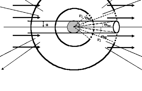
Figure 1: Sketch of the scattering process in the stationary case.

$$\psi_{\vec{k}}(\vec{r})\sim e^{i\vec{k}\vec{r}},\quad\vec{k}\vec{r}\rightarrow-\infty;$$ (4)

$$\psi_{\vec{k}}(\vec{r})\sim e^{i\vec{k}\vec{r}}+f(\theta)\frac{e^{ikr}}{r},\quad r\gg R.$$ (5)

Here $\vec{k}$ is the wave vector; the value R defines characteristic radius of the potential action with the center point $r=0$ ($R\rightarrow\infty$ in the case of the Coulomb field); the wave function is supposed to be normalized to one particle, so that the flux density in the incident state is:

$$\vec{j}=\frac{\hbar}{2im}[\psi_{\vec{k}}(\vec{r})^{*}\nabla\psi_{\vec{k}}(\vec{r})-\psi_{\vec{k}}(\vec{r})\nabla\psi_{\vec{k}}(\vec{r})^{*}]\simeq\frac{\hbar}{m}\vec{k}\equiv\vec{j}_{0},\quad\vec{k}\vec{r}\rightarrow-\infty;$$ (6)

The flux density in the asymptotic state (5) is divided on two components:

$$\vec{j}=j_{l}\frac{\vec{k}}{k}+j_{sc}\frac{\vec{r}}{r},\quad r\gg R.$$ (7)

One of them $j_{l}$ (longitudinal component) corresponds to the particles passed through the field without interaction and the second one $j_{sc}$ (radial component) describes the scattered particles. It leads to the standard definition of the cross-section:

$$d\sigma(\theta)=\frac{j_{sc}}{j_{0}}r^{2}d\Omega;$$

$$\sigma(\theta)=|f(\theta)|^{2}.$$ (8)

It should be noted that the longitudinal flux is also changed $j_{l}<j_{0}$, and its decrease is defined by the total scattering cross-section in accordance with the ”optical” theorem landau1 .

Evidently, that the definition (II) is based essentially on the asymptotic regime (5) for the wave function in the observation point r. Accordingly to the terminology used in radio-physics and optics (for example, born ), it means that the particle should go out of the ”near” zone, where the action of the potential is still essential, and pass to the ”far”, or ”wave”, zone. The boundary between these zones is defined by the condition that the interference between incident and scattered waves becomes negligible that is the difference between their phases satisfies the inequality

$$kr-\vec{k}\vec{r}=2kr\sin^{2}(\theta/2)>1;$$

$$\theta>\theta_{0}\equiv\sqrt{\frac{2}{kr}}.$$ (9)

We suppose further that for all real collisions the condition $kr\gg 1$ is fulfilled.

It is clear that the boundary of the ”wave” zone depends both on the distance r from the center and the scattering angle $\theta$ (Fig.1). It means that in general case there is a part of the particle flux which can not be described by the asymptotic wave function (5) even for rather large distance r. Certainly, that this property does not depend on the radius of the potential auction. However, the question is: what is the contribution of these particles to the integral scattering process? When the distance from the center r is fixed, the number of particles scattered to the ”near” zone $\theta<\theta_{0}$ can be estimated as

$$N_{dif}\simeq j_{0}\sigma(0)\theta^{2}_{0}\sim\frac{j_{0}\sigma(0)}{kr},$$ (10)

The cross-section $\sigma(0)$ is restricted for the potentials with the finite action radius R, therefore the $N_{dif}$ decreases quickly at the large distance. It means that the contribution of these particles to the observed scattering characteristics is negligible for the most real experiments. The detailed analysis of the ”near” and ”wave” zone formation for the scattering problem with the short-range potential has been recently considered in the paper zack .

The picture changes fundamentally in the case of the long-range potential $(R\rightarrow\infty)$ . The value $N_{dif}$ can even increase with the distance and its contribution to the formation of the scattering flux can be essential. Particularly, the analogous estimation in the case of the Coulomb field leads

$$N_{dif}\gg j_{0}(\frac{\alpha}{mv^{2}})^{2}\frac{4}{\theta^{2}_{0}}\sim kr.$$ (11)

It means that the asymptotic boundary condition (5) is not available in the entire range of the scattering angles and the nonasymptotic expression for the wave function should be used in the case of small angles. It is important to stress that this circumstance does not connect with the width of incident beam and defines by the characteristic feature of the potential itself.

So, the considered regularization problem for the Rutherford cross-section in the scope of the stationary scattering theory is reduced to the analysis of the space flux distribution on the basis of the well known exact solution of the equation (3) with the potential $U(r)=Ze^{2}/r$ but without handling to the asymptotic representation of the wave function.

We will use the following form of the normalized wave function landau1

$$\psi_{\vec{k}}(\vec{r})=Ne^{i\vec{k}\vec{r}}F[\pm i\xi,1,i(kr-\vec{k}\vec{r})];\quad N=e^{\pm\frac{\pi}{2}\xi}\Gamma(1\mp i\xi);$$

$$\xi=\frac{\alpha}{\hbar v};\quad\alpha=Ze^{2};\quad v=\frac{\hbar k}{m},$$ (12)

where $F(a,b,t)$ is the confluent hypergeometric function; $\Gamma(t)$ is the Gamma - function; the upper sign in the formulas corresponds to the attraction field and the lower one corresponds to the repulsion potential.

Let us show that the flux density in the formula (6) calculated with the exact wave function can also be divided by two components in accordance with the formula (7) as it was in the asymptotic regime . For this purpose one can use the following representation of the function F as the superposition of two confluent hypergeometric functions of the 3-rd genus $U_{1,2}(a,b,t)$ mors

$$F(\pm i\xi,1,iz)=\frac{1}{\Gamma(\pm i\xi)}U_{1}(\pm i\xi,1,iz)+\frac{1}{\Gamma(1\mp i\xi)}U_{2}(\pm i\xi,1,iz);$$

$$U_{1}(\pm i\xi,1,iz)=(z)^{\pm i\xi}\frac{e^{iz}}{\Gamma(1\mp i\xi)}e^{\mp\pi\xi}G_{1}(\pm i\xi,iz),$$

$$G_{1}(\pm i\xi,iz)=\int_{0}^{\infty}e^{-u}u^{\mp i\xi}(1-\frac{u}{iz})^{\pm i\xi}\frac{du}{iz-u};$$

$$U_{2}(\pm i\xi,1,iz)=(z)^{\mp i\xi}\frac{1}{\Gamma(\pm i\xi)}e^{\mp\pi\xi}G_{2}(\pm i\xi,iz),$$

$$G_{2}(\pm i\xi,iz)=\int_{0}^{\infty}e^{-u}u^{\pm i\xi-1}(1+\frac{u}{iz})^{\mp i\xi}du;$$

$$z=(kr-\vec{k}\vec{r})=kr(1-\cos\theta).$$ (13)

Let us also mention the connection between these functions and the confluent hypergeometric functions of the 2-nd genus $U(a,b,t)$ nikiforov

$$U_{1}(a,b,t)=U(b-a,b,-t)e^{t}e^{\pm i\pi(a-b)},$$

$$U_{2}(a,b,t)=U(a,b,t)e^{\pm ia\pi},$$

$$U(a,b,t)=\frac{1}{\Gamma(a)}\int_{0}^{\infty}e^{-tu}u^{a-1}(1+u)^{b-a-1}du;.$$ (14)

When the Rutherford cross-section is calculated by means of the standard definition this representation permits one to find the asymptotic form of the wave function in the limit $z\gg 1$ landau1 . This case corresponds to the ”wave” zone when the function $U_{1}$ transforms to the spherical wave and the function $U_{2}$ tends to the plane wave. However, both these functions are well defined also in the ”near” zone ($z<1$) when they can be calculated by means of the following serieses mors :

$$U_{1}(\pm i\xi,1,iz)=\frac{1}{2}\Gamma(\pm i\xi)\{F(\pm i\xi,1,iz)+$$

$$\frac{e^{\mp 2\pi\xi}-1}{2\pi i}[[2\ln(iz)\mp i\pi\coth(\pi\xi)-i\pi+2\psi(\pm i\xi)]F(\pm i\xi,1,iz)+$$

$$2\sum_{m=1}^{\infty}\frac{\Gamma(m\pm i\xi)}{\Gamma(\pm i\xi)(m!)^{2}}[\psi(m\pm i\xi)-\psi(\pm i\xi)+2\psi(1)-2\psi(m+1)](iz)^{m}]\};$$

$$U_{2}(\pm i\xi,1,iz)=\frac{1}{2}\Gamma(1\mp i\xi)\{F(\pm i\xi,1,iz)-$$

$$\frac{e^{\mp 2\pi\xi}-1}{2\pi i}[[2\ln(iz)\mp i\pi\coth(\pi\xi)-i\pi+2\psi(\pm i\xi)]F(\pm i\xi,1,iz)+$$

$$2\sum_{m=1}^{\infty}\frac{\Gamma(m\pm i\xi)}{\Gamma(\pm i\xi)(m!)^{2}}[\psi(m\pm i\xi)-\psi(\pm i\xi)+2\psi(1)-2\psi(m+1)](iz)^{m}]\},$$ (15)

where $\psi(t)$ is the logarithmic derivative of the Gamma-function.

When the representation (II) is used in the formula (6) one should take into account only the derivatives from the exponents because the conditions $kr\gg 1;\ z\sim 1$ supposed to be fulfilled. As for example,

$$-i(\frac{\vec{r}}{r}\vec{\nabla})[e^{ikr}G_{1}(iz)]=e^{ikr}[kG_{1}+\frac{z}{r}G^{\prime}_{1}(iz)]\simeq e^{ikr}kG_{1}[1+O(\frac{1}{kr})].$$

This representation permits one to find the scattering flux $j_{sc}$ directed to the observation point along the vector $\vec{r}$ without use of the asymptotic form (5) of the wave function. In the result the scattering cross-section can be defined in the entire range of the angles $\theta$ in the following form:

$$\sigma_{1}(\theta)d\theta=\sin\theta r^{2}\int_{0}^{2\pi}d\varphi\frac{j_{sc}}{j_{0}}d\theta=$$

$$2\xi\sinh(\pi\xi)e^{\mp\pi\xi}|G_{1}(\pm i\xi,iz)|^{2}r^{2}\sin\theta d\theta.$$ (16)

One can see that the differential cross-section $\sigma_{1}(\theta)$ is finite for any angle in spite the function $G_{1}(\pm i\xi,iz)$ has the logarithmic singularity at zero angle as it follows from the equation (II). But this value depends on the distance between the center and observation point by non-trivial way because of long-range action of the potential field to the particle. The result of this action at small angles (”near” zone) does not reduce to varying the phase of the scattering amplitude as it is takes place for the asymptotic range of angles (”wave” zone)landau1 .

If one considers behavior of the function $G_{1}(\pm i\xi,iz)$ in dependence on the scattering angle the ”kinematical” parameter $\theta_{0}$ for regularization of the Rutherford cross-section can be introduced by the natural way. Actually, the asymptotic range of angles corresponding to the ”wave” zone is defined by the condition

$$z=kr-\vec{k}\vec{r}\simeq\frac{1}{2}kr\theta^{2}\gg 1;$$

$$\theta\gg\theta_{0}=\sqrt{\frac{2}{kr}}\ll 1;\quad x\gg 1;$$

$$x=\frac{\theta}{\theta_{0}};\quad z\simeq x^{2}.$$ (17)

Here the dimensionless value x is introduced as the convenient variable for the angles compared with the width of the ”near” zone. Certainly, in the range of $x\gg 1$ the standard asymptotic representation of the integral in the definition of the function $G_{1}(\pm i\xi,iz)$ leads to the result corresponding to the formula (1) with new variable

$$\sigma_{1}(\theta)\simeq 2\pi(\frac{\xi}{k})^{2}\frac{\sqrt{2}(kr)^{3/2}}{x^{3}}=8\pi(\frac{\alpha}{mv^{2}})^{2}\frac{1}{\theta^{3}};\quad x\gg 1.$$ (18)

It is well known that the interference between the scattering flux and the flux directed along the initial velocity of the particle does not take into account in scope of any quantum scattering theory based on the solutions of the stationary Schrödinger equation landau1 . So, in order to use the formula (II) in the range $x<1$ corresponding to the ”near” zone, one should compare it with the angle width of the zone where the above mentioned interference is still essential. It is clear that the angle width of such ”interference” zone does not depend on the dynamics of the interaction between the particle and field. It is defined only by the transversal width $a$ of the incident particle wave packet (Fig.1). One can estimate the angle width $\theta_{int}$ of the ”interference” zone as follows

$$\theta_{int}\simeq\frac{a}{r}.$$ (19)

It means that one can consider the scattering flux in the near zone and at the same time neglect by its interference with the incident beam if the following conditions are fulfilled

$$\theta_{int}<\theta<\theta_{0}=\sqrt{\frac{2}{kr}};\quad\frac{ka^{2}}{r}\ll 1.$$ (20)

These inequalities are satisfied in the case of rather large $r$ as it usually supposed in the scattering theory. More accurate analysis of this factor will be considered below (Sec.3) in the framework of the time-dependent theory of collisions goldberger . But one can estimate just now the contribution of the ”interference” zone to the integral scattering characteristics which are finite values in our consideration unlike the asymptotic analysis. As for example, the ratio of the particle flux scattered at the ”interference” and ”near” zones can be estimated as

$$\delta=\frac{j_{int}}{j_{dif}}\simeq\int_{0}^{\theta_{int}}\sigma_{1}(\theta)d\theta/\int_{0}^{\theta_{0}}\sigma_{1}(\theta)d\theta\simeq\frac{ka^{2}}{2r}\ll 1.$$ (21)

It remains small under standard conditions of the collision theory goldberger and one can analyze distribution of the flux density in the ”near” zone neglecting its interference with the incident flux. It permits one to find the leading terms of the differential scattering cross-section at small angles using the series (II)

$$\sigma_{1}(\theta)\simeq 8\sqrt{2}\xi e^{\mp\pi\xi}\sinh(\pi\xi)x(\ln x)^{2}\frac{r^{3/2}}{\sqrt{k}}.$$ (22)

Fig.2 compares the accurate and asymptotic scattered fluxes for various values of the variable $x$ and parameter $\xi$. It is interesting to pay one’s attention to the essentially different behavior of the nonasymptotic flux in ”near” zone for scattering by the attractive and repulsive centers in contrast to the Rutherford cross-section (1) which is independent of the potential sign for any value $\xi$. One can see that the regularized differential cross-section (II) in the ”near” zone is essentially non-invariant relatively to the sign of the charge if the parameter $\xi\geq 1$. It should be noted that the effect of slightly different interaction of the charge carriers with the impurities of different signs is well known in the semiconductor physics. It is usually considered there by means of the Friedel sum rule fridel using the partial expansion of scattering amplitude in the series of orbital momenta.

As it follows from Eq. (22), the scattering flux in the case of attractive potential varies rather slowly with increase of the parameter $\xi$, but it grows exponentially in the case of repulsion. Certainly, such behavior of the cross-section takes place only in the narrow angle domain (20) and compensates the exponential decrease of the flux just along the line $\theta=0$ which is well known for the repulsive potential landau1

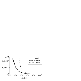
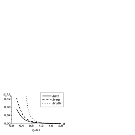
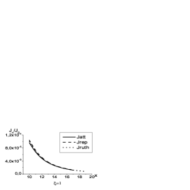
Figure 2: Ratio of the scattered flux $J_{n}$ to the density of the incident flux $J_{0}$. Solid line - the case of attraction $J_{att}$, dashed line - the case of repulsion $J_{rep}$, dotted line - the Rutherford flux $J_{ruth}$.

III Integral characteristics for the Coulomb scattering problem

Let us now calculate the integral scattering characteristics for the considered problem. In accordance with Eq. (II) the nonasymptotic expression for the total cross-section is defined by the following integral

$$\sigma_{tot}=\int_{0}^{\pi}2\xi\sinh(\pi\xi)|G_{1}(\pm i\xi,iz)|^{2}r^{2}\sin\theta d\theta.$$ (23)

One can use in this integral new variable $z$

$$\sigma_{tot}=\int_{0}^{2kr}\xi\sinh(\pi\xi)|G_{1}(\pm i\xi,iz)|^{2}\frac{2r}{k}dz,$$ (24)

and represent it as the sum of two integrals

$$\sigma_{tot}=\frac{2r}{k}\xi\sinh(\pi\xi)\{\int_{0}^{\infty}|G_{1}(\pm i\xi,iz)|^{2}dz-$$

$$\int_{2kr}^{\infty}|G_{1}(\pm i\xi,iz)|^{2}dz\}.$$ (25)

The asymptotic representation (II) for the function $G_{1}$ can be used in the whole interval of integration in the second integral

$$G_{1}(\pm i\xi,iz)\simeq\frac{\Gamma(1\mp i\xi)}{iz},$$

and it leads to the following simple result

$$I_{2}=\frac{2r}{k}\xi\sinh(\pi\xi)\int_{2kr}^{\infty}|G_{1}(\pm i\xi,iz)|^{2}dz\simeq\frac{\pi\xi^{2}}{k^{2}}.$$ (26)

Therefore it has the order of $(kr)^{-1}$ in comparison with the first integral and its contribution to the total cross-section can be omitted. It permits one to find how the value $\sigma_{tot}$ depends on the most essential parameters of the problem

$$\sigma_{tot}=\frac{2\pi r}{k}\xi^{2}I_{\pm}(\xi);$$

$$I_{\pm}(\xi)=e^{\mp\pi\xi}\int_{0}^{\infty}|U_{1}(1\pm i\xi,1,iz)|^{2}dz.$$ (27)

Here we use again the canonical form for the confluent hypergeometric function of the 2-nd genusmors . The universal functions $I_{\pm}(\xi)$ depend only on the variable $\xi$. They are defined by the converged integrals and can be easily calculated numerically. Fig.3 shows the results of these calculations.

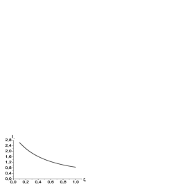
Figure 3: Universal functions $I_{\pm}(\xi)$ which define the total scattering cross-section as the functions of the parameter $\xi$ for the cases of repulsion and attraction.

Now let us consider another integral characteristic of the scattering process, namely, the transport cross-section which is very important value for a lot of applications. It is defined by the formula

$$\sigma_{tr}=\int_{0}^{\pi}2\xi\sinh(\pi\xi)|G_{1}(\pm i\xi,iz)|^{2}r^{2}\sin\theta(1-\cos\theta)d\theta.$$ (28)

If one uses the variable z in this integral and comes back to the hypergeometric function of the 2-nd genus, Eq.(28) transforms as follows

$$\sigma_{tr}=\frac{2\pi\xi^{2}}{k^{2}}e^{\mp\pi\xi}I^{tr}_{\pm}(\xi);$$

$$I^{tr}_{\pm}(\xi)=\int_{0}^{2kr}|U(1\pm i\xi,1,iz)|^{2}zdz.$$ (29)

The integrand function for the transport cross-section is essentially suppressed in the range of small angles in comparison with the total cross-section. Therefore $\sigma_{tr}$ is defined by only the logarithm of the distance to the observation point unlike to $\sigma_{tot}$ proportional to this distance. Besides, this function decreases rather slowly for the large $z$ and we can’t use the trick analogous to Eq. (III) for $\sigma_{tr}$. Nevertheless a series of transformations of the integral $I^{tr}_{\pm}(\xi)$ permits one to find the analytical dependence on the coordinate $r$ with an accuracy of the order $(kr)^{-1}$. Let us separate the integral on two parts by the following way

$$I^{tr}_{\pm}(\xi)=\int_{0}^{1}|U(1\pm i\xi,1,iz)|^{2}zdz+\int_{1}^{2kr}|U(1\mp i\xi,1,iz)|^{2}zdz.$$

If one uses the asymptotic formulas for the hypergeometric functions mors

$$|U(1\pm i\xi,1,iz)|^{2}\simeq\frac{e^{\pm\pi\xi}}{z^{2}}+O[(kr)^{-3}],$$

the second term in this integrals is transformed identically

$$\int_{1}^{2kr}[|U(1\pm i\xi,1,iz)|^{2}-\frac{e^{\pm\pi\xi}}{z^{2}}]zdz+\int_{1}^{2kr}\frac{e^{\pm\pi\xi}}{z}dz.$$

The second integral here is calculated analytically but now the integrand expression in the first one decreases rather quickly and the estimation analogous to (III) can be used

$$\int_{1}^{\infty}[|U(1\pm i\xi,1,iz)|^{2}-\frac{e^{\pm\pi\xi}}{z^{2}}]zdz-\int_{2kr}^{\infty}[|U(1\pm i\xi,1,iz)|^{2}-\frac{e^{\pm\pi\xi}}{z^{2}}]zdz\simeq$$

$$\int_{1}^{\infty}[|U(1\pm i\xi,1,iz)|^{2}-\frac{e^{\pm\pi\xi}}{z^{2}}]zdz+O[(kr)^{-1}].$$ (30)

In the result the transport cross-section is defined by well converged integrals

$$\sigma_{tr}=\frac{2\pi\xi^{2}e^{\mp\pi\xi}}{k^{2}}\{\int_{0}^{1}|U(1\pm i\xi,1,iz)|^{2}zdz+$$

$$\int_{1}^{\infty}[|U(1\pm i\xi,1,iz)|^{2}-\frac{e^{\pm\pi\xi}}{z^{2}}]zdz+e^{\pm\pi\xi}\ln(2kr)\}.$$ (31)

Fig.4 shows the results of numerical calculation of the universal functions $I^{tr}_{\pm}(\xi)=[k^{2}\sigma_{tr}-2\pi\xi^{2}\ln(2kr)]$.

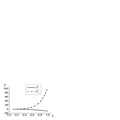
Figure 4: Universal functions $I^{tr}_{\pm}(\xi)$ for the transport cross-section in the cases of attraction and repulsion. Solid line - the case of attraction, dashed line - the case of repulsion

IV Scattering operator and conservation of the flux in scope of the stationary theory

As it follows from the results of the preceding section the integral scattering characteristics calculated on the basis of nonasymptotic consideration increase together with distance $r$ to the observation point. It seems for the first sight that it can contradict to the conservation of the total flux of the particles when $r$ becomes rather large. However, let us show that this dependence expresses only the fact that the potential influences on the scattering process at any distance from the center but the scattering flux remains essentially less than integral incidence flux at any $r$. For qualitative analysis one should take into account that in scope of the stationary scattering theory the quantum state of the incident particle is described by the plane wave. Then the total incidence flux $J_{0}$ through the sphere with radius $r$ corresponding to the observation point can be estimated as follows

$$J_{0}\simeq j_{0}\pi r^{2}.$$

Then the ratio of the scattering and incident integral fluxes is

$$\frac{j^{tot}_{sc}}{j_{0}}\simeq\frac{\sigma_{tot}}{r^{2}}=\frac{2\pi}{kr}\xi^{2}I_{\pm}\ll 1.$$ (32)

It is also important to consider this problem more precisely. It is known landau1 that the condition of the total flux conservation leads to the ”optical” theorem in the quantum theory of scattering by short-range potential when the amplitude of scattering to the zero angle is the finite value. We use the same approach landau1 in order to find the consequence of this condition in the case of nonasymptotic analysis of the Coulomb scattering.

Let us represent general solution of the Schrödinger equation in the case of the elastic scattering as the linear combination of the functions (II) with arbitrary coefficients $\Phi(\vec{n})$ which define the amplitudes of probability to find the state with the wave vector $\vec{k}=k\vec{n}$ in the initial packet:

$$\Psi(\vec{r})=\int\Phi(\vec{n})\psi_{\vec{k}}(\vec{r})d\Omega_{\vec{n}}=N\int\Phi(\vec{n})e^{ikr\vec{n}\vec{n}^{\prime}}F[\pm i\xi,1,ikr(1-\vec{n}\vec{n}^{\prime})]d\Omega_{\vec{n}}=$$

$$\int\Phi(\vec{n})[(z)^{\pm i\xi}\frac{e^{ikr}}{\Gamma(\pm i\xi)}G_{1}(\pm i\xi,iz)+(z)^{\mp i\xi}\frac{e^{ikr\vec{n}\vec{n}^{\prime}}}{\Gamma(\pm i\xi)}G_{2}(\pm i\xi,iz)]d\Omega_{\vec{n}};$$

$$\vec{n}^{\prime}=\frac{\vec{r}}{r};\quad z=kr(1-\vec{n}\vec{n}^{\prime}),$$ (33)

$d\Omega_{\vec{n}}$ is the element of the solid angle in the direction of the vector $\vec{n}$.

In accordance with the physical interpretation of the contributions defined by the functions $G_{1},G_{2}$ to the total wave function (II), the first term in Eq.(IV) describes that part of the integral scattering operator landau1 which corresponds to the formation of the scattering wave. The term, proportional to the function $G_{2}$, describes the deformation of the wave packet conditioned by change of the plane wave in the Coulomb field. One can estimate the second term by the same method that was used for proof of the ”optical” theorem in the case of short-range potential landau1 . If the condition $kr\gg 1$ is fulfilled, the main contributions to this integral are defined by the small intervals near the points of the stationary phases when integrating over $\vec{n}$ . These points correspond to the vectors $\vec{n}_{1}=-\vec{n}^{\prime}$ and $\vec{n}_{2}=\vec{n}^{\prime}$. Near the first point the variable $z\simeq 2kr$ is very large. Therefore one can use the asymptotic expression for the function $G_{2}(\pm i\xi,iz)$ and the integrand has no singularities in this case. In the result the contribution to the integral from the domain close to this point defines the converged spherical wave with the standard logarithmic distortion of its phase landau1

$$\sim 2\pi i\frac{e^{-ikr\mp i\xi\ln 2kr}}{kr}\Phi(-\vec{n}^{\prime}).$$

When estimating the contribution to the integral from the second point of stationary phase corresponding to scattering at small angles one should take into account that the function $G_{2}(\pm i\xi,iz)$ has the logarithmic singularity in the point $z=0$. Nevertheless, the rather smooth weight function $\Phi(\vec{n})$ can be removed from the integral in the point $\vec{n}=\vec{n}^{\prime}$. It leads to the following estimation:

$$\sim 2\pi\Phi(\vec{n})e^{\mp\frac{\pi}{2}\xi}\frac{e^{ikr}}{kr\Gamma(\pm i\xi)}[\int_{0}^{\infty}(z)^{\mp i\xi}e^{-iz}G_{2}(\pm i\xi,iz)dz-\int_{2kr}^{\infty}(z)^{\mp i\xi}e^{-iz}G_{2}(\pm i\xi,iz)dz].$$

The second integral in this expression can be omitted in the limit $kr\gg 1$ and the initial wave function is represented in the form:

$$\Psi(\vec{r})\simeq 2\pi i\frac{e^{-ikr\mp i\xi\ln 2kr}}{kr}\Phi(-\vec{n}^{\prime})-2\pi i\frac{e^{ikr}}{kr}[A\Phi(\vec{n}^{\prime})+\int\hat{f}(\vec{n},\vec{n}^{\prime})\Phi(\vec{n})d\vec{n}];$$

$$A=\frac{ie^{\mp\frac{\pi}{2}\xi}}{\Gamma(\pm i\xi)}\int_{0}^{\infty}(z)^{\mp i\xi}e^{-iz}G_{2}(\pm i\xi,iz)dz;$$

$$\hat{f}(\vec{n},\vec{n}^{\prime})=\frac{ikr}{2\pi\Gamma(\pm i\xi)}e^{\mp\frac{\pi}{2}\xi}e^{\pm i\xi\ln kr}(1-\vec{n}\vec{n}^{\prime})^{\pm i\xi}G_{1}[\pm i\xi,ikr(1-\vec{n}\vec{n}^{\prime})].$$ (34)

It is more convenient to rewrite this expression in terms of the hypergeometric function of the 2-nd genus

$$A=ie^{\mp\frac{\pi}{2}\xi}\int_{0}^{\infty}e^{-iz}U(\pm i\xi,1,iz)dz;$$

$$\hat{f}(\vec{n},\vec{n}^{\prime})=-\frac{ikr\Gamma(1\mp i\xi)}{2\pi\Gamma(\pm i\xi)}e^{\mp\frac{\pi}{2}\xi}U[1\mp i\xi,1,-ikr(1-\vec{n}\vec{n}^{\prime})].$$ (35)

Now the function is represented as the superposition of the ingoing and outgoing spherical waves and it permits one to introduce the scattering matrix Landau1 as the following integral operator:

$$\hat{S}(\vec{n},\vec{n}^{\prime})\simeq A\delta_{\vec{n},\vec{n}^{\prime}}+\hat{f}(\vec{n},\vec{n}^{\prime}).$$ (36)

Here $\delta_{\vec{n},\vec{n}^{\prime}}$ is the unit operator which corresponds to the wave passed without scattering and the parameter A defines the change of its amplitude (in the case of the short-range potential $A=1$ landau1 ). The integral over angles from the operator $\int\hat{f}^{*}(\vec{n},\vec{n}^{\prime})\hat{f}(\vec{n}^{\prime},\vec{n})d\vec{n}^{\prime}$ coincides exactly with the expression for the total cross section (III). Long-range character of the potential is appeared in the fact that the scattering matrix elements depend on the coordinate $r$. However, it is very important to introduce such operator because just it defines the kernel of the collision integral in the kinetic equations for description of various transport processes kinetic . But if one uses such operator in the collision integral for one-particle distribution function the additional averaging over the coordinate should be fulfilled. Dependence of the function $f(\vec{n}^{\prime},\vec{n})$ on the coordinate is rather smooth , therefore the value $r$ in this function can be substituted as an average distance between the scattering centers if the correlation between these centers can be neglected (see below $\S 6$). Analogous substitution was used in some well-known models for regularization of the transport cross section of scattering by the charged impurities in semiconductors herring , conwell .

Unitary property of the matrix $\hat{S}(\vec{n},\vec{n}^{\prime})$ leads to the ”optical” theorem in the case of short-range potentials landau1 . But if one uses this condition in the case of Coulomb potential there is the problem that the operator $\hat{f}(\vec{n},\vec{n}^{\prime})$ has the logarithmic singularity in the limit of coinciding arguments and one should define the way for calculating integral from the product of singular functions $\hat{f}(\vec{n},\vec{n}^{\prime})$ and $\delta_{\vec{n},\vec{n}^{\prime}}$ in the operator $\hat{S}\hat{S}^{+}$ . Actually it means that the asymptotic estimation of the integral in Eq.(IV) is unavailable for the operator which is quadratic over the scattering matrix. Therefore let us analyze separately the conservation of flux considering the following integral

$$I=\int d\vec{S}(\vec{\nabla}j(\vec{r}))\equiv\int((\vec{r}j(\vec{r}))rd\Omega_{\vec{n}};$$

$$\vec{j}(\vec{r})=\frac{\hbar}{2mi}\{\Psi^{*}(\vec{r})\vec{\nabla}\Psi(\vec{r})-\Psi(\vec{r})\vec{\nabla}\Psi^{*}(\vec{r})\},$$ (37)

with the total wave function (IV).

When the superposition (IV) is used in formula (IV) one can take into account the completeness of the coefficients $\Phi(\vec{n})$. Then integration over all directions in this integral is equivalent to the integral from the flux $\vec{j}_{st}$ calculated by means of the general formula (IV) but with the stationary wave functions $\psi_{\vec{k}}(\vec{r})$ defined by Eq. (II) ( let us consider the attractive potential for definiteness )

$$\vec{j}_{st}(\vec{r})=\frac{\hbar\pi\xi e^{\pi\xi}}{m\sinh\pi\xi}\{\vec{k}|F[i\xi,1,i(kr-\vec{k}\vec{r})]|^{2}-\xi(\vec{k}-k\frac{\vec{r}}{r})\Im(FF_{1}^{*})\};$$

$$\vec{\nabla}F[i\xi,1,i(kr-\vec{k}\vec{r})]=\xi(\vec{k}-k\frac{\vec{r}}{r})F[i\xi+1,2,i(kr-\vec{k}\vec{r})]\equiv\xi(\vec{k}-k\frac{\vec{r}}{r})F_{1}.$$ (38)

Certainly, the value $I$ is equal to zero identically because of the flux conservation for the stationary scattering problem. The ”optical” theorem is followed from this condition if the asymptotic form (5) for the wave function can be used landau1 . But in the considered problem this condition means that the flux directed along the vector $\vec{k}$ (it defines change of the intensity of the incident wave), and the scattering flux along the vector $\vec{r}$ are connected as follows

$$\int d\Omega_{\vec{n}}(\vec{k}\vec{n})|F[i\xi,1,i(kr-\vec{k}\vec{r})]|^{2}=\xi\int d\Omega_{\vec{n}}(\vec{k}\vec{r}-k)\Im(FF_{1}^{*}).$$ (39)

As it was shown above the integrals over the angle for the Coulomb scattering problem include essential contribution defined by ”near” zone. Therefore the both parts of Eq.(39) depend on the coordinate $r$ and the standard asymptotic expressions for ”optical” theorem is inapplicable because the total cross section and the scattering amplitude at zero angle are tending to infinity in this case. But if one shows that the leading terms of Eq.(39) are equal in the limit of large r ($kr\gg 1$) it can be considered as the analog of the ”optical” theorem for the Coulomb potential.

In order to prove it let us use new variable for the integrals in Eq. (39)

$$z=kr-\vec{k}\vec{r};\quad\sin\theta d\theta=\frac{dz}{kr},$$

and transform them as follows

$$\int_{0}^{2kr}|F(i\xi,1,iz)|^{2}dz=\int_{0}^{2kr}\frac{z}{kr}\{|F|^{2}+\xi\Im[F(-i\xi,1,-iz)F(i\xi+1,2,iz)]\}dz.$$ (40)

One can estimate the integrals from the confluent hypergeometric functions in the range $kr\gg 1$ by means of the following approach. Integral in the left side of Eq.(40) can be transformed identically

$$J_{1}=\int_{0}^{2kr}|F(i\xi,1,iz)|^{2}dz=\lim_{\delta\rightarrow 0}[\int_{0}^{\infty}|F|^{2}e^{-\delta z}dz-\int_{2kr}^{\infty}|F|^{2}e^{-\delta z}dz].$$ (41)

The parameter $\delta\rightarrow 0$ is introduced for the regularization of both integrals at upper limit. The asymptotic form of the function F can be used in the second term and the first term can be expressed through the hypergeometric function $F(\alpha,\beta,\gamma,z)$ by means of the formula (see, for example landau1 )

$$J(\lambda)=\int_{0}^{\infty}e^{-\lambda z}z^{\gamma-1}F(\alpha,\gamma,kz)F(\alpha^{\prime},\gamma,k^{\prime}z)dz=$$

$$\Gamma(\gamma)\lambda^{\alpha+\alpha^{\prime}-\gamma}(\lambda-k)^{-\alpha}(\lambda-k^{\prime})^{-\alpha^{\prime}}F[\alpha,\alpha^{\prime},\gamma,\frac{kk^{\prime}}{(\lambda-k)(\lambda-k^{\prime})}].$$ (42)

When the integrals from the functions with different second arguments are calculated, the following recursion relation can be used mors

$$F(\alpha+1,\gamma+1,z)=\frac{\gamma}{z}[F(\alpha+1,\gamma,z)-F(\alpha,\gamma,z)].$$

Let us write also the leading terms of the asymptotic expansions for the functions F $F_{1}$ which are used for the integrals in the limits $(2kr,\infty)$

$$F(i\xi,1,iz)\simeq e^{-\pi\xi/2}[\frac{z^{-i\xi}}{\Gamma(1-i\xi)}(1-\frac{i\xi^{2}}{z}+\frac{\xi^{2}(1+i\xi)^{2}}{2z^{2}})-\frac{iz^{i\xi}e^{iz}}{z\Gamma(i\xi)}];$$

$$F_{1}=F(i\xi+1,2,iz)\simeq\frac{ie^{-\pi\xi/2}}{z}[\frac{z^{-i\xi}}{\Gamma(1-i\xi)}(1-\frac{\xi(1+i\xi)}{z})-\frac{z^{i\xi}e^{iz}}{\Gamma(1+i\xi)}(1-\frac{\xi(1-i\xi)}{z})];$$

In the result the leading term in the left side of Eq. (40) is the following

$$J_{1}\simeq e^{-\pi\xi}\frac{\sinh\pi\xi}{\pi\xi}\{2kr-$$

$$\frac{1}{kr}[\xi^{2}+\Re\{\frac{\Gamma(1+i\xi)e^{-2ikr-2i\xi\ln 2kr}}{\Gamma(-i\xi)}\}]\}+O[\frac{1}{(kr)^{2}}].$$ (43)

This value defines variation of the flux directed along the incident wave vector and it grows linearly together with the distance from the scattering center analogously to the total cross section. As it was mentioned above (Eq. (IV)), this growth is not connected with increase of the particle flux but describes distorted part of the wave front which is extended together with $r$ because of long-range character of the potential.

Calculation of the integral

$$J_{2}=\frac{1}{kr}\int_{0}^{2kr}|F(i\xi,1,iz)|^{2}zdz$$

by means of the analogous technique leads to the following result

$$J_{2}\simeq e^{-\pi\xi}\frac{\sinh\pi\xi}{\pi\xi}\{2kr+\frac{2}{kr}[\xi^{2}(-\frac{1}{2}-\Re\psi(1+i\xi)+\ln 2kr)-$$

$$\Re\{\frac{\Gamma(1+i\xi)e^{-2ikr-2i\xi\ln 2kr}}{\Gamma(-i\xi)}\}]\}+O[\frac{1}{(kr)^{2}}],$$ (44)

where $\psi(x)$ is the logarithmic derivative of $\Gamma$ - function mors .

The last integral in Eq. (40)

$$J_{3}=\frac{\xi}{kr}\int_{0}^{2kr}z\Im[F(-i\xi,1,-iz)F(i\xi+1,2,iz)]dz=$$

$$-\frac{\xi}{kr}\int_{0}^{2kr}\Re[F(-i\xi,1,-iz)F(i\xi+1,1,iz)]dz,$$ (45)

transforms as follows

$$J_{3}\simeq-\frac{2}{kr}e^{-\pi\xi}\frac{\sinh\pi\xi}{\pi\xi}\{\xi^{2}(-\Re\psi(1+i\xi)+\ln 2kr)-$$

$$\frac{1}{2}\Re[\frac{\Gamma(1+i\xi)e^{-2ikr-2i\xi\ln 2kr}}{\Gamma(-i\xi)}]\}+O[\frac{1}{(kr)^{2}}].$$ (46)

Substitution of Eqs. (IV) - (IV) to Eq. (40) shows that it is satisfied with the considered accuracy. Besides, one can see that the left side of Eq. (40) coincides with the total cross section (III) in the limit $kr\gg 1$, and the right side of Eq. (40) transforms to the imaginary part of the scattering operator (40) with $\vec{n}=\vec{n}^{\prime}$. So, we can consider this calculation as the proof of the ”optical” theorem for the Coulomb scattering problem.

V Movement of the wave packet in the Coulomb field

As it follows from the results of the preceding sections, regularization of the Rutherford cross section is defined by the characteristic angle

$$\theta_{0}=\sqrt{\frac{2}{kr}},$$ (47)

which corresponds to the boundary of ”near” zone and is considered as the kinematic parameter (KP) of the system. However, in real scattering experiments the incident particle is actually represented by the localized wave packet goldberger . Besides, the Coulomb potential is screened at some distance $R_{s}$, depending on the properties of the medium where the collision is happened. Therefore in general case the problem is characterized by some additional parameters that can be considered as the external parameters (EP). So, it is essential to estimate the conditions when the KP is more important for the cross section regularization that the EP. We will take into account two the most essential EP: the screening angle $\theta_{s}$ the incident angle parameter $\theta_{int}$, depending on the wave packet transversal width a and defining the zone of interference between the incident and scattered waves (see also Sec.2). The simple estimation of these parameters leads to

$$\theta_{s}=\frac{1}{kR_{s}},\qquad\theta_{int}=\frac{a}{r}.$$ (48)

Evidently, the kinematic regularization is the most essential if the angle width of the near zone is larger in comparison with the characteristic angle intervals connected with EP, that is the following conditions are fulfilled

$$\theta_{0}>\theta_{s},\quad\frac{kR^{2}_{s}}{r}>1;\qquad\theta_{0}>\theta_{int},\quad\frac{ka^{2}}{r}<1.$$ (49)

The first inequality depends on the mechanism of screening and should be analyzed for every concrete system as it will be considered below (Sec.6) for the scattering by impurities in semiconductors. In order to take into account the finite size of the wave packet in the second inequality in (49) one should use the time-dependent theory of collisions goldberger , 1971 , that we will consider in this section.

Let us suppose that the initial state of the particle in the moment $t=0$ is defined by the wave packet in the following form

$$\Psi_{\vec{k}}(\vec{r},0)=\int d\vec{q}\Phi(\vec{q}-\vec{k})e^{i\vec{q}(\vec{r}-\vec{r}_{0})}\equiv e^{i\vec{k}(\vec{r}-\vec{r}_{0})}G(|\vec{r}-\vec{r}_{0}|),$$

$$G(\rho)=\int d\vec{p}\Phi(\vec{p})e^{i\vec{p}\vec{\rho}},$$ (50)

where $\vec{r}_{0}$ is the coordinate corresponding to the initial position of the wave packet ; $\Phi(\vec{p})$ are the amplitudes of probabilities of the wave vector distribution near the center $\vec{k}$ in the initial state; $G(\rho)$ is the function which describes the form of the localized wave packet in the coordinate space goldberger .

In order to describe evolution of the wave packet (V) it should be expanded in the solutions of the stationary Schrödinger equation with the Coulomb potential 1971 (let us consider the attractive potential for the definiteness )

$$\psi_{\vec{k}}(\vec{r})=Ne^{i\vec{k}\vec{r}}F[i\xi_{k},1,i(kr-\vec{k}\vec{r})].$$

In the standard experimental setting (Fig.5) the initial position of the wave packet corresponds to the condition $z_{0}\rightarrow-\infty$. In this case the stationary wave function $\psi_{\vec{k}}(\vec{r})$ coincides with the plane wave goldberger and the expansion of $\Psi_{\vec{k}}(\vec{r},0)$ in the functions $\psi_{\vec{k}}(\vec{r})$ includes the same coefficients as in the formula (V) with an accuracy to the terms of the order $|z_{0}|^{-1}$ conditioned by the logarithmic distortion of the wave front in the Coulomb field landau1 . In the result the wave function describing the wave packet state in an arbitrary moment of time has the following form

$$\Psi_{\vec{k}}(\vec{r},t)=\int d\vec{q}\Phi(\vec{q}-\vec{k})e^{i\vec{q}\vec{r}}e^{-i\vec{q}\vec{r}_{0}}e^{\pi\xi_{q}/2}\Gamma(1-i\xi_{q})F[i\xi_{q},1,i(qr-\vec{q}\vec{r})]e^{-i\hbar q^{2}t/2m}.$$ (51)

As it was investigated in detail in the monography goldberger the wave packet spread (diffraction) can be neglected during time of the interaction in real scattering experiments. This corresponds to the following approximations in the integrand expression in the formula (51)

$$\vec{q}-\vec{k}=\vec{p};\quad p\ll k;\quad\frac{\hbar q^{2}}{2m}\simeq\frac{\hbar k^{2}}{2m}+(\vec{p}\vec{v});\quad\xi_{q}\simeq\xi=\frac{\alpha}{\hbar v};\quad q\simeq k+\frac{(\vec{p}\vec{k})}{k},$$ (52)

where $\vec{v}=\hbar\vec{k}/m$ is the group velocity of the center of the wave packet coinciding with the velocity of classical particles.

Let us remind briefly results of the time-dependent collision theory in the case of the short-range potential when the asymptotic form (5) of the stationary wave function can be used for analysis of the wave packet evolution goldberger

$$\Psi_{\vec{k}}(\vec{r},t)=\int d\vec{q}\Phi(\vec{q}-\vec{k})e^{-i\vec{q}\vec{r}_{0}}[e^{i\vec{q}\vec{r}}+f(\theta_{q})\frac{e^{iqr}}{r}]e^{-i\hbar q^{2}t/2m},$$ (53)

where $\theta_{q}$ is the angle between the vectors $\vec{q}$ and $q\vec{r}/r$.

Now one can use the expansions (52) and to find the following result for the function $\Psi_{\vec{k}}(\vec{r},t)$

$$\Psi_{\vec{k}}(\vec{r},t)\simeq\{e^{i\vec{k}\vec{r}}G(|\vec{r}-\vec{r}_{0}-\vec{v}t|)+f(\theta_{k})\frac{e^{ikr}}{r}G(|r\frac{\vec{k}}{k}-\vec{r}_{0}-\vec{v}t|)\}e^{-i\vec{k}\vec{r}_{0}}e^{-i\hbar k^{2}t/2m}.$$ (54)

Fig.5 shows the sketch of distribution of the probability density corresponding to the wave packet (54) in some moment t. It demonstrates two essential results which represents actually the basis for use the quantum mechanical stationary scattering theory for description of the collisions between real particles goldberger . Firstly, the overlapping of the fluxes corresponding to the incident ( first term in the formula (54)) and scattering particles is essential only in the above-mentioned interference zone with the angular width $\theta_{int}=a/r$ and they can be considered separately out of this domain. Besides, the scattering flux is localized in the spherical layer with the average radius $r\simeq|\vec{r}_{0}+\vec{v}t|$ and width $\sim a$. The angular distribution of the scattering particle in the limits of this layer is completely defined by the scattering amplitude $f(\theta_{k})$ calculated on the basis of the stationary theory.

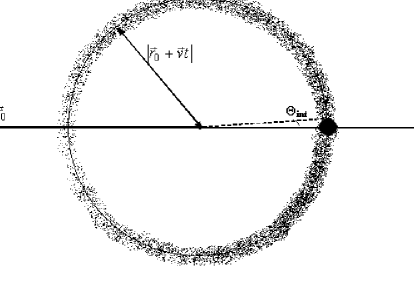
Figure 5: Sketch of distribution of the probability density corresponding to the wave packet (54) in some moment t

The expansions (52) can be used in the integral (53) in the case of the integrand without singularities in the range of the variable variation . This condition doesn’t satisfied for the asymptotic form (5) in the case of the Coulomb field because the Rutherford amplitude includes unintegrable singularity. Let us show, however, that the representation of the wave packet analogous to the formula (54) is justified also for the Coulomb problem if the expansion (54) is built on the basis nonasymptotic representation (II) for the confluent hypergeometric function:

$$\Psi_{\vec{k}}(\vec{r},t)=\int d\vec{q}\Phi(\vec{q}-\vec{k})e^{-i\vec{q}\vec{r}_{0}}[(z_{q})^{i\xi_{q}}\frac{e^{iqr}}{\Gamma(i\xi_{q})}G_{1}(i\xi_{q},iz_{q})+$$

$$(z_{q})^{-i\xi_{q}}\frac{e^{i\vec{q}\vec{r}}}{\Gamma(i\xi_{q})}G_{2}(i\xi_{q},iz_{q})]e^{-i\hbar q^{2}t/2m};$$

$$z_{q}=qr-\vec{q}\vec{r}.$$ (55)

The functions $G_{1,2}$ are rather smooth and integrable. One can use the expansion (52) for their arguments if the following condition is satisfied in the region $z_{q}\leq 1$ of the most essential variation of these functions

$$z_{k}\geq\vec{p}(r\frac{\vec{k}}{k}-\vec{r})\simeq pr\theta_{p}.$$ (56)

If the spread of the wave packet is neglected, the value $|\vec{p}|$ can be estimated as $|\vec{p}|\simeq k\theta_{p}\simeq ka/r$ ( is the characteristic linear size of the wave packet localization in space) and the condition (56) leads to the inequality

$$\theta^{2}\simeq\frac{1}{kr}\geq(\frac{a}{r})^{2},\quad\frac{ka^{2}}{r}\leq 1.$$ (57)

It coincides with the above mentioned estimation (49) considered on the basis of the qualitative analysis.

In the result the functions $G_{1,2}$ in the formula (V) can be removed out of the integral with the arguments corresponding to the center of the wave packet and it leads to the expression

$$\Psi_{\vec{k}}(\vec{r},t)=[(z_{k})^{i\xi_{k}}\frac{e^{ikr}}{\Gamma(i\xi_{k})}G_{1}(i\xi_{k},iz_{k})G(|r\frac{\vec{k}}{k}-\vec{r}_{0}-\vec{v}t|)+$$

$$(z_{k})^{-i\xi_{k}}\frac{e^{i\vec{k}\vec{r}}}{\Gamma(i\xi_{k})}G_{2}(i\xi_{k},iz_{k})G(|\vec{r}-\vec{r}_{0}-\vec{v}t|)]e^{-i\vec{k}\vec{r}_{0}}e^{-i\hbar k^{2}t/2m};$$

$$z_{k}=kr-\vec{k}\vec{r}.$$ (58)

It means that the scattering process in the Coulomb field can be considered on the basis of the stationary theory as it takes place in the case of the short-range potential. Besides, the incident and scattered wave packets are extending in the space separately excluding unessential domain of their overlapping.

VI Calculation of the charge carrier mobility in the extrinsic semiconductors

It is important to consider the concrete physical system where the described peculiarities of the scattering process in the Coulomb field can be appeared for some observed characteristics. Accordingly to the estimation (49), it is possible if the following inequality is fulfilled

$$\frac{kR^{2}_{s}}{r}>1.$$ (59)

Here $R_{s}$ is the screening radius of the Coulomb potential in a medium and it depends on the screening mechanism in the system. The value r is defined by the distance between the scattering center and detector or by the average distance between two subsequent collisions if the scattering operator (III) is used for the description of kinetic processes in the system.

In the present paper the nonasymptotic scattering theory will be used for analysis of the charge carrier mobility in the extrinsic semiconductors for low temperature. In this case concentration of the impurity centers defines both the type of the carriers and their concentration and also the main contribution to the resistance of the semiconductor ziman . The problem was recently analyzed in detail in the paper poklonskii and results of the various phenomenological models for regularization of the Rutherford cross-section were compared with the experimental data poklonskii . It was shown that the wide used models of Brooks-Herring herring , and Conwell-Weisskopf conwell don’t describe completely the experimental dependence of the mobility on the temperature and impurity concentration. The authors of the paper poklonskii fitted the experimental data essentially better by means of an additional phenomenological parameter with the physical meaning of the characteristic time of the collision. It seems to us that such parameter takes into account partly the influence of the ”near” zone (see Sec.2) on the formation of the scattered flux. So, the regularization of the scattering problem in the Coulomb field is of interest not only as the methodical problem but also as the applied one.

Let us consider the extrinsic semiconductor with the concentrations of the donors $n_{1}$ and acceptors $n_{2}$ in the charge states $Z_{1}e$ and $Z_{2}e$ correspondingly (in the most of real structures the impurities with the charge $|Z_{1,2}|=1$ are mainly important ), e is the absolute value of the electron charge.

In general case the value $n_{e}$ is defined by both the thermally excited carriers and the carriers conditioned by the impurities. The semiconductors with the wide forbidden zone were analyzed in the paper poklonskii and the value $n_{e}$ can be estimated as

$$n_{e}\simeq Z_{1}n_{1}-Z_{2}n_{2}=n,$$

for the considered low temperature.

Let us introduce also another parameter which is more spread in the semiconductor physics: K is the compensation and is usually a quite small value $K\simeq 0.1$ poklonskii

$$n_{1}=\frac{n}{Z_{1}-KZ_{2}},\quad n_{2}=\frac{nK}{Z_{1}-KZ_{2}},\quad K=\frac{n_{2}}{n_{1}}.$$ (60)

It is well known ziman that the Coulomb potential screening in semiconductors is defined by several factors. From one side, there is the static dielectric constant $\epsilon$ conditioned by the electrons from the valency zone which doesn’t change the long-range character of the potential. From the other side, the Debye screening of the potential by free electrons (or holes) leads to its cut off on the distance ziman

$$R_{s}\simeq\sqrt{\frac{\epsilon k_{B}T}{4\pi e^{2}n_{e}}},$$ (61)

where $k_{B}$ is the Boltzmann constant; $T$ is the crystal temperature; $n_{e}$ is the concentration of free charge carriers (electrons in the conductivity zone for n-type semiconductors or holes in the valency zone for p-type semiconductors).

The average distance r between scattering centers and the characteristic wave vector for the carriers in the formula (59) can be estimated as

$$r\simeq n^{-1/3};\qquad k=\frac{\sqrt{2m^{*}E}}{\hbar}\simeq\frac{\sqrt{3m^{*}k_{B}T}}{\hbar},$$

with $m^{*}$ as the carrier effective mass.

In the result the condition (59) leads to the following inequality

$$\frac{(3\epsilon m^{*})^{1/2}(k_{B}T)^{3/2}}{4\pi e^{2}\hbar n^{2/3}}>1,$$ (62)

which is fulfilled in the entire range of the density and temperature considered in poklonskii .

In the most applications the theoretical estimation of the carrier mobility is based on the approximation of relaxation time $\tau$ and the Maxwell velocity distribution. It leads to the following formula (n-type semiconductors are considered for the definiteness) ziman

$$\mu=\frac{e}{m^{*}}<\tau>$$ (63)

$$<\tau>=[\int_{0}^{\infty}E^{3/2}e^{-E/k_{B}T}]^{-1}\int_{0}^{\infty}\tau(E)E^{3/2}e^{-E/k_{B}T}.$$ (64)

Here the relaxation time is supposed to be averaged on the energy of carriers with the Maxwell distribution.

It is known blekmor that if the several mechanisms of scattering take place (in our case there are scattering by donors and acceptors), the more accurate result the additional averaging on the types of scattering centers should be fulfilled:

$$\ \tau(E)=\frac{\tau_{1}(E)\tau_{2}(E)}{\tau_{1}(E)+\tau_{2}(E)},$$

$$\tau_{1,2}(E)=\frac{1}{n_{1,2}v\sigma_{tr1,2}},$$ (65)

where the indexes 1,2 correspond to the scattering by donors and acceptors; $\sigma_{tr1,2}$ is the transport cross-section for the cases of the attraction and repulsion. In accordance with Sec.3 these values are defined by the formulas :

$$\sigma_{tr1,2}=\frac{2\pi\xi_{1,2}^{2}e^{\mp\pi\xi_{1,2}}}{k^{2}}\int_{0}^{2kr_{1,2}}|U(1\pm i\xi_{1,2},1,iz)|^{2}zdz.$$ (66)

We use here the more accurate formula than Eq.(III) because in this case the condition $kr\gg 1$ can not be fulfilled.

The parameters of interaction between carriers and scattering centers in the considered cases are the following

$$\xi_{1,2}(E)=\frac{Z_{1,2}e^{2}}{\epsilon\hbar v}$$

and the static dielectric constant of the crystal is taken into account.

Accordingly to the formulae (66) the transport cross section depends on the potential charge as distinct of its calculation with the Rutherford cross section. The similar effect (”phase shift”) is well known for extrinsic semiconductors and considers usually by means of the Fridel sum rule fridel . Indefinite parameter $r$ is included in Eq.(66). If the value $\mu$ is calculated by the totally microscopic way it should be averaged on the space distribution of the impurities in the sample. It is equivalent to the integration of the expression (63) by $r$ taking into account Eq.(66). However, the transport cross-section has the smooth logarithmic behavior on $r$ which can substituted in Eq.(66) as the average distance between the impurities with the considered accuracy. Then the value $r=0.5n^{-1/3}_{i}$ can be used in Eq.(66) analogously to the both models herring , and conwell .

It is convenient to define the auxiliary value $\sigma_{tr}^{\prime}$ so, that

$$\sigma_{tr}=2\pi\frac{\xi^{2}}{k^{2}}\sigma_{tr}^{\prime}.$$

Then nonasymptotic calculation leads to

$$\sigma_{tr1,2}^{\prime}=e^{\mp\pi\xi_{1,2}}\int_{0}^{2kr_{1,2}}|U(1\pm i\xi_{1,2},1,iz)|^{2}zdz,$$ (67)

with the values

$$r_{1}=\frac{(Z_{1}-KZ_{2})^{1/3}}{2n^{1/3}},\quad r_{2}=\frac{(Z_{1}-KZ_{2})^{1/3}}{2(nK)^{1/3}},$$

which are defined by the half of the average distance between the donors and acceptors correspondingly.

In the result the following expression for the carrier mobility can be obtained:

$$\mu=\frac{2^{5/2}\epsilon^{2}(k_{B}T)^{3/2}}{3\pi^{3/2}e^{3}m^{\ast 1/2}n}\int_{0}^{\infty}\frac{x^{3}e^{-x}}{Z_{1}^{2}\sigma_{tr1}^{\prime}(x)+KZ_{2}^{2}\sigma_{tr2}^{\prime}(x)}dx.$$ (68)

The integrals over energies can be estimated by the standard way conwell : the smoothly changing functions can be taken out of the integrals with argument $x=3$ when the energy distribution function has the maximum value. It leads to the following analytical expression for the mobility:

$$\mu=\frac{2^{7/2}\epsilon^{2}(Z_{1}-KZ_{2})(k_{B}T)^{3/2}}{\pi^{3/2}e^{3}m^{\ast 1/2}n(Z_{1}^{2}\sigma_{tr1}^{\prime}(3k_{B}T)+KZ_{2}^{2}\sigma_{tr2}^{\prime}(3k_{B}T))}.$$ (69)

In the case $Z_{1}=Z_{2}=1$ it transforms as follows

$$\mu=\frac{2^{7/2}\epsilon^{2}(1-K)(k_{B}T)^{3/2}}{\pi^{3/2}e^{3}m^{\ast 1/2}n(\sigma_{tr1}^{\prime}(3k_{B}T)+K\sigma_{tr2}^{\prime}(3k_{B}T))}.$$ (70)

We can compare it with the analogous formula in the framework of the Conwell-Weisskopf model conwell

$$\mu_{CW}=\frac{2^{7/2}\epsilon^{2}(1-K)(k_{B}T)^{3/2}}{\pi^{3/2}e^{3}m^{\ast 1/2}n(1+K)\ln(1+(\frac{3\epsilon k_{B}T(1-K)^{1/3}}{Ze^{2}(n(1+K))^{1/3}})^{2})}.$$ (71)

The results of calculation by means of Eqs.(70) and their comparison with the Conwell-Weisskopf model results are shown in Fig.6. The same figure shows that the dependence of the mobility on the temperature and compensation K in our consideration differ essentially on the results of the Conwell-Weisskopf model conwell based on the Rutherford cross section with the phenomenological regularization. In principle, such distinction can be discovered in some experiments.

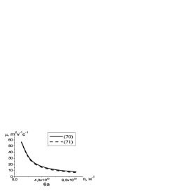
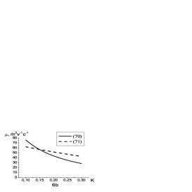
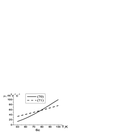
Figure 6: Comparison of the mobilities calculated with the nonasymptotic transport cross-section (solid line) and in the framework of the Conwell-Weisskopf model (dashed line)(6a - dependence on the impurity concentration; 6b - on the compensation; 6c - on the temperature). The following parameters were used $T=78,\epsilon=10,m=0.2m_{0},K=0.15$.

VII Acknowledgments

Authors are grateful to Prof. N.A.Poklonskii for useful discussions and International Scientific Technical Center (Grant B-626) for the support of this work .

References

- (1) L.D.Landau and E.M.Lifshitz, Quantum Mechanics: Non-Relativistic Theory, 3rd edition Vol 3, (Pergamon Press, London, 1997).
- (2) R.G.Newton, Theory of Waves and Particles, 2nd edition , (McGraw Hill, New York, 1982).
- (3) L.D.Landau and E.M.Lifshitz, Mechanics, (Nauka, Moscow, 1965)
- (4) D.Sing, Classical Dynamics,( Fizmatgiz, Moscow, 1963).
- (5) H.Brooks, Phys. Rev., 83,(1951), 879.
- (6) E.Conwell and V.F.Wesskopf, Phys. Rev., 77,(1950), 388.
- (7) N.A.Poklonskii, S.A.Vyrko et al.,Applied Phys., 93,(2003), 9749.
- (8) B.K.Ridley, Quantum Processes in Semicoducters, (Clarendon Press, Oxford, 1999); K.Seeger, Semiconductor Physics, (Springer-Verlag, Berlin, 1999).
- (9) S.W.Kim, H-K.Park, H-S. Sim and H.Shomerus,J.Phys.A: Math. and Gen., 36,(2003), 1299.
- (10) K.Elmer,J. Phys.D: Applied Phys., 34,(2001), 3097.
- (11) K. Harigawa,J.Phys: Condensed Matter, 12,(2000), 7069. 388.
- (12) V.G.Baryshevskii, L.N.Korennaya and I.D.Feranchuk,Soviet Physics JETP, 34,(1972), 249.
- (13) M.Goldberger and K.Watson, Collision Theory,(Wiley, New York, 1964).
- (14) W.Zackowicz,J.Phys.A: Math. Gen., 36,(2003), 4445.
- (15) J.Jackson , Classical electrodynamics, (John Willey and sons, New-York - London, 1962).
- (16) Ph.Mors and H.Feshbach Methods of Theoretical Physics, (Mc-Graw-Hill Book Co., New York, 1953).
- (17) J.M.Ziman Principles of The Theory of Solids, (At The University Press, Cambridge, 1972).
- (18) A.D.Boardman, D.W.Henry Phys. stat., sol. (b),60,(1973), 633.
- (19) J. Blekmor Solid state physics, (Nauka, Moscow, 1988).
- (20) E.M.Lifshitz, L.P. Pitaevski Physical kinetics , Moscow,1979.
- (21) A.F. Nikiforov, V.B.Uvarov Special functions of mathematical physics, (Nauka, Moscow, 1984).