Active and Passive Quantum Erasers for Neutral Kaons

Abstract

Quantum marking and quantum erasure are discussed for the neutral kaon system. Contrary to other two–level systems, strangeness and lifetime of a neutral kaon state can be alternatively measured via an “active” or a “passive” procedure. This offers new quantum erasure possibilities. In particular, the operation of a quantum eraser in the “delayed choice” mode is clearly illustrated.

I Introduction

The introduction of quantum marking and erasure by Scully and Drühl [1, 2] in 1982 opened the possibility to discuss some of the most relevant and subtle aspects of quantum measurement. Indeed, since the foundation of quantum mechanics, one is well aware of the crucial role played by measurement devices; a role which, occasionally, is even extended to conscious observers, as in the well known proposal by Wigner. Quantum marking and erasure are useful tools to investigate these basic issues. Up to now, experimental tests of quantum erasure have been performed with atom interferometers [3] and entangled photon pairs produced via spontaneous parametric down–conversion (SPDC) [4, 5, 6, 7, 8, 9]. The general purpose of the present paper is to extend these quantum eraser considerations to entangled massive particles, i.e., $K^{0}\bar{K}^{0}$ pairs produced in $\phi$–resonance decays [10] or proton–antiproton annihilations at rest [11].

The basic idea behind quantum marking and erasure is that two indistinguishable —and thus potentially interfering— amplitudes of a quantum system, the object, can be made distinguishable thanks to the entanglement between the object and a second quantum system, the meter, which thus carries a kind of quantum mark. In ordinary two–path interferometric devices, the latter, marked system is frequently called a “which way” detector. If the information stored in the “which way” detector is even in principle accessible, the object system looses all its previous interference abilities. However, if one somehow manages to “erase” the meter mark and thus the distinguishability of the object amplitudes, the original object interference effects can be restored. This is achieved by correlating the outcomes of the measurements on the object system with those of suitable erasing measurements on the meter system.

The case in which the meter is a system distinct and spatially separated from the object is of particular interest. Indeed, in this case the decision to erase or not the meter mark and the distinguishability of the object amplitudes —and therefore to observe or not interference— can be taken long after the measurement on the object system has been completed. Quantum erasure is then performed in the so called delayed choice mode which best captures the essence and most subtle aspects of this phenomenon [1, 2, 12, 13]. This mode of quantum erasure can be applied to entangled $K^{0}\bar{K}^{0}$ pairs as well as to SPDC photon pairs, but, specific of the kaon case is the possibility that the erasure operation can be carried out via two distinct procedures: either actively, i.e., by exerting the free will of the experimenter, or passively, i.e., randomly exploiting a particular quantum–mechanical property of the meter system. This opens new possibilities for quantum erasure with kaons.

The first specific purpose of this paper is to discuss the existence of these two different active and passive quantum erasure procedures for neutral kaons. A second, twofold purpose is to show both the simplicity of the delayed choice mode of quantum erasure and its extension to passive measurements when operated with neutral kaons. These kaons turn out to be most suitable for achieving these two purposes.

II Measurements on neutral kaons

Contrary to what happens with other two–level quantum systems such as spin–$1/2$ particles or photons, neutral kaons only exhibit two different measurement bases [14, 15]: the strangeness and the lifetime bases.

The strangeness basis, $\{K^{0},\bar{K}^{0}\}$ with $\langle K^{0}|\bar{K}^{0}\rangle=0$, is the appropriate one to discuss strong production and reactions of kaons. If a dense piece of nucleonic matter is inserted along a neutral kaon beam, the incoming state is projected either into a $K^{0}$ by the strangeness conserving strong interaction $K^{0}p\rightarrow K^{+}n$ or into a $\bar{K}^{0}$ via $\bar{K}^{0}p\rightarrow\Lambda\pi^{+}$, $\bar{K}^{0}n\rightarrow\Lambda\pi^{0}$ or $\bar{K}^{0}n\rightarrow K^{-}p$. These strangeness detections are totally analogous to the projective von Neumann measurements of two–channel analyzers for polarized photons or Stern–Gerlach setups for spin–$1/2$ particles. By inserting the piece of matter along a kaon beam, one induces an active measurement of strangeness.

The strangeness content of neutral kaon states can be alternatively determined by observing their semileptonic decay modes. Indeed, these semileptonic decays obey the well tested $\Delta S=\Delta Q$ rule which allows the modes

$$K^{0}(\bar{s}d)\to\pi^{-}(\bar{u}d)\;+\;l^{+}\;+\;\nu_{l}\;,\;\;\bar{K}^{0}(s\bar{d})\to\pi^{+}(u\bar{d})\;+\;l^{-}\;+\;\bar{\nu}_{l},$$ (1)

where $l$ stands for $e$ or $\mu$, but forbids decays into the respective charge conjugated modes. Obviously, the experimenter cannot induce a kaon to decay semileptonically and not even at a given time: he or she can only sort at the end of the day all observed events in proper decay modes and time intervals. We call this discrimination between $K^{0}$ and $\bar{K}^{0}$ via the identification of the kaon semileptonic decay modes a passive measurement of strangeness.

The detection efficiency for both active and passive strangeness measurements is rather limited. In the former case, the detection efficiency is close to $1$ only for ultrarelativistic kaons; indeed, by Lorentz contraction the piece of matter is seen by the incoming kaon as extremely dense and kaon–nucleon strong interactions become much more likely than kaon weak decays. In the case of passive strangeness detection, the efficiency is given by the $K_{L}$ and $K_{S}$ semileptonic branching ratios, which are $\simeq 0.66$ and $\simeq 1.1\times 10^{-3}$, respectively. These limited detection efficiencies, which originate a serious problem [14, 16] when discussing Bell–type tests for entangled kaons [15, 17, 18, 19, 20], do not introduce any conceptual difficulty here. They simply represent a practical difficulty in obtaining large statistical samples.

The second basis, the lifetime basis $\{K_{S},K_{L}\}$, consists of the short– and long–lived states having well defined masses $m_{S(L)}$ and decay widths $\Gamma_{(S)L}$. It is the appropriate basis to discuss free space propagation, with:

$$|K_{S}(\tau)\rangle=e^{-i\lambda_{S}\tau}|K_{S}\rangle,\;\;|K_{L}(\tau)\rangle=e^{-i\lambda_{L}\tau}|K_{L}\rangle,$$ (2)

and $\lambda_{S(L)}=m_{S(L)}-i\Gamma_{S(L)}/2$. These states preserve their own identity in time, but, since $\Gamma_{S}\simeq 579\,\Gamma_{L}$ [21], the $K_{S}$ component of a neutral kaon extincts much faster than the $K_{L}$ component. To observe if a kaon is propagating as a $K_{S}$ or $K_{L}$ at (proper) time $\tau$, one has to identify at which time it subsequently decays. Kaons which show a prompt decay, i.e., a decay between $\tau$ and $\tau+\Delta\tau$, have to be identified as $K_{S}$’s, while those decaying later than $\tau+\Delta\tau$ have to be identified as $K_{L}$’s. The probabilities for wrong $K_{S}$ or $K_{L}$ identification are then given by $\exp(-\Gamma_{S}\,\Delta\tau)$ and $1-\exp(-\Gamma_{L}\,\Delta\tau)$, respectively. With $\Delta\tau=4.8\,\tau_{S}$, both $K_{S}$ and $K_{L}$ misidentification probabilities are equal and reduce to $\simeq 0.8$% [14, 18, 22]. Such a procedure, in which the experimenter chooses to allow for free space propagation, represents an active measurement of lifetime.

Since four decades one knows that the neutral kaon system violates $CP$ symmetry. Among other things, this implies that the weak interaction eigenstates are not strictly orthogonal to each other, $\langle K_{S}|K_{L}\rangle=2({\rm Re}\,\varepsilon)/(1+|\varepsilon|^{2})\simeq 3.2\cdot 10^{-3}$ [21, 23]. However, by neglecting these small $CP$ violation effects one can discriminate between $K_{S}$’s and $K_{L}$’s by leaving the kaons to propagate in free space and observing their distinctive nonleptonic $K_{S}\to 2\pi$ or $K_{L}\to 3\pi$ decay modes. This represents a passive measurement of lifetime, since the type of kaon decay modes —nonleptonic in the present case, instead of semileptonic as before— cannot be in any way influenced by the experimenter. The measurement procedure is determined by the quantum dynamics of kaon decays.

Summarizing, we have two conceptually different experimental procedures —active and passive— to measure each one of the only two neutral kaon observables: strangeness or lifetime. The active measurement of strangeness is monitored by strangeness conservation while the corresponding passive measurement is assured by the $\Delta S=\Delta Q$ rule. Active and passive lifetime measurements are efficient thanks to the smallness of $\Gamma_{L}/\Gamma_{S}$ and $\varepsilon$, respectively. The existence of these two procedures is of no interest when testing Bell inequalities with kaons, where active measurements must be considered [14, 15]. However, it opens new possibilities for kaonic quantum erasure experiments which have no analog for any other two–level quantum system considered up to date.

III Single kaons: time evolution and measurements

Let us start discussing the time evolution of a single neutral kaon which is initially produced (say) as a $K^{0}$. Just after production, at $\tau=0$, it is described by the equal superposition of the two lifetime eigenstates, $|K^{0}(0)\rangle=\{|K_{S}\rangle+|K_{L}\rangle\}/\sqrt{2}$, and, according to Eq. (2), it starts propagating in free space in the coherent superposition:

$$|K^{0}(\tau)\rangle=\frac{1}{\sqrt{2}}\{e^{-i\lambda_{S}\tau}|K_{S}\rangle+e^{-i\lambda_{L}\tau}|K_{L}\rangle\}\;.$$ (3)

Note that the state $|K^{0}(\tau)\rangle$ evolves through a single spatial trajectory comprising automatically —i.e., with no need of any kind of double–slit apparatus— the two differently propagating components $K_{S}$ and $K_{L}$. This generates the well known strangeness or $K^{0}$–$\bar{K}^{0}$ oscillations. Note also that, since $\Gamma_{S}\simeq 579\,\Gamma_{L}$, these two components are intrinsically marked by their remarkably distinct decay widths. At $\tau=0$ this lifetime mark is inoperative and there is no information on which component is actually propagating; $K_{S}$–$K_{L}$ interference and thus $K^{0}$–$\bar{K}^{0}$ oscillations are maximal around $\tau=0$. However, for kaons surviving after some time $\tau$, $K_{S}$ propagation is known to be less likely than $K_{L}$ and partial “which width” information is obtained; interference and oscillation phenomena are thus diminished. This happens in the same way as when one obtains “which way” information in two–path interferometric devices, as recently discussed in Ref. [24] in terms of quantitative complementarity. This dedicated analysis shows that a variety of double–slit experiments with photons or neutrons, as well as Mott scattering experiments with identical nuclei, admit the very same description as the present oscillations of the neutral kaon system. But two advantages of the latter system are obvious: it does not need any kind of double–slit device nor any marking procedure; indeed, both features are inherently supplied by Nature.

Active and passive measurements of strangeness or lifetime on single kaon states evolving, for instance, as in Eq. (3) offer no difficulties and have been performed since long time ago.

For the two possible active measurements one either inserts or not a dense piece of matter at a (time–of–flight) distance $\tau$ along the kaon trajectory. The corresponding quantum–mechanical probabilities are simply derived by projecting Eq. (3) either into the strangeness or into the lifetime basis. By properly normalizing Eq. (3) to undecayed kaons, the following oscillating probabilities for $K^{0}$ and $\bar{K}^{0}$ detection at time $\tau$ are obtained:

$$P\left[K^{0}(\tau)\right]={1\over 2}\left[1+{\cal V}_{0}(\tau)\cos(\Delta m\,\tau)\right],$$ (4)

$$P\left[\bar{K}^{0}(\tau)\right]={1\over 2}\left[1-{\cal V}_{0}(\tau)\cos(\Delta m\,\tau)\right].$$ (5)

In these expressions:

$${\cal V}_{0}(\tau)=\frac{1}{\cosh(\Delta\Gamma\tau/2)}$$ (6)

is the time–dependent visibility of the strangeness oscillations, $\Delta m\equiv m_{L}-m_{S}$ and $\Delta\Gamma\equiv\Gamma_{L}-\Gamma_{S}$. Instead, no oscillations are predicted for lifetime measurements:

$$P\left[K_{L}(\tau)\right]={1\over 1+e^{+\Delta\Gamma\tau}}\;,$$ (7)

$$P\left[K_{S}(\tau)\right]={1\over 1+e^{-\Delta\Gamma\tau}}\;.$$ (8)

Passive measurements of strangeness or lifetime on single kaon states are slightly less direct. One has to measure the $\tau$–dependent decay rate $\Gamma(f,\tau)$ which is defined as the number of decays into the mode $f$ occurring between $\tau$ and $\tau+d\tau$ divided by $d\tau$ and by the total number of initial $K^{0}$’s. Its formal expression is given by:

$$\Gamma(f,\tau)\equiv\int d\Omega_{f}\,p(f,\tau),$$ (9)

where the integration is over the phase space of the decay product state $f$ ($f=\pi\pi$, $\pi\pi\pi$, $\pi^{-}l^{+}\nu_{l}$ or $\pi^{+}l^{-}\bar{\nu}_{l}$) and:

$$p(f,\tau)\equiv\frac{1}{2}\biggl{|}e^{-i\lambda_{S}\,\tau}\langle f|T|K_{S}\rangle+e^{-i\lambda_{L}\,\tau}\langle f|T|K_{L}\rangle\biggl{|}^{2}.$$ (10)

The decay rate $\Gamma(f,\tau)$ is normalized such that $\sum_{f}\int d\tau\,\Gamma(f,\tau)=1$ and allows one to determine the single kaon detection probabilities through the relation:

$$P\left[K_{f}(\tau)\right]=\frac{\Gamma(f,\tau)}{\Gamma(K_{f}\to f)\,N(\tau)},$$ (11)

which reproduces the predictions (4)–(8) of active measurements. In Eq. (11), $K_{f}=K_{S}$, $K_{L}$, $K^{0}$ or $\bar{K}^{0}$ and $N(\tau)\equiv[e^{-\Gamma_{L}\,\tau}+e^{-\Gamma_{L}\,\tau}]/2$ is a normalization factor taking into account the extinction with time of the beam. Moreover, the decay widths $\Gamma(K_{f}\to f)$, where $K_{f}\to f$ stands for the four identifying decay modes, $K_{S}\to\pi\pi$, $K_{L}\to\pi\pi\pi$, $K^{0}\to\pi^{-}l^{+}\nu_{l}$ and $\bar{K}^{0}\to\pi^{+}l^{-}\bar{\nu}_{l}$, are given by:

$$\Gamma(K_{f}\to f)\equiv\int d\Omega_{f}|\langle f|T|K_{f}\rangle|^{2}=\frac{BR(K_{L}\to f)\,\Gamma_{L}}{|\langle K_{f}|K_{L}\rangle|^{2}}=\frac{BR(K_{S}\to f)\,\Gamma_{S}}{|\langle K_{f}|K_{S}\rangle|^{2}},$$ (12)

where the second (third) equality is only defined for nonvanishing values of $\langle K_{f}|K_{L}\rangle$ ($\langle K_{f}|K_{S}\rangle$) and $BR(K_{L(S)}\to f)$ is the branching ratio for the decay $K_{L(S)}\to f$.

The experimental equivalence of both measurement procedures and the agreement with quantum–mechanical predictions have already been proved [21, 25, 26].

IV Entangled kaon pairs: time evolution and measurements

Let us now consider two–kaon entangled states which are analogous to the standard and widely used two–photon entangled states produced by SPDC. From both $\phi$–meson resonance decays [10] or $S$–wave proton–antiproton annihilation [11], one starts at time $\tau=0$ with the state:

$$|\phi(0)\rangle=\frac{1}{\sqrt{2}}\left[|K^{0}\rangle_{l}|\bar{K}^{0}\rangle_{r}-|\bar{K}^{0}\rangle_{l}|K^{0}\rangle_{r}\right]=\frac{1}{\sqrt{2}}\left[|K_{L}\rangle_{l}|K_{S}\rangle_{r}-|K_{S}\rangle_{l}|K_{L}\rangle_{r}\right],$$ (13)

where $l$ and $r$ denote the “left” and “right” directions of motion of the two separating kaons and $CP$–violating effects are neglected in the last equality. Note that this state is antisymmetric and maximally entangled in the two observable bases.

After production, the left and right moving kaons evolve according to Eq. (2) up to times $\tau_{l}$ and $\tau_{r}$, respectively, thus leading to the state:

$$|\phi(\tau_{l},\tau_{r})\rangle=\frac{1}{\sqrt{2}}\left\{e^{-i(\lambda_{L}\tau_{l}+\lambda_{S}\tau_{r})}|K_{L}\rangle_{l}|K_{S}\rangle_{r}-e^{-i(\lambda_{S}\tau_{l}+\lambda_{L}\tau_{r})}|K_{S}\rangle_{l}|K_{L}\rangle_{r}\right\}.$$ (14)

By normalizing to kaon pairs with both members surviving up to $(\tau_{l},\tau_{r})$, one obtains the state:

$$|\phi(\Delta\tau)\rangle=\frac{1}{\sqrt{1+e^{\Delta\Gamma\Delta\tau}}}\biggl{\{}|K_{L}\rangle_{l}|K_{S}\rangle_{r}-e^{i\Delta m\Delta\tau}e^{{1\over 2}\Delta\Gamma\Delta\tau}|K_{S}\rangle_{l}|K_{L}\rangle_{r}\biggr{\}},$$ (15)

where $\Delta\tau\equiv\tau_{l}-\tau_{r}$, or, equivalently:

$$|\phi(\Delta\tau)\rangle = \frac{1}{2\sqrt{1+e^{\Delta\Gamma\Delta\tau}}}\left\{(1-e^{i\Delta m\Delta\tau}e^{{1\over 2}\Delta\Gamma\Delta\tau})\left[|K^{0}\rangle_{l}|K^{0}\rangle_{r}-|\bar{K}^{0}\rangle_{l}|\bar{K}^{0}\rangle_{r}\right]\right.$$ (17)

$$\left.+(1+e^{i\Delta m\Delta\tau}e^{{1\over 2}\Delta\Gamma\Delta\tau})\left[|K^{0}\rangle_{l}|\bar{K}^{0}\rangle_{r}-|\bar{K}^{0}\rangle_{l}|K^{0}\rangle_{r}\right]\right\},$$

in the strangeness basis.

Thanks to this normalization, one works with bipartite two–level systems as for photon or spin–$1/2$ entangled pairs. For a detailed description of the time evolution of entangled neutral kaon pairs, see Refs. [17, 20]. The analogy between state (15) and the polarization–entangled two–photon [idler ($i$) plus signal ($s$)] state $|\Psi\rangle=\left[|V\rangle_{i}|H\rangle_{s}-e^{i\Delta\phi}|H\rangle_{i}|V\rangle_{s}\right]/\sqrt{2}$, where $\Delta\phi$ is a relative phase under control by the experimenter, is obvious.

A Active measurements on both kaons

Active joint measurements on two–kaon states are again quite obvious. Active strangeness measurements on both sides require strangeness detectors inserted at $\tau_{l}$ and $\tau_{r}$. This corresponds to act with the projectors $P_{i}^{l}P_{j}^{r}$, where $P_{i(j)}=|K^{0}\rangle\langle K^{0}|$ or $|\bar{K}^{0}\rangle\langle\bar{K}^{0}|$, on the state (17). The probabilities to observe like– and unlike–strangeness joint events are:

$$P\left[K^{0}(\tau_{l}),K^{0}(\tau_{r})\right]=P\left[\bar{K}^{0}(\tau_{l}),\bar{K}^{0}(\tau_{r})\right]=\frac{1}{4}\left[1-{\cal V}(\Delta\tau)\cos(\Delta m\,\Delta\tau)\right],$$ (18)

$$P\left[K^{0}(\tau_{l}),\bar{K}^{0}(\tau_{r})\right]=P\left[\bar{K}^{0}(\tau_{l}),K^{0}(\tau_{r})\right]=\frac{1}{4}\left[1+{\cal V}(\Delta\tau)\cos(\Delta m\,\Delta\tau)\right],$$ (19)

respectively, where:

$${\cal V}(\Delta\tau)=\frac{1}{\cosh(\Delta\Gamma\Delta\tau/2)}.$$ (20)

First, we note that for $\Delta\tau=0$ we have perfect EPR–correlations: since ${\cal V}(0)=1$, the like–strangeness probabilities vanish and the unlike–strangeness probabilities take the maximum value. Second, $\Delta m\,\Delta\tau$ plays the same role as the relative orientation of polarization analyzers for entangled photon pairs. The kaon mass difference $\Delta m$ introduces automatically a time dependent relative phase between the two kaon amplitudes of Eq. (15). However, opposite to the photon case, the visibility of Eq. (20) decreases as $|\Delta\tau|$ increases.

If one wants to measure, actively, strangeness on the left and lifetime on the right, one has to remove the piece of matter on the right to allow for free kaon propagation in space. One then measures the following non–oscillating joint probabilities:

$$P\left[K^{0}(\tau_{l}),K_{S}(\tau_{r})\right]=P\left[\bar{K}^{0}(\tau_{l}),K_{S}(\tau_{r})\right]=\frac{1}{2\left(1+e^{\Delta\Gamma\Delta\tau}\right)},$$ (21)

$$P\left[K^{0}(\tau_{l}),K_{L}(\tau_{r})\right]=P\left[\bar{K}^{0}(\tau_{l}),K_{L}(\tau_{r})\right]=\frac{1}{2\left(1+e^{-\Delta\Gamma\Delta\tau}\right)},$$ (22)

which are directly obtained from state (15) by acting with the projectors $P_{i}^{l}P_{j}^{r}$, where $P_{i(j)}=|K_{S}\rangle\langle K_{S}|$, $|K_{L}\rangle\langle K_{L}|$, $|K^{0}\rangle\langle K^{0}|$ or $|\bar{K}^{0}\rangle\langle\bar{K}^{0}|$.

B Passive measurements on both kaons

Passive joint measurements are somewhat more involved. In this case, one allows the entangled kaon pairs to propagate freely in space and identifies the kaon decay times and modes. As discussed in detail in Ref. [15], one has to measure the ($\tau_{l}$– and $\tau_{r}$–dependent) joint decay rate:

$$\Gamma(f_{l},\tau_{l};f_{r},\tau_{r})\equiv\int d\Omega_{f_{l}}\,d\Omega_{f_{r}}\,p(f_{l},\tau_{l};f_{r},\tau_{r}),$$ (23)

which is the obvious generalization of the previously defined single kaon decay rate $\Gamma(f,\tau)$, with:

$$p(f_{l},\tau_{l};f_{r},\tau_{r}) \equiv \frac{1}{2}\biggl{|}e^{-i(\lambda_{L}\tau_{l}+\lambda_{S}\tau_{r})}\langle f_{l}|T|K_{L}\rangle_{l}\langle f_{r}|T|K_{S}\rangle_{r}$$ (25)

$$-e^{-i(\lambda_{S}\tau_{l}+\lambda_{L}\tau_{r})}\langle f_{l}|T|K_{S}\rangle_{l}\langle f_{r}|T|K_{L}\rangle_{r}\biggl{|}^{2}.$$

The joint decay rate $\Gamma(f_{l},\tau_{l};f_{r},\tau_{r})$ is normalized such that $\sum_{f_{l},f_{r}}\int d\tau_{l}\,d\tau_{r}\,\Gamma(f_{l},\tau_{l};f_{r},\tau_{r})=1$ and supplies the joint detection probabilities through the relation [15]:

$$P\left[K_{f_{l}}(\tau_{l}),K_{f_{r}}(\tau_{r})\right]=\frac{\Gamma(f_{l},\tau_{l};f_{r},\tau_{r})}{\Gamma(K_{f_{l}}\to f_{l})\,\Gamma(K_{f_{r}}\to f_{r})\,N(\tau_{l},\tau_{r})},$$ (26)

where $N(\tau_{l},\tau_{r})\equiv e^{-(\Gamma_{L}+\Gamma_{S})(\tau_{l}+\tau_{r})/2}\cosh\left[\Delta\Gamma(\tau_{l}-\tau_{r})/2\right]$ is a normalization factor depending on both $\tau_{l}$ and $\tau_{r}$ which accounts for the extinction of the beams, while $K_{f_{l}}$, $K_{f_{r}}=K_{S}$, $K_{L}$, $K^{0}$ or $\bar{K}^{0}$.

In the good approximation of $CP$ conservation and the validity of the $\Delta S=\Delta Q$ rule, it is then easy to see that the physical meaning and the quantum–mechanical expressions for the probabilities obtained through Eq. (26) coincide with the results (18)–(22) corresponding to active joint measurements. However, while the latter probabilities are measured either by actively inserting or removing a piece of nucleonic matter in the beams, the measurement method via Eq. (26) is completely different: a quantum–mechanical process alone (namely, the dynamics of kaon decays) decides if each one of the two kaons of a given pair is going to be measured either in the strangeness or in the lifetime basis. The experimenter remains totally passive in such measurements.

C Combining active and passive measurements

One can similarly combine an active measurement on one side with a passive measurements on the other. Let us consider, for instance, an active strangeness measurement on the left with outcome $K^{0}$ and a passive lifetime or strangeness measurement on the right with outcome $K_{f_{r}}=K_{S}$, $K_{L}$, $K^{0}$ or $\bar{K}^{0}$. One then has to determine the relevant joint probabilities via the relation:

$$P\left[K^{0}(\tau_{l}),K_{f_{r}}(\tau_{r})\right]=\frac{\Gamma[K^{0},\tau_{l};f_{r},\tau_{r}]}{\Gamma(K_{f_{r}}\to f_{r})\,N(\tau_{l},\tau_{r})},$$ (27)

where:

$$\Gamma[K^{0},\tau_{l};f_{r},\tau_{r}]\equiv\int d\Omega_{f_{r}}\,p[K^{0},\tau_{l};f_{r},\tau_{r}],$$ (28)

$$p[K^{0},\tau_{l};f_{r},\tau_{r}]\equiv\frac{1}{4}\biggl{|}e^{-i(\lambda_{L}\tau_{l}+\lambda_{S}\tau_{r})}\langle f_{r}|T|K_{S}\rangle_{r}-e^{-i(\lambda_{S}\tau_{l}+\lambda_{L}\tau_{r})}\langle f_{r}|T|K_{L}\rangle_{r}\biggl{|}^{2},$$ (29)

and the normalization factor, $N(\tau_{l},\tau_{r})\equiv e^{-(\Gamma_{L}+\Gamma_{S})(\tau_{l}+\tau_{r})/2}\cosh\left[\Delta\Gamma(\tau_{l}-\tau_{r})/2\right]$, has the same expression of the previous case with passive joint measurements. The normalization of the decay rate $\Gamma[K^{0},\tau_{l};f_{r},\tau_{r}]$ reads $\sum_{f_{r}}\int d\tau_{r}\,\Gamma[K^{0},\tau_{l};f_{r},\tau_{r}]=N(\tau_{l},0)/2$.

As expected, the quantum–mechanical results of Eqs. (18)–(22) are again reproduced.

V Quantum eraser experiments for kaons

Several quantum eraser experiments have already been performed [4, 5, 6, 7, 8, 9]. They used SPDC to produce a two–photon maximally entangled state which is the analog of the kaon state of Eq. (15). One photon of the pair is considered as the object system. On this photon one may obtain “which way” ($WW$) information by a suitable measurement on the other photon, the meter. Different strategies —quite often by exploiting photon polarizations, as in Refs. [4, 7, 8, 9]— are used for marking and subsequently erasing the meter $WW$ information. But all these photon experiments need a kind of double–slit mechanism in order to allow for a “wave–like” behaviour of the object system. Moreover, they also require a meter marking procedure.

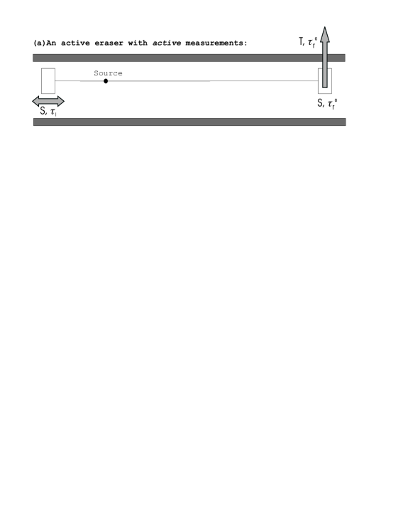
By contrast, the two–kaon entangled state of Eq. (15) is given by Nature evolving through two amplitudes which are automatically marked. One can then play the game of the quantum marking and erasure experiments. Four possible experiments are illustrated in Fig.1 and discussed in the following. In the first three cases, (a),(b) and (c), the left moving kaon is the object system; on this kaon one performs active strangeness measurements at different $\tau_{l}$–values to scan for possible strangeness oscillations. The right moving kaon is the meter system; it carries “which width” ($W\mathcal{W}$) information which can be actively (passively) erased by a suitable active (passive) measurement at a fixed time $\tau_{r}^{0}$ (at times below $\tau_{r}^{0}$). In the fourth experiment, (d), passive measurements are performed on both sides. In this case, it is not clear which kaon plays the role of the meter.

(a) Active eraser with active measurements

In a first setup, strangeness detectors are actively inserted along each beam. Only kaon pairs which survive up to both detectors are considered in this case. We clearly observe $K_{S}$–$K_{L}$ interference in the coincident counts of the object–meter system with a visibility ${\cal V}(\tau_{l}-\tau_{r}^{0})$ given by Eq. (20). More precisely, one expects fringes for unlike–strangeness joint detections [Eq. (19)] and anti–fringes for like–strangeness joint detections [Eq. (18)]. In a second setup, the strangeness detector previously placed along the right beam is removed and only right going kaons that survive up to $\tau_{r}^{0}$ are considered. One then observes the lifetime of the meter and thus obtains $W\mathcal{W}$ information for the object kaon as well. The object–meter coincidence counts do not exhibit interference: they follow the non–oscillatory behaviour of Eqs. (21) and (22) with $\Delta\tau=\tau_{l}-\tau_{r}^{0}$.

Hence, we have an experiment consisting of two setups in which the experimenter can erase or not the $W\mathcal{W}$ information by placing or not, at will, the strangeness detector along the right beam. The first setup reveals the “wave–like” behaviour of the object kaon: if $\tau_{l}=\tau_{r}^{0}$, the two propagating components $K_{S}$ and $K_{L}$ of the object are completely indistinguishable because their marks are made totally inoperative by the strangeness measurement on the meter kaon. One gets interferences with maximal visibility as in conventional double–slit experiments with indistinguishable paths. However, for entangled neutral kaons the visibility ${\cal V}(\tau_{l}-\tau_{r}^{0})$ of Eq. (20) decreases with $|\tau_{l}-\tau_{r}^{0}|$ and vanishes when $|\tau_{l}-\tau_{r}^{0}|\to\infty$; correspondingly, almost full $W\mathcal{W}$ information is obtained for both kaons if $|\tau_{l}-\tau_{r}^{0}|\to\infty$. For a discussion on a quantitative formulation of quantum erasure and the complementarity principle for neutral kaons, see Refs. [22, 26]. The second setup clearly demonstrates the “particle–like” behaviour of the object kaon: no interference is observed because the meter mark is operative and one could gain full $W\mathcal{W}$ information on the right moving kaon. This situation mimics double–slit setups with complete $WW$ information.

This kaon experiment is analogous to the photon experiments of Refs. [4, 6, 7], as discussed in detail in Ref. [22]. Note, however, that in the kaon case the amplitudes are automatically marked and no double–slit device is needed.

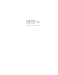
(b) Partially active eraser with active measurements

In this case, a strangeness detector is always placed along the right beam at a fixed time $\tau_{r}^{0}$. However, the experiment also detects and considers eventual decays of the right propagating kaon occurring between the origin and $\tau_{r}^{0}$. In this way, it is the right moving kaon —the meter— that eventually makes the “choice” to show $W\mathcal{W}$ information by decaying before $\tau_{r}^{0}$. If the meter kaon does indeed decay in free space, one measures its lifetime actively, i.e., via a decay time analysis, and obtains $W\mathcal{W}$ information. If no decay is seen, the incoming kaon is projected into one of the two strangeness states at time $\tau_{r}^{0}$ by an active strangeness measurement.

With this single experimental setup one observes the object “wave–like” behaviour (i.e., interference) for some events and the “particle–like” behaviour (i.e., $W\mathcal{W}$ information) for others. The choice to obtain or not $W\mathcal{W}$ information is naturally given by the instability of the meter kaon. However, the experimenter can still choose when —the time $\tau_{r}^{0}$— he or she wants to detect the strangeness of the surviving meter kaons, i.e., to erase the object kaon $W\mathcal{W}$ information. Therefore, there is no control over the marking and erasure operations for individual kaon pairs, but probabilistic predictions for an ensemble of kaon pairs are accessible.

This experiment is analogous to the eraser experiment with entangled photons of Ref. [5]. The role played by the different beam–splitter transmittivities in the photonic experiment is played by the different $\tau_{r}^{0}$’s in the kaon case. If one chooses, for instance, $\tau_{r}^{0}\simeq 4.8\;\tau_{S}$, one half of the events correspond to right $K_{S}$ decays showing no oscillation and the other half will show oscillations and antioscillations in joint strangeness detections.

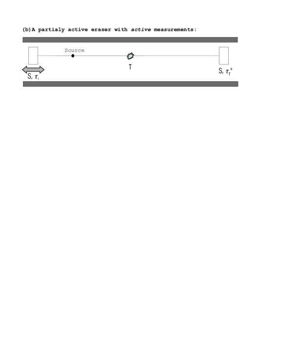
(c) Passive eraser with passive measurement on the meter

In this experiment one looks for the different decay modes in order to identify the right moving meter kaon. This corresponds to a passive measurement of either strangeness or lifetime on the meter. Now one clearly has a completely passive erasing operation on the meter, and the experimenter has no control on the operativeness of the lifetime mark. Only the object system is under some kind of active control —one still makes an active strangeness measurement on the object and considers only kaons surviving up to this detector. Once the decay times of the right kaons are taken into account, one recovers the same joint probabilities as in the previous cases (a) and (b).

This experiment has no analog in any other considered two–level quantum system.

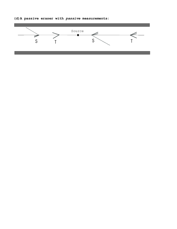
(d) Passive eraser with passive measurements

In this experiment, both kaons evolve freely in space and the experimenter observes, passively, their decay modes. The present procedure constitutes the extreme case of a passive quantum eraser. The experimenter has no control over individual pairs neither on which of the two complementary observables are measured nor when they are measured. The experiment is totally symmetric and thus it shows the full behaviour of the maximally entangled state (15). However, since nothing is actively measured nor erased, strictly speaking one cannot define this experiment as a standard quantum eraser.

Remarkably, the quantum–mechanical predictions for the observable probabilities are again in agreement with those of all the previous experiments. In particular, the joint probabilities for like– and unlike–strangeness passive measurements coincide with those in Eqs. (18) and (19). They are measured by counting and properly sorting the two types of semileptonic decays ($\Delta S=\Delta Q=\pm 1$) at different values of $\tau_{l}$ and $\tau_{r}$.

Also this experiment has no analog in any other considered two–level quantum system.

VI Active and passive delayed choice

An essential and intriguing feature of the quantum eraser is that it can be operated in the so called “delayed choice” mode [1, 2]. If the meter is a system distinct and spatially separated from the object, the decision to erase or not the distinguishing mark on the meter can be taken even after the potentially interfering object system has been detected. The fact that everything works as in the “normal” time ordered mode —in an apparently flagrant violation of causality— has been a source of some controversy [12, 13].

Two specific features of our kaonic case help in this discussion: (i) the two–kaon state is left–right (or, equivalently, object–meter) symmetric, and (ii) time is not only the characteristic parameter distinguishing the two operation modes but also the variable in terms of which strangeness oscillations are observed. The concurrence of these two circumstances in quantum erasure for kaons allows for the following clarifying discussion.

As previously described in the experiment (a) of the previous Section, on the right moving kaon one has the choice to perform, actively, either a strangeness or a lifetime measurement; this is the meter system since it is measured at a fixed time $\tau_{r}^{0}$. For the left moving kaon one measures strangeness at a variable time $\tau_{l}$; this is then the object system. If $\tau_{r}^{0}\leq\tau_{l}$, one operates in the normal, non–controversial mode: the left and right moving kaons are the object and the meter systems, respectively, and the meter mark is erased prior to the object strangeness measurement, $\tau^{0}_{r\,(\rm meter)}\leq\tau_{l\,(\rm object)}$.

Let us consider now the “delayed choice” case in which at a given $\tau_{l}$, such that $\tau_{l}<\tau_{r}^{0}$, strangeness is measured actively on the left moving kaon. Assume as our first case that one chooses to measure strangeness on the right at $\tau_{r}^{0}$: at these given times $\tau_{l}$ and $\tau_{r}^{0}$ one can momentaneously invert the roles of the object and meter kaons. One then operates as in the normal mode, $\tau_{l\,(\rm meter)}<\tau^{0}_{r\,(\rm object)}$, and thus reobtains the usual oscillations of Eqs. (18)–(20) where both $\cos(\Delta m\,\Delta\tau)$ and $\cosh(\Delta\Gamma\Delta\tau/2)$ are even functions of $\Delta\tau$. Since $\Delta\tau=\tau_{l}-\tau_{r}^{0}$ is a time difference, one can then allow for variations in $\tau_{l}$ and thus reconsider the left moving kaon as the object, oscillating system. Assume in a second case that one chooses to measure actively lifetime instead of strangeness on the right at $\tau_{r}^{0}$: each one of the four possible joint probabilities show the non–oscillating feature. In both cases, the “normal” and “delayed choice” operation modes predict the same results.

It should be drawn to the reader’s attention that the above discussion applies to both active and passive measurements on both the left and right moving kaons. The case in which a passive strangeness measurement is performed on the meter provides a new concept of “delayed choice” that we can call a “passive delayed choice”.

More formally, for active joint measurements we can discuss again the issue in terms of projectors and time evolution operators. The various joint probabilities can be computed as the squared norms of the state

$$P^{l}P^{r}\underbrace{U_{l}(\tau_{l},0)U_{r}(\tau_{r}^{0},0)|\phi(0)\rangle}_{|\phi(\tau_{l},\tau_{r}^{0})\rangle}\;,$$ (30)

where $P^{l,r}$ are the four projectors corresponding to the possible outcomes of each (left or right) measurement and $U_{l,r}$ are the time evolution operators, which are unitary since we retain and normalize to surviving kaon pairs. It is easy to show [17, 20] that the state

$$P^{l}U_{l}(\tau_{l},\tau_{r}^{0})P^{r}\underbrace{U_{l}(\tau_{r}^{0},0)U_{r}(\tau_{r}^{0},0)|\phi(0)\rangle}_{|\phi(\tau_{r}^{0},\tau_{r}^{0})\rangle}$$ (31)

—with operators acting successively in the same order as in the normal mode ($\tau_{r\,(\rm meter)}^{0}\leq\tau_{l\,(\rm object)}$)— has the same squared norm as the previous state (30). This is so thanks to (i) the commutativity of the operators acting on different Hilbert spaces and (ii) the properties of unitary time evolution. In the case of the “delayed choice” mode, the corresponding state —with the appropriate ordering of the operators— is

$$P^{r}U_{r}(\tau_{r}^{0},\tau_{l})P^{l}\underbrace{U_{l}(\tau_{l},0)U_{r}(\tau_{l},0)|\phi(0)\rangle}_{|\phi(\tau_{l},\tau_{l})\rangle}\;,$$ (32)

and has again the same squared norm as the previous two states.

VII Conclusions

Under the assumption of $CP$ conservation and the validity of the $\Delta S=\Delta Q$ rule, we have shown that kaons admit two alternative procedures to measure their two complementary observables, strangeness and lifetime. We call these procedures active and passive measurements. The first one can be seen as an analog to the usual von Neumann projection, while the second one is clearly different and takes advantage of the information spontaneously provided by neutral kaons through their decay modes.

In this paper we propose four different experiments combining active and passive measurement procedures in order to demonstrate the quantum erasure principle for neutral kaons. All the considered experiments lead to the same observable probabilities and —more important for delayed choice considerations— this is true regardless of the temporal ordering of the measurements. In our view, this illustrates the very nature of a quantum eraser experiment: it essentially sorts different events, namely, strangeness–strangeness events representing the “wave–like” property of the object kaon or strangeness–lifetime events representing the “particle–like” property of the object. Time ordering considerations about the measurements are not relevant. The same is true for the measurement methods: active measurements —with the intervention of the experimenter— and passive measurements —with no such intervention— lead to equivalent results.

Neutral kaon experiments verifying the proposed quantum marking and eraser procedures has not been performed up to date. As the only exception, the CPLEAR collaboration [11] did part of the job required in our first setup of experiment (a), showing the entanglement of kaon pairs from $p\bar{p}$ annihilation at rest through a measurement which tested the oscillatory behaviour of strangeness–strangeness joint detections for two values of $\tau_{l}-\tau_{r}$. We think that the experiments proposed in this paper are of interest because they offer a new test of the complementarity principle and shed new light on the very concept of the quantum eraser.

REFERENCES

- [1] M. O. Scully and K. Drhl, Phys. Rev. A 25, 2208 (1982).
- [2] M. O. Scully, B.-G. Englert and H. Walther, Nature 351, 111 (1991).
- [3] S. Drr and G. Rempe, Opt. Commun. 179, 323 (2000).
- [4] T. J. Herzog, P. G. Kwiat, H. Weinfurter and A. Zeilinger, Phys. Rev. Lett. 75, 3034 (1995).
- [5] Y.-H. Kim, R. Yu, S. P. Kulik, Y. Shih and M. O. Scully, Phys. Rev. Lett. 84, 1 (2000).
- [6] T. Tsegaye, G. Bjrk, M. Atatre, A. V. Sergienko, B. E. A. Saleh, and M. C. Teich, Phys. Rev. A 62, 032106 (2000).
- [7] S. P. Walborn, M. O. Terra Cunha, S. Pádua and C. H. Monken, Phys. Rev. A 65, 033818 (2002).
- [8] A. Trifonov, G. Bjrk, J. Sderholm and T. Tsegaye, Eur. Phys. J. D 18, 251 (2002).
- [9] H. Kim, J. Ko, and T. Kim, Phys. Rev. A 67, 054102 (2003).
- [10] For a survey on the physics at a –factory see The Second Dane Physics Handbook, edited by L. Maiani, G. Pancheri and N. Paver (INFN, Laboratori Nazionali di Frascati, 1995).
- [11] A. Apostolakis et al., Phys. Lett. B 422, 339 (1998).
- [12] U. Mohrhoff, Am. J. Phys. 64, 1468 (1996); 67, 330 (1999).
- [13] M. O. Scully, B.-G. Englert and H. Walther, Am. J. Phys. 67, 325 (1999).
- [14] A. Bramon and G. Garbarino, Phys. Rev. Lett. 88, 040403 (2002); 89, 160401 (2002); A. Bramon and M. Nowakowski, Phys. Rev. Lett. 83, 1 (1999).
- [15] B. Ancochea, A. Bramon and M. Nowakowski, Phys. Rev. D 60, 094008 (1999).
- [16] M. Genovese, Phys. Rev. A 69, 022103 (2004).
- [17] G. C. Ghirardi, R. Grassi and T. Weber, Proceedings of the Workshop on Physics and Detectors for Dane, edited by G. Pancheri (INFN, Laboratori Nazionali di Frascati, 1991) p.261.
- [18] P. H. Eberhard, Nucl. Phys. B 398, 155 (1993).
- [19] A. Di Domenico, Nucl. Phys. B 450, 293 (1995); F. Uchiyama, Phys. Lett. A 231, 295 (1997); F. Benatti and R. Floreanini, Phys. Rev. D 57, R1332 (1998); R. Foadi and F. Selleri, Phys. Rev. A 61, 012106 (2000); N. Gisin and A. Go, Am. J. Phys. 69, 264 (2001); R. Dalitz and G. Garbarino, Nucl. Phys. B 606, 483 (2001); M. Genovese, C. Novero and E. Predazzi, Phys. Lett. B 513, 401 (2001). R. A. Bertlmann, W. Grimus and B. C. Hiesmayr, Phys. Lett. A 289, 21 (2001).
- [20] R. A. Bertlmann and B. C. Hiesmayr, Phys. Rev. A 63, 062112 (2001); B. C. Hiesmayr, Ph.D. thesis, University of Vienna, 2002.
- [21] Particle Data Group, K. Hagiwara et al., Phys. Rev. D 66, 010001 (2002).
- [22] A. Bramon, G. Garbarino and B. C. Hiesmayr, Phys. Rev. Lett. 92, 020405 (2004).
- [23] P. K. Kabir, The CP Puzzle (Academic Press, London, 1968).
- [24] A. Bramon, G. Garbarino and B. C. Hiesmayr, Phys. Rev. A 69, 022112 (2004).
- [25] A. Angelopoulos et al., Phys. Rept. 374, 165 (2003); Phys. Lett. 503, 49 (2001): 444, 38 (1998).
- [26] A. Bramon, G. Garbarino and B. C. Hiesmayr, Eur. Phys. J. C 32, 377 (2004).