Quantum adiabatic optimization and combinatorial landscapes

Abstract

In this paper we analyze the performance of the Quantum Adiabatic Evolution algorithm on a variant of Satisfiability problem for an ensemble of random graphs parametrized by the ratio of clauses to variables, $\gamma=M/N$. We introduce a set of macroscopic parameters (landscapes) and put forward an ansatz of universality for random bit flips. We then formulate the problem of finding the smallest eigenvalue and the excitation gap as a statistical mechanics problem. We use the so-called annealing approximation with a refinement that a finite set of macroscopic variables (versus only energy) is used, and are able to show the existence of a dynamic threshold $\gamma=\gamma_{d}$ starting with some value of $K$ – the number of variables in each clause. Beyond dynamic threshold, the algorithm should take exponentially long time to find a solution. We compare the results for extended and simplified sets of landscapes and provide numerical evidence in support of our universality ansatz. We have been able to map the ensemble of random graphs onto another ensemble with fluctuations significantly reduced. This enabled us to obtain tight upper bounds on satisfiability transition and to recompute the dynamical transition using the extended set of landscapes.

I Introduction

An important open question in the field of quantum computing is whether it is possible to develop quantum algorithms capable of efficiently solving combinatorial optimization problems (COP). In the simplest case the task in a COP is to minimize the energy function $E_{\bf\sigma}$ with the domain given by the set of all possible assignments of $N$ binary variables, ${\boldsymbol{\sigma}}=\{\sigma_{1},\ldots,\sigma_{N}\}$, $\sigma_{j}=\pm 1$. In quantum computation this cost function corresponds to a Hamiltonian ${\cal H}_{P}$

$${\cal H}_{P}=\sum_{\boldsymbol{\sigma}}E_{\boldsymbol{\sigma}}|{\boldsymbol{\sigma}}\rangle\langle{\boldsymbol{\sigma}}|$$ (1)

$$|{\boldsymbol{\sigma}}\rangle=|\sigma_{1}\rangle_{1}\,\otimes|\sigma_{2}\rangle_{2}\,\otimes\cdots\otimes|\sigma_{N}\rangle_{N},$$

where the summation is over the $2^{N}$ states $|{\boldsymbol{\sigma}}\rangle$ forming the computational basis of a quantum computer with $N$ qubits. State $|\sigma_{j}\rangle_{j}$ of the $j$-th qubit is an eigenstate of the Pauli matrix $\hat{\sigma}_{z}$ with eigenvalue $\sigma_{j}$. It is clear from the above that the ground state of $H_{P}$ encodes the solution to the COP with cost function $E_{\boldsymbol{\sigma}}$. In what follows we shall use two equivalent notations for binary variables: Ising spins $\sigma_{j}=\pm 1$ as well as bits $z_{j}=(1-\sigma_{j})/2=0,1$.

Recently Farhi and coworkers proposed a new family of quantum algorithms for combinatorial optimization that is based on the properties of quantum adiabatic evolution Farhi ; Farhi:Sc . Numerical simulations were performed for the study of its performance for satisfiability problems Hogg:02 . Implementation of these algorithms on a quantum computing device is feasible for COPs where the energy function $E_{\boldsymbol{\sigma}}$ possesses a locality property, in a sense that it is given by the sum of terms each involving only a relatively small number of bits, that does not scale with $N$ Lloyd ; Farhi ; Kaminsky . An example of a problem that can have this property is Satisfiability that deals with $N$ binary variables, submitted to $M$ constraints, assuming that each constraint involves ${\cal O}(1)$ bits. The task is to find a bit assignment that satisfies all the constraints.

Satisfiability is a basic problem in the so-called NP-complete class Karp . This class contains hundreds of the most common computationally hard problems encountered in practice, such as constraint satisfaction and graph coloring. NP-complete problems are characterized in the worst case by exponential scaling of the run time or memory requirement with the problem size $N$. A special property of the class is that any NP-complete problem can be converted into any other NP-complete problem in polynomial time on a classical computer. Therefore, it is sufficient to find a deterministic algorithm that can be guaranteed to solve all instances of just one of the NP-complete problems within a polynomial time bound. It is widely believed, however, that such an algorithm does not exist on a classical computer. Whether it exists on a quantum computer is one of the central open questions.

Running of the quantum adiabatic evolution algorithms (QAA) for several NP-complete problems has been simulated on a classical computer using a large number of randomly generated problem instances that are believed to be computationally hard for classical algorithms Farhi:Sc ; Farhi:Cli ; Hogg:02 . Results of these numerical simulations for relatively small size of the problem instances ( $N\lesssim$ 25) suggest a quadratic scaling law of the run time of the QAA with $N$.

A particularly simple version of Satisfiability is the NP-complete Exact Cover problem that was used in Farhi:Sc to study the performance of QAA. In this problem each constraint is a clause that involves a subset of $K=3$ binary variables. A given constraint is satisfied if exactly one of its bits equals 1 and the rest of the bits equal 0. In the optimization version of this problem one minimizes the energy function $E_{\boldsymbol{\sigma}}$ that is equal to the number of constraints violated by a given bit-assignment ${\boldsymbol{\sigma}}$. A generalization of this problem to an arbitrary number $K$ can be called positive 1-in-K SAT Moore .

In practice algorithms for NP-complete problems are characterized by a wide range of running times, from linear to exponential, depending on the choice of certain control parameters of the problem (e.g., in Satisfiability it is the ratio of the number of constraints to the number of variables, $M/N$). Therefore, a practically important alternative to the worst case complexity analysis is study of a typical-case behavior of optimization algorithms on ensembles of randomly generated problem instances chosen from a given probability distribution. For example, in the case of positive 1-in-K SAT one can define a uniform ensemble of random problem instances. An instance ${\cal I}$ consists of $M$ statistically independent clauses, each corresponding to a $K$-tuple of distinct bit-indices uniformly sampled from the interval $(1,N)$ with probability $1/\binom{N}{K}$.

In the case of an exponential scaling low for the algorithm’s running times $t_{a}$ it is convenient to analyze the distribution of a normalized logarithmic quantity $\log t_{a}/N$. This distribution becomes increasingly narrow in the limit of large $N$ where the mean value $\langle\log t_{a}\rangle/N$ well characterizes the typical case exponential complexity of an algorithm. For Satisfiability problem the dependence of the asymptotic quantity

$$\eta=\lim_{N\rightarrow\infty}\langle\log t_{a}\rangle/N$$ (2)

on the clause-to-variable ratio $\gamma=M/N$ has the qualitative form shown in Fig.1. At some critical value $\gamma=\gamma_{d}$ algorithmic complexity undergoes the dynamical transition from polynomial to exponential scaling law. This transition has been studied recently for the case of a variant of the classical random-walk algorithm for the Satisfiability problem Semerjian:03 .

Figure 1: Solid line shows the qualitative plot of the normalized quantity $\eta/\eta_{\rm max}$ vs $M/N$ ($\eta_{\rm max}$ is a maximum value of $\eta$). Dashed line shows the proportion of satisfiable instances vs $M/N$.

Function $\eta(\gamma)$ is non-monotonic in $\gamma$ and reaches its maximum at a certain point $\gamma_{c}>\gamma_{d}$. It was discovered some time ago Cheeseman:91 ; Kirkpatrick:94 ; AI:96 that $\gamma_{c}$ is a critical value for the so called satisfiability phase transition: if $\gamma<\gamma_{c}$, a randomly drawn instance is satisfiable with high probability, i.e., there exists at least one bit assignment ${\boldsymbol{\sigma}}$ that satisfies all the constraints ($E_{\boldsymbol{\sigma}}=0$). For $\gamma>\gamma_{c}$ instances are almost never satisfiable. In the asymptotic limit $N\rightarrow\infty$ the proportion of satisfiable instances drops from 1 to 0 infinitely steeply at $\gamma=\gamma_{c}$ as shown in Fig. 1.

The value of $\gamma_{d}$ (unlike $\gamma_{c}$) depends on both the problem at hand and the optimization algorithm. Recent years have seen a rising interest in study of dynamic threshold phenomena for local search algorithms Semerjian:03 ; Barthel:03 . That effort is in its initial stage and simple approximations (in spirit of annealing approximation) were employed to estimate the location of threshold. Comparison of the dynamical thresholds $\gamma_{d}$ for different algorithms provides an important relative measure of their typical-case performance in a given problem.

This paper is organized as follows. In section II we introduce the Quantum Adiabatic Evolution Algorithm and explain how the complexity of the algorithm depends on the spectrum of the Hamiltonian. In section III we formulate quasiclassical approximation used to study the complexity and introduce the notion of landscapes. In section IV we introduce positive $K$-NAE SAT and positive $1$-in-$K$ SAT – the NP-complete problems, which we use as a test bed for our method. In section V we provide detailed computation of entropy and landscapes within annealing approximation. We discuss the universality of landscape probability distributions in section VI. Sections VII and VIII are devoted to improving the annealing bound. A subgraph responsible for the hardest part of the problem (a core) is identified and results are rederived for the subgraph. In all cases we are concerned in finding the dynamic threshold – the critical ratio of clauses to variables above which the algorithm is expected to take exponentially long time to find a solution. We discuss our results as well as possible ramifications and extensions of our work in Conclusion (section IX). Appendix A gives a sketchy proof of NP-completeness of the problems we considered, and appendix B discusses an incremental improvement over annealing approximation possible within our formalism.

II Quantum Adiabatic Evolution Algorithm

Consider the time-dependent Hamiltonian $\textsl{ H}(t)\equiv{\cal H}(t/T)$

$${\cal H}(\tau)=(1-\tau)\,{\cal H}_{B}+\tau\,{\cal H}_{P},$$ (3)

where $\tau=t/T\in(0,1)$ is dimensionless “time”, ${\cal H}_{P}$ is the “problem” Hamiltonian (1) and ${\cal H}_{B}$ is a “driver” Hamiltonian, that is designed to cause transitions between the eigenstates of ${\cal H}_{P}$. Using dimensionless time and setting $\hbar=1$ the quantum state evolution obeys the equation, $i\,T\partial|\Psi(\tau)\rangle/\partial\tau={\cal H}(\tau)|\Psi(\tau)\rangle$. At the initial moment the quantum state $|\Psi(0)\rangle$ is prepared to be the ground state of ${\cal H}(0)={\cal H}_{B}$. In the simplest case

$${\cal H}_{B}=-\sum_{j=1}^{N}\sigma_{x}^{j},\quad|\Psi(0)\rangle=2^{-N/2}\sum_{\boldsymbol{\sigma}}|{\boldsymbol{\sigma}}\rangle,$$ (4)

where $\sigma_{x}^{j}$ is a Pauli matrix for $j$-th qubit. Consider the instantaneous eigenstates of ${\cal H}(\tau)$ with eigenvalues $\lambda_{k}(\tau)$ arranged in nondecreasing order at any value of $\tau\in(0,1)$

$${\cal H}(\tau)\,|\phi_{k}(\tau)\rangle=\lambda_{k}(\tau)\,|\phi_{k}(\tau)\rangle,$$ (5)

here $k=0,1,2,\ldots,2^{N}-1$. Provided the value of $T$ (the runtime of the algorithm) is large enough and there is a finite gap for all $\tau\in(0,1)$ between the ground and excited state energies, $\lambda_{1}(\tau)-\lambda_{0}(\tau)>0$, the quantum evolution is adiabatic and the state of the system $|\Psi(\tau)\rangle$ stays close to an instantaneous ground state, $|\phi_{0}(\tau)\rangle$ (up to a phase factor). The state $|\phi_{0}(1)\rangle$ coincides with the ground state of the problem Hamiltonian ${\cal H}_{P}$ and, therefore, a measurement performed on the quantum computer at the final moment $t=T\,(\tau=1)$ will yield one of the solutions of COP with large probability.

The standard criterion for adiabatic evolution is usually formulated in terms of minimum excitation gap between the ground and first exited states Messiah

$$T\gg\frac{{\cal E}}{\Delta\lambda_{\rm min}^{2}},\quad\Delta\lambda_{\rm min}=\max_{0\leq\tau\leq 1}\left[\lambda_{1}(\tau)-\lambda_{0}(\tau)\right].$$ (6)

Here the quantity ${\cal E}$ is less than the largest eigenvalue of the operator ${\cal H}_{P}-{\cal H}_{B}$ Farhi:annealing and scales polynomially with $N$ in the problems we consider.

III Quasiclassical approximation and combinatorial landscapes

In the computational basis (1) we have

$${\cal H}=\tau\sum_{\boldsymbol{\sigma}}E_{\boldsymbol{\sigma}}|{\boldsymbol{\sigma}}\rangle\langle{\boldsymbol{\sigma}}|-(1-\tau)\,\sum_{{\boldsymbol{\sigma}},{\boldsymbol{\sigma}^{\prime}}}\delta\left[d({\boldsymbol{\sigma}},{\boldsymbol{\sigma}^{\prime}}),1\right]|{\boldsymbol{\sigma}}\rangle\langle{\boldsymbol{\sigma}^{\prime}}|,$$ (7)

here $\delta[m,n]$ denotes the Kronecker delta-symbol and the summation is over the pairs of spin configurations ${\boldsymbol{\sigma}}$ and ${\boldsymbol{\sigma}^{\prime}}$ that differ by the orientation of a single spin, $d({\boldsymbol{\sigma}},{\boldsymbol{\sigma}^{\prime}})$=1, where

$$d({\boldsymbol{\sigma}},{\boldsymbol{\sigma}^{\prime}})=\frac{1}{2}\sum_{j=1}^{N}|\sigma_{j}-\sigma_{j}^{\prime}|,$$ (8)

denotes a so-called Hamming distance between the spin configurations ${\boldsymbol{\sigma}}$ and ${\boldsymbol{\sigma}^{\prime}}$, that is the number of spins with opposite orientations. Eq.  (5) in the computational basis takes form

$$\lambda(\tau)\phi_{\boldsymbol{\sigma}}(\tau)=\tau E_{\boldsymbol{\sigma}}\phi_{\boldsymbol{\sigma}}(\tau)-(1-\tau)\sum_{{\boldsymbol{\sigma}}^{\prime}}\delta\left[d({\boldsymbol{\sigma}},{\boldsymbol{\sigma}^{\prime}}),1\right]\,\phi_{{\boldsymbol{\sigma}^{\prime}}}(\tau)$$ (9)

(here we drop the subscript indicating the number of a quantum state in $\lambda$ and $\phi_{\boldsymbol{\sigma}}$). In what follows we assume that typical energies $E_{\boldsymbol{\sigma}}={\cal O}(N)$, but the change in the energy after a single spin flip is ${\cal O}(1)$. This assumption about the energy landscape holds for instances of the Satisfiability problem with the clause-to-variable ratio $M/N={\cal O}(1)$, the case of most interest for us (see the discussion in Sec. I).

We now consider a set of functions $\{X_{l}=C_{l}({\boldsymbol{\sigma}},{\cal I}),\,l=1,\ldots,{\cal K}\}$, referred to as (combinatorial) landscapes, that depend on a problem instance ${\cal I}$ and project a spin configuration ${\boldsymbol{\sigma}}$ onto a vector $\{X_{l}\}$ with integer-valued components. Prior to considering a specific COP here we make certain assumptions about the properties of landscapes and apply them to the analysis of the minimum gap in the QAA.

In particular, we assume that, similar to energy, landscapes $\{X_{l}=C_{l}({\boldsymbol{\sigma}},{\cal I})\}$ are macroscopic functions, so that the typical values of $X_{l}$ are ${\cal O}(N)$, and possess a certain universality property in the asymptotic limit $N\rightarrow\infty$. Specifically, the joint distribution of $\{C_{l}({\boldsymbol{\sigma}},{\cal I})\}$ over the spin configurations ${\boldsymbol{\sigma}}$ forming the 1-spin-flip neighborhood of an “ancestor” configuration ${\boldsymbol{\sigma}^{\prime}}$ depends on a problem instance ${\cal I}$ and spin configuration ${\boldsymbol{\sigma}^{\prime}}$ only via the set of parameters $\{X_{l}^{\prime}=C_{l}({\boldsymbol{\sigma}^{\prime}},{\cal I})\}$. We then define a quantity

$$P\left(\{X_{l}\}\,|\,\{X_{l}^{\prime}\}\right)=\frac{1}{N}\,\sum_{d({\boldsymbol{\sigma}},{\boldsymbol{\sigma}^{\prime}})=1}\prod_{k=1}^{\cal K}\delta\left[X_{l},C_{l}({\boldsymbol{\sigma}},{\cal I})\right],$$ (10)

$$X_{l}^{\prime}=C_{l}({\boldsymbol{\sigma}^{\prime}},{\cal I}),$$

In effect, the above universality property of landscapes implies that the set of all possible spin configurations ${\boldsymbol{\sigma}}$ is divided into “boxes” with coordinates $\{X_{l}\}$ where $X_{l}=C_{l}({\boldsymbol{\sigma}})$, and $P\left(\{X_{l}\}\,|\,\{X_{l}^{\prime}\}\right)$ (10) represents the transition probability from box $\{X_{l}\}$ to box $\{X_{l}^{\prime}\}$. In particular, it obeys Bayes’ rule

$$P\left(\{X_{l}\}\,|\,\{X_{l}^{\prime}\}\right)\,\Omega(\{X_{l}^{\prime}\})=P\left(\{X_{l}^{\prime}\}\,|\,\{X_{l}\}\right)\,\Omega(\{X_{l}\}),$$ (11)

where $\Omega(\{X_{l}\})$ is the number of different spin configurations in the box $\{X_{l}\}$.

We consider energy to be a smooth function of landscapes

$$E_{\boldsymbol{\sigma}}=E\left(\{X_{l}\}\right),\quad X_{l}\equiv C_{l}({\boldsymbol{\sigma}},{\cal I}),$$ (12)

so that $|\partial E/\partial X_{l}|={\cal O}(1)$. Furthermore, we assume that, on one hand, the change in $C_{l}({\boldsymbol{\sigma}},{\cal I})$ after flipping one spin is ${\cal O}(1)$, for typical problem instances. On the other hand, we assume that correlation properties in a neighborhood of a box $\{X_{l}\}$ described by $P\left(\{X_{l}\}\,|\,\{X_{l}^{\prime}\}\right)$ vary smoothly with box coordinates on a scale $1\lesssim|\delta X_{l}|\ll N$. Therefore if we write the transition probability in the form

$$P\left(\{X_{l}^{\prime}\}\,|\,\{X_{l}\}\right)=p\left(\{X_{l}^{\prime}-X_{l}\};\,\{x_{l}\}\right),\quad\{x_{l}\equiv X_{l}/N\},$$ (13)

then $p\left(\{k_{l}\};\{x_{l}\}\right)$ is a steep function of its first argument: it decays rapidly in the range $1\lesssim|k_{l}|\ll N$ for each $l$-component. However this is a smooth function of its second argument: it varies slightly when coordinates $x_{l}$ change on a scale $|\delta x_{l}|\ll 1$.

One can show that under the above assumptions the quantum amplitudes $\phi_{\boldsymbol{\sigma}}$ corresponding to the smallest eigenvalue depend on the spin configuration ${\boldsymbol{\sigma}}$ only via the coordinates of this box $\{X_{l}\}$ to which it belongs. Then we look for the solution of (9) in the following form:

$$\phi_{\boldsymbol{\sigma}}(\tau)=\frac{\varphi(\{X_{l}\},\tau)}{\sqrt{\Omega(\{X_{l}\})}},\quad\{X_{l}\equiv C_{l}({\boldsymbol{\sigma}},{\cal I})\}.$$ (14)

where $|\varphi(\{X_{l}\},\tau)|^{2}$ gives the probability of finding the system in the box $\{X_{l}\}$. Plugging (14) into (9) and making use of (11),(12) we obtain:

$$\lambda(\tau)\varphi({\bf X},\tau)=\tau E({\bf X})\varphi({\bf X},\tau)-(1-\tau)N\sum_{{\bf X^{\prime}}}L({\bf X},{\bf X^{\prime}}\})\,\varphi({\bf X^{\prime}},\tau),$$ (15)

$${\bf X}\equiv\{X_{1},X_{2},\ldots,X_{\cal K}\},$$ (16)

(hereafter we use the above shorthand notation for the set of landscapes). In (15) we introduced

$$L({\bf X},{\bf X^{\prime}})=L({\bf X^{\prime}},{\bf X})=P({\bf X}^{\prime}|{\bf X})\sqrt{\frac{P({\bf X})}{P({\bf X}^{\prime})}},$$ (17)

$$P({\bf X})=2^{-N}\Omega({\bf X}),$$

where $P({\bf X})$ is a probability that a randomly sampled configuration ${\boldsymbol{\sigma}}$ belongs to a box ${\bf X}$. We shall look for a solution of (15) in the WKB-like form

$$\varphi({\bf X},\tau)=\exp\left(-W({\bf X},\tau)\right),$$ (18)

so that

$$\lambda(\tau)=\tau E({\bf X})-(1-\tau)N\sum_{{\bf X}^{\prime}}L({\bf X},{\bf X}^{\prime})e^{W({\bf X},\,\tau)-W({\bf X^{\prime}},\,\tau)}.$$ (19)

We now introduce scaled variables (cf. (13))

$${\bf x}=\frac{\bf X}{N},\quad\Gamma=\frac{1-\tau}{\tau},\quad g=\frac{\lambda}{\tau N},$$ (20)

and also

$$\emph{w}({\bf x},\Gamma)\equiv\frac{1}{N}W({\bf X},\tau),\quad\varepsilon({\bf x})\equiv\frac{1}{N}E({\bf X}),\quad s({\bf x})\equiv\frac{1}{N}\log\Omega({\bf X}),$$ (21)

where $s({\bf x})$ is an entropy function. Based on (17) and the properties of the transition probability (see Eq. (13) and discussion after it) we assume that the sum over ${\bf X^{\prime}}$ in (19) is dominated by terms with $|{\bf X^{\prime}}~{}-~{}{\bf X}|={\cal O}(1)$. Then we can use an approximation

$$W({\bf X}^{\prime},\tau)-W({\bf X},\tau)\approx{\boldsymbol{\nabla}}\emph{w}\cdot({\bf X}^{\prime}-{\bf X})+{\cal O}(1/N),$$ (22)

where ${\boldsymbol{\nabla}}\emph{w}\equiv\partial\emph{w}({\bf x},\Gamma)/\partial{\bf x}$. Plugging (22) into (19) and making use of Eqs. (13),(17),(20) and (21) we obtain after some transformations:

$$g = h({\bf x},{\boldsymbol{\nabla}}\emph{w};\Gamma),$$ (23)

$$h({\bf x},{\bf p};\Gamma) = \varepsilon({\bf x})-\Gamma\sum_{{\bf k}}p({\bf k};{\bf x})e^{-{\bf k}\cdot\left({\boldsymbol{\nabla}}\emph{s}/2+{\bf p}\right)}.$$

(here ${\boldsymbol{\nabla}}\emph{s}\equiv\partial s({\bf x})/\partial{\bf x}$). This is a Hamilton-Jacobi equation for an auxiliary mechanical system with coordinates ${\bf x}$, momenta ${\bf p}={\boldsymbol{\nabla}}{\emph{w}}$, action w, Hamiltonian function $h({\bf x},{\bf p};\Gamma)$ and energy $g$. Using the symmetry relation

$$p({\bf k};{\bf x})e^{-{\bf k}\cdot{\boldsymbol{\nabla}}s/2}=p(-{\bf k};{\bf x})e^{{\bf k}\cdot{\boldsymbol{\nabla}}s/2},$$ (24)

that follows directly from Eqs. (11) and (17) we obtain that the minimum of $\emph{w}({\bf x},\Gamma)$ over ${\bf x}$ where ${\boldsymbol{\nabla}}\emph{w}=0$ necessary corresponds to the minimum of the functional:

$$f({\bf x},\Gamma)=\varepsilon({\bf x})-\Gamma\ell({\bf x}),$$ (25)

where $f({\bf x},\Gamma)\equiv h({\bf x},{\bf 0},\Gamma)$ and

$$\ell({\bf x})=\widetilde{p}\left({\boldsymbol{\nabla}}s/2;{\bf x}\right),\quad\widetilde{p}\left({\bf y};{\bf x}\right)\equiv\sum_{{\bf k}}p\left({\bf k};{\bf x}\right)e^{-{\bf k}\cdot\,{\bf y}}.$$ (26)

The summation in (23) and (26) is over components $k_{l}$ of ${\bf k}$ in the range $k_{l}\in(-\infty,\infty)$. In what follows, we shall refer to $\widetilde{p}({\bf y};{\bf x})$ in (26) as a “Laplace transform” of $p({\bf k};{\bf x})$.

We note that $\ell({\bf x})=\sum_{{\bf X^{\prime}}}L({\bf X^{\prime}},{\bf X})$ and one can use Bayes rule and inequality of Cauchy-Bunyakovsky in (17) to show that that the positive-valued function $\ell({\bf x})$ is bounded from above, $0<\ell({\bf x})\leq 1$. This shows that the analysis of the effective potential based on the WKB approximation (22) is self-consistent in the asymptotic limit $N\rightarrow\infty$.

It follows from the above analysis that the ground-state wavefunction $\psi({\bf x},\Gamma)\equiv\varphi({\bf X},\tau)$ is concentrated in ${\bf x}$-space near the bottom of the “effective potential” given by the functional $f({\bf x},\Gamma)$, i.e. near the point ${\bf x}_{*}(\Gamma)$ where $f({\bf x},\Gamma)$ reaches its minimum. In this region $S\approx\frac{1}{2}{\bf x}^{T}\hat{\bf A}\,{\bf x}$, where matrix $\hat{\bf A}$ is positive definite, and according to (18), the wavefunction has a Gaussian form with the width $\propto 1/\sqrt{N}$.

The ground-state energy $g\equiv g(\Gamma)$ is given by the value of the effective potential $f$ (25) at its minimum

$$g(\Gamma)=f({\bf x}_{*}(\Gamma),\Gamma),$$ (27)

$$\left.\partial f({\bf x},\Gamma)/\partial{\bf x}\right|_{{}_{{\bf x}={\bf x}_{*}(\Gamma)}}=0,\quad f({\bf x},\Gamma)\geq g(\Gamma).$$

We note that as $\Gamma\rightarrow$ 0 the shape of the effective potential $f({\bf x},\Gamma)$ approaches that of the energy function $\varepsilon({\bf x})$ and therefore its minimum ${\bf x}_{*}(\Gamma)\rightarrow{\bf x}_{0}$ where ${\bf x}_{0}$ is a minimum of $\varepsilon({\bf x})$. It can be shown that in this limit the ground-state eigenvalue approaches the minimum energy value $\varepsilon({\bf x}_{0})$ and the eigenvalues of ${\bf A}^{-1}$ approach zero (and so does the characteristic width of the wavepacket $\psi({\bf x},\Gamma)$). The spin configurations that belong to a box ${\bf x}_{0}$ in ${\bf x}$-space correspond to the solutions of the optimization problem at hand. It is clear that one of the solutions can be recovered with high probability after a measurement is performed at the end of the “quantum annealing” procedure.

Variational Ansatz:

For cases in which the set of macroscopic variables $\{X_{l}\}$ is not sufficient (in statistical sense (13)) to describe the dynamics of the quantum algorithm, one can still implement the above procedure as an approximation, using a variational method. Introducing a Lagrangian multiplier $\lambda$, one looks for the minimum of the functional $F(\varphi,\lambda)=\langle\phi|{\cal H}|\phi\rangle-\lambda(\langle\phi|\phi\rangle-1)$, using a variational ansatz (14) for the wavefunction. The solution of the variational problem is provided by Eqs. (18)-(27). The smallest eigenvalue $g$ (27) corresponds to the value of the Lagrange multiplier at the extremum, $\lambda=\tau Ng$, and the maximum of the variational wavefunction corresponds to the minimum of the effective potential $f$ (25).

III.1 Global bifurcations of the effective potential

However, in the case of a global bifurcation where the effective potential $f({\bf x},\Gamma)$ possesses degenerate or nearly degenerate global minima, the answer is modified. If for some value of $\Gamma=\Gamma_{\ast}$, a global bifurcation occurs, in our example this would mean that for this value of $\Gamma$, two values of ${\bf x}$, ${\bf x}^{+}_{\ast}$ and ${\bf x}^{-}_{\ast}$ give a global minimum to $f({\bf x},\Gamma)$. In such a case, the smallest eigenvalue is not doubly degenerate; rather an exponentially small gap $\Delta\lambda_{\rm min}$ between the ground and first excited state is developed, itself being proportional to the overlap between two wave-functions, peaked around ${\bf x}^{+}_{\ast}$ and ${\bf x}^{-}_{\ast}$ respectively.

To estimate the overlap we note that at $\Gamma_{\ast}$ the two global minima of the effective potential $f({\bf x},\Gamma_{\ast})$ correspond to the two coexisting fixed points of the Hamiltonian function in (23) with zero momentum and the same values of energy $g$,

$$\partial f/\partial{\bf x}=\partial h/\partial{\bf x}=\partial h/\partial{\bf p}=0$$ (28)

$${\bf x}={\bf x}_{*}^{\pm},\quad{\bf p}={\bf p}_{*}^{\pm}=0,\quad g({\bf x},{\bf p};\Gamma_{\ast})=g_{*}^{+}=g_{*}^{-}.$$ (29)

Then to logarithmic accuracy we have

$$\frac{1}{N}\log\Delta g_{\rm min}=\int_{-\infty}^{\infty}dt^{\prime}\,[\,\dot{\bf x}(t^{\prime}){\bf p}(t^{\prime})-h({\bf x}(t^{\prime}),{\bf p}(t^{\prime}))\,]+{\cal O}(1/N),$$ (30)

where $\left(\,{\bf x}(t),{\bf p}(t)\,\right)$ is a heteroclinic trajectory connecting the two fixed points of (23)

$$\dot{\bf x}(t)=\partial h/\partial{\bf p},\quad\dot{\bf p}(t)=-\partial h/\partial{\bf x},$$ (31)

$${\bf x}(t\rightarrow\pm\infty)={\bf x}_{*}^{\pm},\quad{\bf p}(t\rightarrow\pm\infty)=0.$$

From the algorithmic perspective this means that when $\Gamma$ gets close to $\Gamma_{\ast}$, it has to change exponentially slowly (cf. Sec. II and Eq. (6)). This could be called a critical slowing down in the vicinity of a quantum phase transition. If simulated annealing (SA) is used and a similar phenomenon occurs, the value of the temperature $T_{\ast}$ is the point where a global bifurcation occurs in the free energy functional

$$f({\bf x},T)=\varepsilon({\bf x})-Ts({\bf x}).$$ (32)

By comparing the free energy functional (32) with the functional (25) corresponding to “quantum annealing” (QA), we note that in QA the quantities $\Gamma$ and $\ell({\bf x})$ play the roles of temperature and entropy in (SA), respectively.

We note in passing that a similar picture for the onset of global bifurcation that can lead to the failure of QA and (or) SA was proposed in Farhi:annealing ; Vazirani:02 for the case where the energy $E_{\boldsymbol{\sigma}}$ is a non-monotonic function of a single landscape parameter, a total spin $\sum_{j=1}^{N}\sigma_{j}$. In this case the dynamics of QA can be described in terms of one-dimensional effective potential Farhi:paths ; BS:paths .

IV The Models

An instance of a Satisfiability problem with $N$ binary variables committed to $M=\gamma N$ constraints (where each constraint is a clause involving $K$ variables) can be defined by the specification of the following two objects. One of them is an $M\times N$ matrix $\hat{\cal G}$, the rows of the matrix are independent $K$-tuples of distinct bit indexes sampled from the interval $(1,N)$. The $m\textrm{-th}$ row of $\hat{\cal G}$ defines the subset of the $K$ binary variables involved in the $m\textrm{-th}$ clause. The second object is a set of boolean functions ${\cal B}=\{\textsl{b}_{m}\}$, with each function encoding a corresponding constraint. A function $\textsl{b}_{m}=\textsl{b}_{m}[\sigma_{{}_{{\cal G}_{m1}}},\sigma_{{}_{{\cal G}_{m2}}},\ldots,\sigma_{{}_{{\cal G}_{mK}}}]$ is defined over the set of $2^{K}$ possible assignments of the string of $K$ binary variables involved in the $m$-th clause. The function returns value 1 for assignments of binary variables that satisfy the constraint and 0 for bit assignments that violate it. Then the energy function equals to the number of violated constraints

$$E_{\boldsymbol{\sigma}}\equiv E_{\boldsymbol{\sigma}}({\cal I})=M-\sum_{m=0}^{M}\textsl{b}_{m}[\sigma_{{}_{{\cal G}_{m1}}},\sigma_{{}_{{\cal G}_{m2}}},\ldots,\sigma_{{}_{{\cal G}_{mK}}}],$$ (33)

here ${\cal I}=({\cal G},{\cal B})$ denotes an instance of a problem.

The matrix $\hat{\cal G}$ defines a hypergraph ${\cal G}$ that is made up of the set of $N$ vertices (corresponding to the variables in the problem) and a set of $M$ hyperedges (corresponding to the constraints of the problem), each one connecting $K$ vertices. An ensemble of disorder configurations of the hypergraph corresponds to all the possible ways one can place $M=\gamma N$ hyperedges among $N$ vertices where each hyperedges carries $K$ vertices. Under the uniformity ansatz all configurations of disorder are sampled with equal probabilities (i.e., rows of the matrix $\hat{\cal G}$ are independently and uniformly sampled in the (1,$N$) interval).

Boolean functions $b_{m}$ may also be generated at random for each constraint with an example being random K-SAT problem Monasson:prl96 ; Monasson:pre97 . However here we consider slightly different versions of the random Satisfiability problem that are still defined on a random hypergraph ${\cal G}$ but have a non-random boolean function $\textsl{b}_{m}=\textsl{b}$, identical for all the clauses in a problem. One of the problems is Positive 1-in-K Sat in which a constrain is satisfied if and only if exactly one bit is equal 1 and the other $K$-1 bits are equal 0. The boolean function b for this problem takes the form

$$\textsl{b}[\alpha_{1},\alpha_{2},\ldots,\alpha_{K}]=\delta\left[\sum_{p=1}^{K}\frac{1-\alpha_{p}}{2},1\right]\quad(\textrm{Positive 1-in-K SAT}).$$ (34)

$$\alpha_{p}=\pm 1,\quad p=1,2,\ldots,K.$$

We shall also consider another problem, Positive K-NAE-Sat, in which a clause is satisfied unless all variables that appear in a clause are equal (”K-Not-All-Equal-Sat”). The boolean function b for this problem takes the form

$$\textsl{b}[\alpha_{1},\alpha_{2},\ldots,\alpha_{K}]=1-\sum_{s=\pm 1}\delta\left[\sum_{p=1}^{K}\frac{1+s\,\alpha_{p}}{2},\,0\right]\quad(\textrm{Positive K-NAE-SAT}).$$ (35)

Both problems are NP-complete (Appendix A). It will be shown below that they are characterized by the same set of landscape functions.

V Landscapes: Annealing Approximation

For a particular spin (${\boldsymbol{\sigma}})$ and disorder (${\cal G})$) configurations, all clauses can be divided into $2^{K}$ distinct groups according to the values of the binary variables that appear in a clause. We will label the different types of clauses by vectorial index ${\boldsymbol{\alpha}}=\{\alpha_{1},\ldots,\alpha_{K}\},\,\alpha_{p}=\pm 1$. We now divide the set of $2^{N}$ spin configurations into boxes identified by certain numbers of clauses of each type, $N\,{\cal M}_{\boldsymbol{\alpha}}$, and also by the Ising spin in a configuration $Nq$

$${\cal M}_{\boldsymbol{\alpha}}\equiv{\cal M}_{\boldsymbol{\alpha}}({\boldsymbol{\sigma}},{\cal G})=\frac{1}{N}\sum_{m=1}^{M}\prod_{p=1}^{K}\delta\left[\sigma_{{}_{{\cal G}_{mp}}},\,\alpha_{p}\right],$$ (36)

$$q\equiv q({\boldsymbol{\sigma}})=\frac{1}{N}\sum_{j=1}^{N}\sigma_{j}.$$ (37)

Different boxes correspond to macroscopic states defined by the set of parameters ($q$, $\{{\cal M}_{\boldsymbol{\alpha}}\}$) with $q\in(-1,1)$ and $\sum_{\boldsymbol{\alpha}}{\cal M}_{\boldsymbol{\alpha}}=\gamma$. The energy function can be expressed via (36) as follows (cf. (33)-(35)):

$$\varepsilon\left(\{{\cal M}_{\boldsymbol{\alpha}}\}\right)=\gamma-\sum_{m=0}^{K}\zeta_{m}M_{m},\quad M_{m}\equiv\sum_{\boldsymbol{\alpha}}{\cal M}_{\boldsymbol{\alpha}}\,\delta\left[K-2m,\,\sum_{p=1}^{K}\alpha_{p}\right],$$ (38)

where the form of the coefficients $\zeta_{m}$ depends on the problem:

$$\zeta_{m}=\left[\begin{array}[]{cc}\delta[m,1]&\textrm{(Positive 1-in-K SAT)}\\ 1-\delta[m,0]-\delta[m,K]&\textrm{(Positive K-NAE-SAT)}\\ \end{array}\right.$$ (39)

In the following we compute an approximation to the effective potential (25), using the landscape functions (36), (37). According to (26) it depends on the entropy function $s(q,\{{\cal M}_{\boldsymbol{\alpha}}\})$ and the transition probability (13) between different macroscopic states. Recalling that variables $q$ and ${\cal M}_{\boldsymbol{\alpha}}$ are normalized by the factor $N$ we study the probability of transition, $p(n,\{r_{\boldsymbol{\alpha}}\};q,\{{\cal M}_{\boldsymbol{\alpha}}\})$, from the state $\left(q,\{{\cal M}_{\boldsymbol{\alpha}}\}\right)$ to the state $\left(q+n/N,\{{\cal M}_{\boldsymbol{\alpha}}+r_{\boldsymbol{\alpha}}/N\}\right)$. The Laplace transform of $p$ with respect to $n,\{r_{\boldsymbol{\alpha}}\}$ has the form (cf. (26))

$$\widetilde{p}\left(\theta,\{y_{\boldsymbol{\alpha}}\};q,\{{\cal M}_{\boldsymbol{\alpha}}\}\right)=\sum_{n,\,\{r_{\boldsymbol{\alpha}}\}}e^{-\theta n-\sum_{\boldsymbol{\alpha}}y_{\boldsymbol{\alpha}}r_{\boldsymbol{\alpha}}}p(n,\{r_{\boldsymbol{\alpha}}\};q,\{{\cal M}_{\boldsymbol{\alpha}}\}),$$ (40)

We assume that all binary variables are also subdivided into distinct groups based on their value $\sigma=\pm 1$ and a vector ${\bf k}$ with integer coefficients $k_{\boldsymbol{\alpha}}^{p}$ indicating the number of times a variable appears in a clause of type ${\boldsymbol{\alpha}}$ in position $p$. Clearly, consistency requires that $k_{\boldsymbol{\alpha}}^{p}=0$ unless $\alpha_{p}=\sigma$. We now define a quantity $c_{\sigma,{\bf k}}$ which is equal to the fraction of spins with given $\sigma,{\bf k}$. For a spin configuration ${\boldsymbol{\sigma}}$ there exists a set of coefficients $\{c_{\sigma,{\bf k}}\}$ with elements of the set corresponding to all possible values of $\sigma$ and ${\bf k}$ (there will be many $0$’s in a set for each spin configuration). In general, there are exponentially many sets $\{c_{\sigma,{\bf k}}\}$ that correspond to a macroscopic state ($q$, $\{{\cal M}_{\boldsymbol{\alpha}}\}$)

$$\sum_{\sigma,{\bf k}}\sigma\,c_{\sigma,{\bf k}}=q,\quad\sum_{\sigma,{\bf k}}k_{{\boldsymbol{\alpha}}}^{p}\,c_{\sigma,{\bf k}}={\cal M}_{{\boldsymbol{\alpha}}}\quad(p=0,1,\ldots,K).$$ (41)

Coefficients $\{c_{\sigma,{\bf k}}\}$ are concentrations of spin variables with different types of “neighborhoods”. We shall assume that in the limit of large $N$ the distribution of coefficients $c_{\sigma,{\bf k}}$ corresponding to the same macroscopic state (41) is sharply peaked around their mean values (with the width of the distribution $\propto N^{-1/2}$).

Under the above assumption we can immediately compute the Laplace-transformed transition probability (40) in terms of the coefficients $c_{\sigma,{\bf k}}$. Indeed, consider flipping a spin with value $\sigma$ and neighborhood type given by vector ${\bf k}$. This will change the total spin by $-2\sigma$ and for each clause of type ${\boldsymbol{\alpha}}$ and index $p\in(1,K)$ the value of $N{\cal M}_{{\boldsymbol{\alpha}}}$ will decrease by $k_{{\boldsymbol{\alpha}}}^{p}$. On the other hand, for the clause type ${\boldsymbol{\alpha}}^{\prime}\equiv\bar{{\boldsymbol{\alpha}}}(p,{\boldsymbol{\alpha}})$ obtained by flipping a bit in $p$-th position in ${\boldsymbol{\alpha}}$, $N{\cal M}_{{\boldsymbol{\alpha}}^{\prime}}$ is correspondingly increased by $k_{{\boldsymbol{\alpha}}}^{p}$. Hence the Laplace-transformed transition probability is

$$\widetilde{p}\left(\theta,\{y_{\boldsymbol{\alpha}}\};q,\{{\cal M}_{\boldsymbol{\alpha}}\}\right)=\sum_{\sigma,{\bf k}}c_{\sigma,{\bf k}}\exp\left[2\theta\sigma+\sum_{p,{\boldsymbol{\alpha}}}\left(y_{{\boldsymbol{\alpha}}}-y_{\bar{{\boldsymbol{\alpha}}}(p,{\boldsymbol{\alpha}})}\right)k_{{\boldsymbol{\alpha}}}^{p}\right].$$ (42)

where the coefficients $c_{\sigma,\,{\bf k}}$ are set to their mean values in a macroscopic state (41)).

V.1 Entropy and coefficients $c_{\sigma,{\bf k}}$ in a macroscopic state defined by $q$ and $\{{\cal M}_{{\boldsymbol{\alpha}}}\}$

Here we use the annealing approximation to estimate the mean values of $c_{\sigma,\,{\bf k}}$ and also of a macroscopic state $(q,{\cal M}_{\boldsymbol{\alpha}})$. We start by introducing the concept of annealed entropy. Let $\mathcal{N}$ be the number of spin configurations subject to some constraints. In general, it is a function of the disorder realization. The annealed entropy is defined as the logarithm of its disorder average: $s_{\textrm{ann}}=\ln\langle\mathcal{N}\rangle$. Note that for the correct, quenched, entropy the order of taking a logarithm and disorder average is reversed.

Since in the random hypergraph model all disorder configurations are equally probable, annealed entropy is given as $s_{\rm ann}=\ln\mathcal{N}_{S,{\cal G}}-\ln\mathcal{N}_{\cal G}$, where $\mathcal{N}_{S,{\cal G}}$ is the total number of spin and disorder configurations and $\mathcal{N}_{\cal G}$ is the number of disorder configurations.

For enumerating all possible disorder configurations we depart slightly from the traditional random hypergraph model. In our model all clauses are ordered (two disorder configurations where any two clauses are permuted are deemed different), clauses can be repeated (the same clause can appear twice), the order of variables in a clause is important (two disorder configurations are different if the order of variables in any clause is changed), and finally, variables can be repeated in a single clause. This change does not alter the underlying physics, since the probability that two identical clauses appear is infinitesimal, and a variable enters a clause twice in at most $O(1)$ clauses, which can be safely neglected. As regards the distinction between the disorders with permuted clauses, this only introduces a combinatorial factor which cancels out. The advantage is that each disorder can be represented as a sequence of $M$ $K$-tuples of integers from $1$ to $N$.

We will first compute the annealed entropy of a macroscopic state $(q,\{{\cal M}_{\boldsymbol{\alpha}}\})$ under additional constraints: we fix the values $c_{\sigma,{\bf k}}$ and compute the annealed entropy as a function of $q,\{{\cal M}_{\boldsymbol{\alpha}}\},\{c_{\sigma,{\bf k}}\}$. Recalling that ${\cal M}_{\boldsymbol{\alpha}}$ are the numbers of clauses of a given type scaled by $N$, and the total number of clauses is $\gamma N$, we obtain the number of joint spin-disorder configurations as a product of the following factors:

• the number of ways to assign types to clauses $(N\gamma)!/\prod_{{\boldsymbol{\alpha}}}(N{\cal M}_{{\boldsymbol{\alpha}}})!$,

• the number of ways to assign types to variables $N!/\prod_{\sigma,{\bf k}}(Nc_{\sigma,{\bf k}})!$,

• for all $p,{\boldsymbol{\alpha}}$, the number of ways to permute the appearance of variables in $p$-th position of clauses of type ${\boldsymbol{\alpha}}$: $(N{\cal M}_{{\boldsymbol{\alpha}}})!/\prod_{\sigma,{\bf k}}(k_{{\boldsymbol{\alpha}}}^{p}!)^{Nc_{\sigma,{\bf k}}}$,

Consequently, the annealed entropy is given by

$$s_{\rm ann}[\{c_{\sigma,{\bf k}}\};q,\{{\cal M}_{{\boldsymbol{\alpha}}}\}]=-\sum_{\sigma,{\bf k}}c_{\sigma,{\bf k}}\ln\left[c_{\sigma,{\bf k}}\prod_{p,{\boldsymbol{\alpha}}}(k_{{\boldsymbol{\alpha}}}^{p}!)\right]+(K-1)\sum_{{\boldsymbol{\alpha}}}{\cal M}_{{\boldsymbol{\alpha}}}\ln{\cal M}_{{\boldsymbol{\alpha}}}+\gamma\ln\gamma-\gamma K.$$ (43)

In the large $N$ limit we replace $c_{\sigma,{\bf k}}$ by their annealed averages, i.e., the values that maximize the annealed entropy. In its simplest form, we place no constraints on $c_{\sigma,{\bf k}}$ except consistency requirements (41). Associating Lagrange multipliers $\lambda$ and $\ln\mu_{\boldsymbol{\alpha}}^{p}$ with these constraints, the expression for the entropy can be rewritten as

$$s_{\rm ann}[q,\{{\cal M}_{{\boldsymbol{\alpha}}}\}] = \min_{\lambda,\,\,\mu_{{\boldsymbol{\alpha}}}^{p}}\left\{-\lambda q+\sum_{p,\,{\boldsymbol{\alpha}}}{\cal M}_{{\boldsymbol{\alpha}}}\ln\frac{{\cal M}_{{\boldsymbol{\alpha}}}}{\mu_{{\boldsymbol{\alpha}}}^{p}}+\ln Z[\lambda,\{\mu_{{\boldsymbol{\alpha}}}^{p}\}]\right\}$$ (44)

$$- \sum_{{\boldsymbol{\alpha}}}{\cal M}_{{\boldsymbol{\alpha}}}\ln{\cal M}_{{\boldsymbol{\alpha}}}+\gamma\ln\gamma-\gamma K.$$

The values of $c_{\sigma,{\bf k}}$ are given by

$$c_{\sigma,{\bf k}}=\frac{1}{Z}e^{\lambda\sigma}\prod_{p,\,{\boldsymbol{\alpha}}}(\mu_{{\boldsymbol{\alpha}}}^{p})^{k_{{\boldsymbol{\alpha}}}^{p}}/k_{{\boldsymbol{\alpha}}}^{p}!,$$ (45)

and $Z$ is given by

$$Z=\exp\left(\lambda+\sum_{{\boldsymbol{\alpha}}}\sum_{p}\delta[\alpha_{p},1]\mu_{{\boldsymbol{\alpha}}}^{p}\right)+\exp\left(-\lambda+\sum_{{\boldsymbol{\alpha}}}\sum_{p}\delta[\alpha_{p},-1]\mu_{{\boldsymbol{\alpha}}}^{p}\right).$$ (46)

The values of the Lagrange multipliers $\lambda$, $\mu_{{\boldsymbol{\alpha}}}^{p}$ are related to $q$, $\{{\cal M}_{{\boldsymbol{\alpha}}}\}$ via

$$\frac{\partial\ln Z}{\partial\lambda} = q,$$ (47)

$$\mu_{{\boldsymbol{\alpha}}}^{p}\frac{\partial\ln Z}{\partial\mu_{{\boldsymbol{\alpha}}}^{p}} = {\cal M}_{{\boldsymbol{\alpha}}}.$$ (48)

From here we obtain the expression for the Lagrange multiplier $\mu_{{\boldsymbol{\alpha}}}^{p}$

$$\frac{{\cal M}_{{\boldsymbol{\alpha}}}}{\mu_{{\boldsymbol{\alpha}}}^{p}}=\frac{1+\alpha_{p}\,q}{2}.$$ (49)

Then introducing a new notation

$$\mu_{\pm} = \sum_{p,\,{\boldsymbol{\alpha}}}\frac{1\pm\alpha_{p}}{2}\mu_{{\boldsymbol{\alpha}}}^{p},$$

$${\cal M}_{\pm} = \sum_{p,\,{\boldsymbol{\alpha}}}\frac{1\pm\alpha_{p}}{2}{\cal M}_{{\boldsymbol{\alpha}}},$$ (50)

we obtain

$$Z=e^{\lambda}e^{\mu_{+}}+e^{-\lambda}e^{\mu_{-}},\quad\mu_{\pm}=\frac{2{\cal M}_{\pm}}{1\pm q}.$$ (51)

Then the entropy can be rewritten in the following form

$$s_{\rm ann}[q,\{{\cal M}_{{\boldsymbol{\alpha}}}\}]=-\lambda q+{\cal M}_{+}\ln\frac{1+q}{2}+{\cal M}_{-}\ln\frac{1-q}{2}+\ln Z-\sum_{{\boldsymbol{\alpha}}}{\cal M}_{{\boldsymbol{\alpha}}}\ln{\cal M}_{{\boldsymbol{\alpha}}}+\gamma\ln\gamma-\gamma K.$$ (52)

We now use the following equations

$$e^{\lambda}e^{\mu_{+}}=Z\frac{1+q}{2},\quad e^{-\lambda}e^{\mu_{-}}=Z\frac{1-q}{2}$$ (53)

and obtain the expression for the second Lagrange multiplier $\lambda$

$$-\lambda q=-\frac{1+q}{2}\ln\frac{1+q}{2}-\frac{1-q}{2}\ln\frac{1-q}{2}-\ln Z+\gamma K.$$ (54)

Upon substitution of $\lambda$ from the above into the expression for $s_{\rm ann}$ (52) we finally obtain the annealed entropy

$$s_{{\rm ann}}[q,\{{\cal M}_{{\boldsymbol{\alpha}}}\}]= - q\,\tanh^{-1}q-\ln\frac{\sqrt{1-q^{2}}}{2}+{\cal M}_{+}\ln\frac{1+q}{2}+{\cal M}_{-}\ln\frac{1-q}{2}$$ (55)

$$- \sum_{{\boldsymbol{\alpha}}}{\cal M}_{{\boldsymbol{\alpha}}}\ln{\cal M}_{{\boldsymbol{\alpha}}}+\gamma\ln\gamma.$$

Also the coefficients $c_{\sigma,{\bf k}}$ are given by (45),(46) with Lagrange multipliers given in (49) and (54).

V.2 Effective potential

Consider a factor $\ell({\bf x})=(\partial f/\partial\Gamma)_{\varepsilon}$ (25), (26) in the expression (25) for effective potential with ${\bf x}\equiv(q,\{{\cal M}_{\boldsymbol{\alpha}}\})$. It follows from (26) that to find this factor we need to evaluate the Laplace-transformed probability (40,42)) at

$$\theta=\frac{1}{2}\partial s_{\rm ann}/\partial q,\quad y_{{\boldsymbol{\alpha}}}=\frac{1}{2}\partial s_{\rm ann}/\partial{\cal M}_{{\boldsymbol{\alpha}}}.$$ (56)

This is where the Lagrange multipliers come in handy as we can immediately claim that

$$\partial s_{\rm ann}/\partial q = -\lambda$$ (57)

$$\partial s_{\rm ann}/\partial{\cal M}_{{\boldsymbol{\alpha}}} = \sum_{p}\ln\frac{{\cal M}_{{\boldsymbol{\alpha}}}}{\mu_{{\boldsymbol{\alpha}}}^{p}}-\ln{\cal M}_{{\boldsymbol{\alpha}}}.$$ (58)

Note that in differentiating with respect to ${\cal M}_{{\boldsymbol{\alpha}}}$ above we omitted the constant term. This is permissible since only differences $\partial q_{{\rm ann}}/\partial{\cal M}_{{\boldsymbol{\alpha}}}-\partial q_{{\rm ann}}/\partial{\cal M}_{{\boldsymbol{\alpha}}^{\prime}}$ appear in Eq. (42). A further refinement is to write

$$\sum_{p}\ln\frac{{\cal M}_{{\boldsymbol{\alpha}}}}{\mu_{{\boldsymbol{\alpha}}}^{p}}=\sum_{p}\ln\frac{1+\sigma_{p}\,q}{2}=K\ln\frac{\sqrt{1-q^{2}}}{2}+\sum_{p}\sigma_{p}\,\tanh^{-1}q.$$ (59)

Using this in the Eqs. (26),(42), we obtain

$$\ell(q,\{{\cal M}_{\boldsymbol{\alpha}}\})=\frac{1}{Z}\sum_{\sigma,{\bf k}}\prod_{p,{\boldsymbol{\alpha}}}\left(\mu_{{\boldsymbol{\alpha}}}^{p}e^{\frac{1}{2}\sum_{p^{\prime}}(\sigma_{p^{\prime}}-\sigma^{\prime}_{p^{\prime}})\,\tanh^{-1}q}\sqrt{\frac{{\cal M}_{{\boldsymbol{\alpha}}^{\prime}}}{{\cal M}_{{\boldsymbol{\alpha}}}}}\right)^{k_{{\boldsymbol{\alpha}}}^{p}}/k_{{\boldsymbol{\alpha}}}^{p}!.$$ (60)

Since $\frac{1}{2}\sum_{p^{\prime}}(\sigma_{p^{\prime}}-\sigma^{\prime}_{p^{\prime}})\equiv\sigma_{p}$ (where ${\boldsymbol{\alpha}}^{\prime}$ is obtained from ${\boldsymbol{\alpha}}$ by flipping $p$-th bit) and also

$${\cal M}_{{\boldsymbol{\alpha}}}/\mu_{{\boldsymbol{\alpha}}}^{p}=\frac{\sqrt{1-q^{2}}}{2}e^{\sigma_{p}\tanh^{-1}q},$$ (61)

the expression is considerably simplified

$$\ell(q,\{{\cal M}_{\boldsymbol{\alpha}}\})=\frac{2}{Z}\exp\left(\frac{2}{\sqrt{1-q^{2}}}\sum_{<{\boldsymbol{\alpha}},{\boldsymbol{\alpha}}^{\prime}>}\sqrt{{\cal M}_{{\boldsymbol{\alpha}}}{\cal M}_{{\boldsymbol{\alpha}}^{\prime}}}\right),$$ (62)

where the sum is over pairs $\langle{\boldsymbol{\alpha}}$, ${\boldsymbol{\alpha}}^{\prime}\rangle$ that differ in exactly one position

$$\frac{1}{2}\sum_{p=1}^{K}|\alpha_{j}-\alpha_{j}^{\prime}|=1.$$ (63)

To evaluate $Z$ we write

$$Z=\frac{2}{\sqrt{1-q^{2}}}\sqrt{e^{\mu_{+}}e^{\mu_{-}}}=\frac{2}{\sqrt{1-q^{2}}}\exp\left(\frac{{\cal M}_{+}}{1+q}+\frac{{\cal M}_{-}}{1-q}\right)$$ (64)

and the expression for $\ell$ becomes

$$\ell(q,\{{\cal M}_{\boldsymbol{\alpha}}\})=\sqrt{1-q^{2}}\exp\left(\frac{2\sum_{<{\boldsymbol{\alpha}},{\boldsymbol{\alpha}}^{\prime}>}\sqrt{{\cal M}_{{\boldsymbol{\alpha}}}{\cal M}_{{\boldsymbol{\alpha}}^{\prime}}}}{\sqrt{1-q^{2}}}-\frac{{\cal M}_{+}}{1+q}-\frac{{\cal M}_{-}}{1-q}\right).$$ (65)

here ${\cal M}_{\pm}$ are given in (50).

We note that the effective potential $f(q,\{{\cal M}_{\boldsymbol{\alpha}}\})=\varepsilon(\{{\cal M}_{\boldsymbol{\alpha}}\})-\Gamma\ell(q,\{{\cal M}_{\boldsymbol{\alpha}}\})$ is symmetric with respect to permutation of individual components in $\{{\cal M}_{\boldsymbol{\alpha}}\}$ corresponding to different orders of -1’s and +1’s in the vectorial index ${\boldsymbol{\alpha}}$. We look for the minimum of $f(q,\{{\cal M}_{\boldsymbol{\alpha}}\})$ using symmetric ansatz

$${\cal M}_{\alpha}=\binom{K}{m}_{\overset{}{}}^{-1}M_{m},\quad m=\sum_{p=1}^{K}\frac{1-\alpha_{p}}{2}.$$ (66)

where $m$ is the number of -1’s in ${\boldsymbol{\alpha}}$. Substituting (66) into (65) and rewriting

$$\bar{\ell}\left(q,\{M_{m}\}\right) = \sqrt{1-q^{2}}\exp\left(\frac{2\sum_{m=0}^{K-1}\sqrt{(m+1)(K-m)M_{m}M_{m+1}}}{\sqrt{1-q^{2}}}\right.$$ (67)

$$- \left.\frac{K\gamma+q\sum_{m=0}^{K}(K-2m)M_{m}}{1-q^{2}}\right).$$

where we defined $\bar{\ell}\left(q,\{M_{m}\}\right)\equiv\ell(q,\{{\cal M}_{\boldsymbol{\alpha}}\})$. The effective potential is then

$$\bar{f}(q,\{M_{m}\})=\varepsilon\left(\{M_{m}\}\right)-\Gamma\bar{\ell}\left(q,\{M_{m}\}\right)\qquad(QA),$$ (68)

with energy given in (38). In the case of the SA algorithm the corresponding free-energy functional (32) is

$$\bar{f}(q,\{M_{m}\})=\varepsilon(\{M_{m}\})-T\bar{s}(q,\{M_{m}\})\qquad(SA),$$ (69)

where the entropy function equals

$$\bar{s}(q,\{M_{m}\})= - q\tanh^{-1}q+(\gamma K-1)\ln\frac{\sqrt{1-q^{2}}}{2}$$ (70)

$$- \left(\sum_{m=0}^{K}(K-2m)M_{m}\right)\tanh^{-1}q-\sum_{m=0}^{K}M_{m}\ln\frac{M_{m}}{\binom{K}{m}}.$$

If we were to use an even smaller set of macroscopic parameters (e.g. only the energy $\varepsilon$) we can still employ formula (67) with the proviso that unspecified variables should be taken to equal their most likely values, i.e. those that maximize the entropy $\bar{s}(q,\{M_{m}\})$ not the landscape $\bar{\ell}(q,\{{\cal M}_{m}\})$. For example, in the case of energy-only landscapes, $\bar{\ell}=\bar{\ell}(\varepsilon)$, the values $q,\{M_{m}\}$ that maximize $\bar{s}(q,\{M_{m}\})$ for a given energy $\varepsilon$ and number of hyperedges $\gamma N\,(\sum_{m=0}^{K}M_{m}\equiv\gamma)$ should be computed and then substituted into the expression for $\bar{\ell}$ (67).

We compute, within the annealing approximation, the point of static transition $\gamma_{c}$ (cf. Fig.1), where the entropy of the macroscopic state with zero energy vanishes, $s(0)=0$, and the dynamic transition $\gamma_{d}$; for connectivities $\gamma>\gamma_{d}$ an effective potential (68) exhibits a global bifurcation for some $\Gamma=\Gamma_{\ast}$. The resulting values are given in Table 1 (see also Figs. 3 and 3). Note that in 1-in-3 SAT and K-NAE-SAT for (K=3,4,5) we find no dynamical phase transition before the satisfiability threshold (cf. Fig. 1).

	K	3	4	5	6	7	8	9	10
1-in-K	$\gamma_{d}$	–	0.650	0.557	0.475	0.416	0.371	0.335	0.305
	$\gamma_{c}$	0.805	0.676	0.609	0.548	0.500	0.461	0.428	0.400
K-NAE	$\gamma_{d}$	–	–	–	19.8	34.9	61.7	109	196
	$\gamma_{c}$	2.41	5.19	10.7	21.8	44.0	88.4	177	355

Table 1: Annealing bounds for dynamic ($\gamma_{d}$) and static ($\gamma_{c}$) transition for positive 1-in-K SAT and positive K-NAE SAT for different values of the number of variables in a clause $K$. No value (–) indicates the absence of dynamical transition.

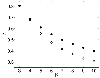
Figure 2: Static $\gamma_{c}$ (circles) and dynamic $\gamma_{d}$ (diamonds) transition for positive 1-in-K SAT for various values of $K$.

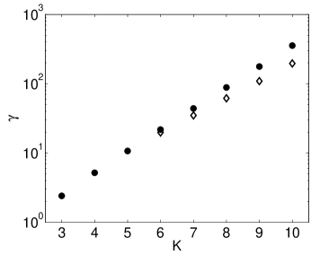
Figure 3: Static $\gamma_{c}$ (circles) and dynamic $\gamma_{d}$ (diamonds) transition for positive K-NAE SAT for various values of $K$.

In Fig. 5 we plot time variations of the landscape parameters, $M_{m}=M_{\ast m}$, corresponding to the global minimum of the effective potential. In Fig. 5 we plot a time-variation of the scaled ground-state energy $g$ given by the value of the effective potential at its minimum. Singular behavior corresponding to the first-order quantum phase transition at certain $\tau=\tau_{*}$ ($\Gamma=\Gamma_{*}$) can be clearly seen from the figures. Plots in Figs. 5 and 5 correspond to precisely the static transition $\gamma=\gamma_{c}$ for the case of $K=4$ in 1-in-K SAT problem.

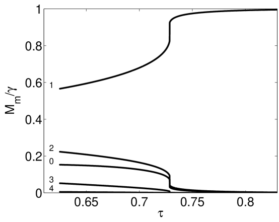
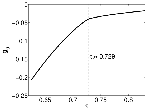
Figure 4: Plots of the landscape parameters $M_{m}=M_{\ast m}$ at the global minimum of the effective potential, vs $\tau$ for $K=4$ and $\gamma=\gamma_{c}$ (1-in-K SAT problem). Curves labeled 0-4 correspond to $M_{\ast 0}/\gamma$ through $M_{\ast 4}/\gamma$.

Figure 5: Scaled energy of adiabatic ground state $g_{0}$ vs $\tau$

for K=4 and $\gamma=\gamma_{c}$ (1-in-K SAT problem).

In the region $\gamma_{d}<\gamma<\gamma_{c}$ there are exponential (in $N$) number of solutions to Satisfiability problem but the runtime of the quantum adiabatic algorithm to find any of them also scales exponentially with $N$. This is a hard region for this algorithm. We note, that in the limit of $K\to\infty$ the annealing approximation becomes exact. Together with the fact that for large $K$ $\gamma_{d}$ and $\gamma_{c}$ seem to be distinctly different provides evidence that this result (existence of hard region for quantum adiabatic algorithm) is robust.

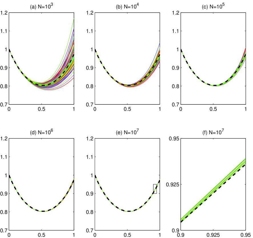
Figure 6: Results of numerical simulations and their comparison with theory. Depicted are Laplace transforms of ${\cal M}_{1}$ for 1-in-3 SAT. Numerical results: curves that have different colors correspond to different random problem instances; curves of same color correspond to different random bit strings. The dashed black line is a theoretical result based on the annealing approximation. The insets (a)-(e) depict instances with $10^{3}$, $10^{4}$, $10^{5}$, $10^{6}$, and $10^{7}$ binary variables. Since the error is not recognizable we replot in (f) a magnified section of inset (e). The bit strings were sampled with $q=0.422$, $M_{0}=0.048$, $M_{1}=0.416$, $M_{2}=0.123$, $M_{3}=0.013$, corresponding to $M/N=0.6$. These values correspond to the energy $E_{\infty}/2$ and they are shifted by 10% from the most likely values of $q,\{M_{m}\}$ for this energy (this shift is $\gg N^{1/2}$). We also note that for 1-in-3 SAT numerical simulations give static phase transition at $\gamma_{c}\approx$ 0.63).

VI Universality property for transition probabilities

Here we study the universal features of the transition probability in (10) for the set of macroscopic variables corresponding to the (normalized) total Ising spin $q$ and numbers of clauses of different types $\{M_{m}\}$ (38) (the type of a clause is equal to the number of unit bits involved in the clause). For simplicity, we shall focus in this section on the case $K=3$ only.

To clarify the above choice of macroscopic variables we consider an auxiliary quantity: a conditional probability distribution of the macroscopic variables $(q,\{M_{m}\})$ over the set of all possible configurations ${\boldsymbol{\sigma}}$ obtained by flipping $r$ bits of the configuration ${\boldsymbol{\sigma}}^{\prime}$. The first moments of this distribution corresponding to $M_{m}$,

$$\mu_{m}=\binom{N}{r}^{-1}\sum_{{\boldsymbol{\sigma}}}\delta\left[d({\boldsymbol{\sigma}}^{\prime}-{\boldsymbol{\sigma}}),\,r\right]\,M_{m}({\boldsymbol{\sigma}},{\cal I}),\quad m=0,\ldots,K,$$ (71)

can be easily computed by counting the number of ways one can flip $r$ bits in configuration ${\boldsymbol{\sigma}^{\prime}}$ to transform a $K$-bit clause of $m^{\prime}$ type (i.e., with $m^{\prime}$ unit bits) into a clause of the $m$-th type

$$\mu_{m}=\binom{N}{r}^{-1}\sum_{p,m^{\prime}=0}^{K}M_{m^{\prime}}\,\binom{m^{\prime}}{p}\binom{K-m^{\prime}}{m-m^{\prime}+p}\binom{N-K}{r-2p-m+m^{\prime}},$$ (72)

(here we use the convention $\binom{n}{m}\equiv 0$ for $m<0$ and $m>n$). In the double sum above values of ${\cal M}_{m^{\prime}}$ are multiplied by the number of possible ways to flip three groups of bits: $p$ unit bits in a clause of $m^{\prime}$-type, $p+m-m^{\prime}$ zero bits of this clause, and $r-2p-m+m^{\prime}$ bits of the configuration ${\boldsymbol{\sigma}}^{\prime}$ that do not belong to the clause. Similarly, one can show that the first moment corresponding to the variable $q$ equals $q^{\prime}(1-2r/N)$. It is clear that dependence of the first moments on the ancestor configuration ${\boldsymbol{\sigma}^{\prime}}$ is only via the variables $q^{\prime},\,M_{m}^{\prime}$ for that configuration.

In the limit, $r\gg 1$, the above conditional distribution has a Gaussian form with respect to $q$ and $M_{m}$. Elements of the covariance matrix $\Sigma_{m\,q}^{m^{\prime}\,q^{\prime}}({\boldsymbol{\sigma}^{\prime}})={\cal O}(r)$, and correspondingly, the characteristic width of the distribution is ${\cal O}(r^{1/2})$. For a configuration ${\boldsymbol{\sigma}^{\prime}}$ randomly sampled in the box $(q,\{M_{m}\})$ the r.m.s. deviation of the elements of $\Sigma_{m\,q}^{m^{\prime}\,q^{\prime}}({\boldsymbol{\sigma}^{\prime}})$ from their mean values in the box is ${\cal O}(N^{1/2})$. It is clear that in the limit $r\gg N^{1/2}$ the covariance matrix elements can be replaced by their mean values for the macroscopic state $(q,\{M_{m}\})$. Therefore in this limit the conditional distribution after $r$ spin flips starting from some macroscopic state depends only on the values of $(q,\{M_{m}\})$ in this state (universality property).

One can show that for $r\ll N^{1/2}$ the conditional distribution after $r$ spin flips can be expressed via the distribution (10) with $r=1$, using a standard convolution rule. Implicit in our derivation of landscapes is the relation between $r=1$ landscapes and a set of quantities $\{c_{\sigma,{\bf k}}\}$. Universality of landscapes should be interpreted as the fact that $\{c_{\sigma,{\bf k}}\}$ are self-averaging. Had we included only the energy instead of a full set of parameters, we would not have expected to see such self-averaging in the so-called replica-symmetry-broken phase. It is possible that inclusion of the full set of landscape parameters assures universality. We performed a series of numerical studies to test this hypothesis. In Figure 6 we present the results of numerical simulations and the comparison with analytic results within the annealing approximation. One can see that the property of self-averaging holds and that even annealing approximation provides very good description.

VII Random graph ensembles with reduced fluctuations

One can easily point out to a major deficiency of the annealing approximation – the fact that it fails to correctly predict the satisfiability transition. While part of it can be attributed to the fact that real entropy is slightly different from what is predicted by annealing approximation, major source of error is the incorrect assumption that the entropy vanishes at the satisfiability transition. That the entropy does not vanish can be easily seen by examining the structure of the random graph. At any finite connectivity (above percolation) it consists of one giant component and a large ${\cal O}(N)$ number of small ${\cal O}(1)$ components. Each small component contributes ${\cal O}(1)$ contribution to the entropy for a total of ${\cal O}(N)$ contribution, hence the entropy is in fact positive at all connectivities, including the satisfiability threshold.

VII.1 Concept of a core

An improvement over annealing bound for satisfiability threshold is possible. Note that clauses outside of giant component do not affect satisfiability and hence can be disregarded. Similarly, one can identify irrelevant clauses and remove them. Irrelevant clauses are those that can be eliminated without changing the satisfiability of the entire problem. We shall illustrate the identification of irrelevant clauses based on local properties for positive $K$-NAE SAT and positive $1$-in-$K$ SAT.

VII.1.1 Positive $K$-NAE SAT

For $K$-NAE SAT we can identify variables that do not enter any clause and remove them without affecting the satisfiability of the formula. Any variable that appear in exactly one clause can also be eliminated together with such clause, since the value of that variable can be adjusted to satisfy that clause. As one removes such clause, other variables may become candidates for removal. One can write an algorithm that iteratively removes variables that appear in no or exactly one clauses until no such variables remain (see Fig. 7). In fact using such algorithm improves running time of classical algorithm. The cost of this additional preprocessing is negligible: by using special data structures this algorithm can be made to run in $O(N\ln N)$ time.

It is not surprising that the result of running such trimming algorithm is a set of clauses and variables with a condition that every variable appears in at least two clauses. However, the statistical properties of the remaining core are not immediately apparent. As a first step, observe that the resulting core is independent of the order in which clauses and variables were removed. Hence we can study one specific algorithm.

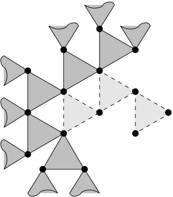
Figure 7: Example of trimming algorithm for 3-NAE SAT. Variables are represented graphically as vertices and clauses are represented as triangles. Incomplete triangles represent connections to the remainder of the graph (not shown). Shaded clauses are removed by the trimming algorithm.

First, we eliminate all variables of degree $0$ (that appear in no clauses). In the initial problem all instances with $N$ variables and $M$ clauses were equally probable. The number of vertices of degree $0$, $N_{0}$ does fluctuate, but for every specific value of $N_{0}$ all instances with $N-N_{0}$ variables, and $M$ clauses, and the additional property that each variable appear in at least one clause, are equiprobable. This property is referred to as uniform randomness. As a next step, identify variables of degree $1$ (appearing in exactly one clause). Although their number $N_{1}$ also fluctuates, for any fixed $N_{1}$, $N$ and $M$ all instances with $N$ variables of which $N_{1}$ variables have degree $1$ and $M$ clauses are equiprobable.

At each subsequent step of the algorithm we choose at random a variable of degree $1$ among $N_{1}$ candidates, and delete it together with the clause in which it appears. If the degree of any other variable in that clause becomes $0$, it is also deleted. Some variables which had degree $2$ previously may become degree $1$ variables. Obviously $M^{\prime}=M-1$, but the values of $N^{\prime}$ and $N_{1}^{\prime}$ cannot be predicted. But since the variable chosen for deletion was chosen at random (among all degree $1$ variables), one can show that although the values of $N^{\prime}$ and $N_{1}^{\prime}$ cannot be predicted, for every fixed set of $\{N^{\prime},N_{1}^{\prime},M^{\prime}\}$ all instances are equiprobable.

At the end of the algorithm $N_{1}\equiv 0$, hence for fixed $N^{\prime}$, $M^{\prime}$, all instances with $N^{\prime}$ variables, $M^{\prime}$ clauses and the condition that each variable appear in at least two clauses are equiprobable. Since average changes in $N$, $N_{1}$ and $M$ at each step were ${\cal O}(1)$ and corresponding deviations were also ${\cal O}(1)$, after ${\cal O}(N)$ steps needed for completion of the algorithm, fluctuations in resulting $N^{\prime}$ and $M^{\prime}$ are only ${\cal O}(\sqrt{N})$ by central limit theorem and can be neglected in our analysis.

There are several methods to derive the average resulting values of $N^{\prime}$, $M^{\prime}$. The most straightforward is to study the evolution of $N$, $N_{1}$ and $M$ by solving differential equations for their average values. This is somewhat tedious and less general. We instead resort to a different method of self-consistency equations. For every instance one can identify a set ${\cal C}$ of variables that form a core, i.e. those that will not be delete by the trimming algorithm. We now extend that set to ${\cal C}^{\prime}$ using the following rules:

1. If a variable belongs to ${\cal C}$, it also belong to ${\cal C}^{\prime}$.

2. If $K-1$ variables in some clause belong to ${\cal C}^{\prime}$, then the remaining variable must also belong to ${\cal C}^{\prime}$.

The minimal set ${\cal C}^{\prime}$ is obtained from ${\cal C}$ by iteratively adding variables according to these rules. Let the number of variables in set ${\cal C}^{\prime}$ be equal to $qN$ with $q<1$. Fluctuations in $q$ are $O(1/\sqrt{N})$ and, consequently, are neglected.

Now introduce $(N+1)$-st variable and compare systems with $N$ variables and $N+1$ variables. Together with $(N+1)$-st variable introduce $\Delta M$ clauses each involving that variable and $(K-1)$ random variables. The number $\Delta M$ is Poisson random variable with parameter $K\gamma$. We can compute the probability that the new variable belongs to ${\cal C}^{\prime}$ of the enlarged instance. The new variable belongs to ${\cal C}^{\prime}$ if for at least one of $\Delta M$ clauses, $K-1$ variables other than the new variables are not in ${\cal C}^{\prime}$ at the same time. Since these clauses are connected to random vertices, that probability can be expressed via $q$ alone and, owing to the fact that $\Delta M$ is Poisson, equals $1-\exp(-K\gamma q^{K-1})$. Self-consistency requires that this probability be equal to $q$:

$$1-q=e^{-K\gamma q^{K-1}}.$$ (73)

For practical purposes we must seek the largest solution to this equation.

Note that the new variable belongs to the core (set ${\cal C}$) if not for one, but for at least two of $\Delta M$ clauses, $K-1$ variables other than the new one are in ${\cal C}^{\prime}$. The probability of that

$$p=1-e^{-K\gamma q^{K-1}}-K\gamma q^{K-1}e^{-K\gamma q^{K-1}}\equiv q-K\gamma q^{K-1}(1-q)$$ (74)

is equal to the average value of $N^{\prime}/N$, and the average connectivity of the new vertex (under the condition that it is in ${\cal C}$) enables to compute $M^{\prime}/N^{\prime}$:

$$M^{\prime}/N^{\prime}=\frac{1}{K}\frac{K\gamma q^{K-1}\left(1-e^{-K\gamma q^{K-1}}\right)}{1-(1+K\gamma q^{K-1})e^{-K\gamma q^{K-1}}}\equiv\frac{\gamma q^{K}}{p}$$ (75)

(better expressed as $M^{\prime}/N=\frac{1}{K}K\gamma q^{K-1}\left(1-e^{-K\gamma q^{K-1}}\right)\equiv\gamma q^{K}$).

We must mention that the core for $K$-NAE SAT is in fact identical to that for $K$-XOR SAT. The latter has been analyzed by a different method Mezard:02 .

VII.1.2 Positive $1$-in-$K$ SAT

The situation is slightly more interesting in case of positive $1$-in-$K$ SAT. Setting a variable that appears in only one clause does not guarantee that the clause will be satisfied, hence the clause cannot be eliminated. Although it cannot be eliminated, it can still be simplified by eliminating the variable. The remaining instance will contain not only $K$-clauses but also one $(K-1)$-clause. The allowed combinations of variables for $(K-1)$-clauses should be those that have sum of variables equal to either $0$ or $1$. In that case the value of the deleted variable can always be adjusted so that the sum of variables in $K$-clause is exactly $1$.

Similarly, at some point $(K-1)$-clauses can be converted to $(K-2)$-clauses, $(K-3)$-clauses, down to $2$-clauses. In each case the allowed combinations shall have sum of spins either $0$ or $1$. Finally, if one can identify a variable that appears in $2$-clauses exclusively, this variable can be eliminated together with corresponding $2$-clauses, since setting it to $0$ shall satisfy all these clauses. As an illustration, see Fig. 8 which depicts $K=4$.

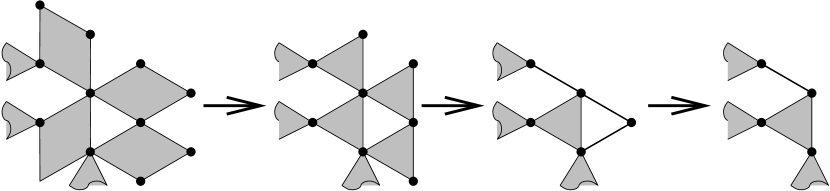
Figure 8: Example of trimming algorithm for 1-in-4 SAT. Variables are represented graphically as vertices and 4-, 3- and 2-clauses are represented as rhombi, triangles and edges correspondingly. Incomplete polygons represent connections to the remainder of the graph. The figure depicts evolution of part of the graph under trimming algorithm.

Once again, one can write trimming algorithm that eliminates such variables and clauses. As before, one can show that all remaining instances must have the property that each variable appear in at least two clauses of any length and at least one clause of length greater than two; and that for fixed number of vertices $N^{\prime}$, number of $2$-clauses $M_{2}^{\prime}$, …, $(K-1)$-clauses $M_{K-1}^{\prime}$, $K$-clauses $M_{K}^{\prime}$, all such instances are equiprobable.

Without going into details (available in our upcoming paper upcoming ), we should mention that equations now involve two variables $q$ and $q^{\prime}$, owing to separate treatment afforded to $2$-clauses and clauses of length greater than $2$. The self-consistency equations are:

$$1-q^{\prime} = e^{-K\gamma\left[1-(1-q)^{K-1}-(K-1)q(1-q)^{K-2}\right]},$$ (76)

$$1-q = (1-q^{\prime})e^{-K(K-1)\gamma q^{\prime}(1-q)^{K-2}},$$ (77)

with implicit understanding that the largest solutions $q$, $q^{\prime}$ are sought.

The expected values of $N^{\prime}$ as well as $M_{k}^{\prime}$ are given by

$$N^{\prime}/N = q^{\prime}-K\gamma\left[1-(1-q)^{K-1}-(K-1)q(1-q)^{K-2}\right](1-q),$$ (78)

$$M_{2}^{\prime}/N = \binom{K}{2}\gamma q^{\prime 2}(1-q)^{K-2},$$ (79)

$$M_{k}^{\prime}/N = \binom{K}{k}\gamma q^{k}(1-q)^{K-k}\quad{\rm for}k\geqslant 3.$$ (80)

Note that results for the core for positive $K$-NAE SAT and positive $1$-in-$K$ SAT allow for a compact formulation through introduction of generating function of allowed variable degrees.

For the case of $K$-NAE SAT it is $G(\mu)=\sum_{d\geqslant 2}\mu^{d}/d!=e^{\mu}-1-\mu$, since degrees of all variables are at least $2$. In terms of this $G(\mu)$, equations can be written as

$$N^{\prime}/N = e^{-\mu}G(\mu)$$ (81)

$$M^{\prime}/N = \frac{1}{K}\mu e^{-\mu}G^{\prime}(\mu)$$ (82)

with $\mu=K\gamma q^{K-1}$, and the equation on $q$ is

$$q=e^{-\mu}G^{\prime}(\mu).$$ (83)

For the case of $1$-in-$K$ SAT, $G$ is a function of $(K-1)$ variables reflecting the fact that the degree of each vertex is a vector $(d_{2},\ldots.,d_{K})$ where $d_{k}$ counts the number of appearances of said variable in $k$-clauses. The generating function for the remaining core is

$$G(\mu_{2},\mu_{3},\ldots,\mu_{K})=e^{\sum_{i=2}^{K}\mu_{i}}-e^{\mu_{2}}-\sum_{i=3}^{K}\mu_{i}.$$ (84)

There appears a set $\{q_{2},\ldots,q_{K}\}$ such that $q_{k}=(\partial/\partial\mu_{k})G(\{\mu_{i}\})$. Obviously, $q_{3}=q_{4}=\ldots=q_{K}$. Setting

$$\mu_{2} = 2\binom{K}{2}\gamma q^{\prime}(1-q)^{K-2},$$ (85)

$$\mu_{k} = k\binom{K}{k}\gamma q^{k-1}(1-q)^{K-k}\quad{\rm for}k\geqslant 3,$$ (86)

$N^{\prime}$ and $M_{k}^{\prime}$ can be compactly written as

$$N^{\prime}/N = e^{-\sum_{i=2}^{K}\mu_{i}}G(\{\mu_{i}\}),$$ (87)

$$M_{k}^{\prime}/N = \frac{1}{k}\mu_{k}e^{-\sum_{i=2}^{K}\mu_{i}}\frac{\partial}{\partial\mu_{k}}G(\{\mu_{i}\}).$$ (88)

VII.2 Improved annealing bound

Once irrelevant clauses have been removed we expect the entropy at the satisfiability transition to be much closer to zero. We have already made predictions for the number of remaining variables and clauses after trimming algorithm starting from a random graph of connectivity $\gamma$. We can compute the entropy of the remaining core. Using the critical connectivity at which the annealed entropy of the core alone becomes $0$ as an estimate of satisfiability transition is an improvement over traditional annealing approximation. We are motivated by two contributing factors: (i) the rigorous mathematical proof that the disorder is relevant for satisfiability transition relies on presence of irrelevant clauses, hence their removal can sometimes make disorder irrelevant, and (ii) applied to $K$-XOR SAT, this improved bound becomes exact Mezard:02 .

Doing annealing approximation on a core is hampered by the fact that clauses can no longer be assumed uncorrelated. However, the technique we introduced in this paper is well-suited for this example. The annealed entropy equals

$$s_{\rm ann}=\frac{1}{N^{\prime}}\ln{\cal N}(s,J)-\frac{1}{N^{\prime}}\ln{\cal N}(J),$$ (89)

where ${\cal N}(J)$ counts the number of possible disorders and ${\cal N}(s,J)$ is the total number of allowed spin-disorder configurations. We now separately consider $K$-NAE SAT and $1$-in-$K$ SAT.

VII.2.1 Positive $K$-NAE SAT

Consider the number of possible disorder realizations with $N^{\prime}$ variables, $M^{\prime}$ clauses with the constraint that each variable appear in at least two clauses. Each variable can be characterized by the vector ${\bf k}$ with $K$ components, each component $k_{p}$ counting the number of clauses where said variable appears in $p$-th position. Treating disorders that differ by permuting different clauses or permuting variables within a clause as different and fixing the fractions of vertices with particular realization of ${\bf k}$ to $c_{\bf k}$, the normalized logarithm of the count of possible disorders is

$$\frac{1}{N^{\prime}}\ln{\cal N}(J)\equiv s_{0}^{\prime}[N^{\prime},M^{\prime};\{c_{\bf k}\}]=-\sum_{\bf k}c_{\bf k}\ln\left[c_{\bf k}\prod_{p}k_{p}!\right]+K\frac{M^{\prime}}{N^{\prime}}\ln M^{\prime}.$$ (90)

We must maximize this expression with respect to $c_{\bf k}$ subject to constraints

$$\sum_{\bf k}k_{p}c_{\bf k}=M^{\prime}/N^{\prime}$$ (91)

and that $c_{\bf k}=0$ for $\sum_{p}k_{p}<2$.

Introducing Lagrange multipliers $\mu_{p}$, the expression for $c_{\bf k}$ becomes

$$c_{\bf k}=\frac{1}{G(\sum_{p}\mu_{p})}\prod_{p}\frac{\mu_{p}^{k_{p}}}{k_{p}!}.$$ (92)

Echoing the constraint that $\sum_{p}k_{p}\geqslant 2$, the normalization factor is $G(\sum_{p}\mu_{p})$ where $G(x)=e^{x}-1-x$ – the familiar generating function of the core. Using dual transformation we can rewrite the entropy as

$$s_{0}^{\prime}[N^{\prime},M^{\prime}]=\min_{\mu_{p}}\left\{\sum_{p}(M^{\prime}/N^{\prime})\ln\frac{M^{\prime}/N^{\prime}}{\mu_{p}}+\ln G\left(\sum_{p}\mu_{p}\right)\right\}+\frac{KM^{\prime}}{N^{\prime}}\ln N^{\prime}.$$ (93)

Comparing this expression with Eq.() we observe that the minimum is achieved for $\mu_{p}=\frac{1}{K}\mu\equiv\gamma q^{K-1}$, $\gamma$ being the connectivity of untrimmed random graph.

Now we proceed to count all possible combinations of spin assignments and disorder realizations ${\cal N}(s,J)$. Corresponding entropy is in general a function of $\{{\cal M}_{\boldsymbol{\alpha}}^{\prime}\}$ where ${\cal M}_{\boldsymbol{\alpha}}^{\prime}$ is the number of clauses with variables having values described by a vector $\{\alpha_{p}\}\equiv{\boldsymbol{\alpha}}$, divided by $N^{\prime}$ so that $\sum_{\boldsymbol{\alpha}}{\cal M}{\boldsymbol{\alpha}}=M^{\prime}/N^{\prime}$. In complete analogy with results of section V.1 we obtain

$$s_{1}^{\prime}[N^{\prime},M^{\prime};\{{\cal M}_{\boldsymbol{\alpha}}^{\prime}\};\{c_{\sigma,{\bf k}}\}] = -\sum_{\sigma,{\bf k}}c_{\sigma,{\bf k}}\ln\left[c_{\sigma,{\bf k}}\prod_{p,{\bf\alpha}}k_{\boldsymbol{\alpha}}^{p}!\right]+(K-1)\sum_{\boldsymbol{\alpha}}{\cal M}_{\boldsymbol{\alpha}}^{\prime}\ln{\cal M}_{\boldsymbol{\alpha}}^{\prime}+\frac{M^{\prime}}{N^{\prime}}\ln\frac{M^{\prime}}{N^{\prime}}$$ (94)

$$+\frac{KM^{\prime}}{N^{\prime}}\ln N^{\prime}.$$

Optimizing this with respect to $c_{\sigma,{\bf k}}$ subject to familiar constraints

$$\sum_{\sigma,{\bf k}}k_{\boldsymbol{\alpha}}^{p}c_{\sigma,{\bf k}}={\cal M}_{\boldsymbol{\alpha}}$$ (95)

and the constraint that $c_{\sigma,{\bf k}}=0$ if $\sum_{p,{\boldsymbol{\alpha}}}k_{\boldsymbol{\alpha}}^{p}<2$, the expression can be equivalently rewritten as

$$s_{1}^{\prime}[N^{\prime},M^{\prime};\{{\cal M}_{\boldsymbol{\alpha}}^{\prime}\}] = \min_{\mu_{\boldsymbol{\alpha}}^{p}}\left\{\sum_{p,{\boldsymbol{\alpha}}}{\cal M}_{\boldsymbol{\alpha}}^{\prime}\ln\frac{{\cal M}_{\boldsymbol{\alpha}}^{\prime}}{\mu_{\boldsymbol{\alpha}}^{p}}+\ln Z[\{\mu_{\boldsymbol{\alpha}}^{p}\}]\right\}+\frac{M^{\prime}}{N^{\prime}}\ln\frac{M^{\prime}}{N^{\prime}}-\sum_{\boldsymbol{\alpha}}{\cal M}_{\boldsymbol{\alpha}}^{\prime}\ln{\cal M}_{\boldsymbol{\alpha}}^{\prime}$$ (96)

$$+\frac{KM^{\prime}}{N^{\prime}}\ln N^{\prime},$$

with $Z[\{\mu_{\boldsymbol{\alpha}}^{p}\}]$ given instead by

$$Z[\{\mu_{\boldsymbol{\alpha}}^{p}\}]=G\left(\sum_{p,{\boldsymbol{\alpha}}}\delta[\alpha_{p};1]\mu_{\boldsymbol{\alpha}}^{p}\right)+G\left(\sum_{p,{\boldsymbol{\alpha}}}\delta[\alpha_{p};-1]\mu_{\boldsymbol{\alpha}}^{p}\right).$$ (97)

Labeling arguments by $\mu_{+}$ and $\mu_{-}$ respectively allows us to simplify this to

$$s_{1}^{\prime}[\{{\cal M}_{\boldsymbol{\alpha}}^{\prime}\}] = \min_{\mu_{\pm}}\left\{{\cal M}_{+}^{\prime}\ln\frac{{\cal M}_{+}^{\prime}}{\mu_{+}}+{\cal M}_{-}^{\prime}\ln\frac{{\cal M}_{-}^{\prime}}{\mu_{-}}+\ln[G(\mu_{+})+G(\mu_{-})]\right\}$$ (98)

$$+\frac{M^{\prime}}{N^{\prime}}\ln\frac{M^{\prime}}{N^{\prime}}-\sum_{\boldsymbol{\alpha}}{\cal M}_{\boldsymbol{\alpha}}^{\prime}\ln{\cal M}_{\boldsymbol{\alpha}}^{\prime}+\frac{KM^{\prime}}{N^{\prime}}\ln N^{\prime}.$$

with ${\cal M}_{+}^{\prime}=\sum_{{\boldsymbol{\alpha}}}\left(\sum_{p}\delta[\alpha_{p};1]\right){\cal M}_{{\boldsymbol{\alpha}}}^{\prime}$ and ${\cal M}_{-}^{\prime}=\sum_{{\boldsymbol{\alpha}}}\left(\sum_{p}\delta[\alpha_{p};-1]\right){\cal M}_{{\boldsymbol{\alpha}}}^{\prime}$.

The correct annealed entropy is given by the difference of these expressions

$$s_{{\rm ann}}^{\prime}[N^{\prime},M^{\prime};\{{\cal M}_{\boldsymbol{\alpha}}^{\prime}\}]=s_{1}^{\prime}[N^{\prime},M^{\prime};\{{\cal M}_{{\boldsymbol{\alpha}}}^{\prime}\}]-s_{0}^{\prime}[N^{\prime},M^{\prime}]$$ (99)

This enables us to find the improved bound on satisfiability threshold (where $H_{{\rm ann}}=0$) or to compute the most likely values of $\{{\cal M}_{{\boldsymbol{\alpha}}}^{\prime}\}$ for particular energy $E$.

Note that for positive $K$-NAE SAT corrections to static threshold due to this improved approximation are minute, since the transition happens at large connectivities, where simple annealing approximation adequately describes the transition.

VII.2.2 Positive $1$-in-$K$ SAT

For $1$-in-$K$ SAT the derivation is quite similar. An important addition is that the clauses can have any length from $2$ to $K$, hence index ${\bf k}$ should reflect that fact. Since calculations are similar in spirit, we shall only provide the results

$$s_{0}^{\prime}[N^{\prime},\{M_{k}^{\prime}\}]=\min_{\mu_{k}}\left\{k\frac{M_{k}^{\prime}}{N^{\prime}}\ln\frac{kM_{k}^{\prime}/N^{\prime}}{\mu_{k}}+\ln G(\{\mu_{k}\})\right\}+\sum_{k=2}^{K}\frac{kM_{k}^{\prime}}{N^{\prime}}\ln N^{\prime},$$ (100)

with $G(\{\mu_{k}\})=\exp\left(\sum_{k=2}^{K}\mu_{k}\right)-e^{\mu_{2}}-\sum_{k=3}^{K}\mu_{k}$, and

$$s_{1}^{\prime} = \min_{\mu_{k,\pm}}\left\{\sum_{k=2}^{K}\left({\cal M}_{k,+}^{\prime}\ln\frac{{\cal M}_{k,+}^{\prime}}{\mu_{k,+}}+{\cal M}_{k,-}^{\prime}\ln\frac{{\cal M}_{k,-}^{\prime}}{\mu_{k,-}}\right)+\ln[G(\{\mu_{k,+}\})+G(\{\mu_{k,-}\})]\right\}$$ (101)

$$+\sum_{k=2}^{K}\left[{\cal M}_{k}^{\prime}\ln{\cal M}_{k}^{\prime}-\sum_{{\boldsymbol{\alpha}}}{\cal M}_{k,{\boldsymbol{\alpha}}}^{\prime}\ln{\cal M}_{k,{\boldsymbol{\alpha}}}^{\prime}\right]+\sum_{k=2}^{K}\frac{kM_{k}^{\prime}}{N^{\prime}}\ln N^{\prime},$$

and the complete expression for the annealed entropy is

$$s_{{\rm ann}}^{\prime}[N^{\prime},\{{\cal M}_{k}^{\prime}\};\{{\cal M}_{k,{\boldsymbol{\alpha}}}^{\prime}\}]=s_{1}^{\prime}[\{{\cal M}_{k,{\boldsymbol{\alpha}}}^{\prime}\}]-s_{0}^{\prime}[N^{\prime},\{M_{k}^{\prime}\}].$$ (102)

The numerical predictions for the point where the entropy becomes zero are provided in Table 2.

VIII QAA algorithm on a core: extended landscapes

Once we have reexpressed the entropy on a reduced graph, it is only natural to implement the quantum adiabatic evolution directly on the reduced graph. Correspondingly, we shall need to recompute landscapes for the reduced graph.

VIII.1 Positive $K$-NAE SAT

This case entails least difficulty, since we can use same landscape parameters $\{{\cal M}_{\boldsymbol{\alpha}}^{\prime}\}$, the difference being the exclusion of total spin from the list of parameters. The central quantity–$\ell^{\prime}(\{{\cal M}_{{\boldsymbol{\alpha}}}^{\prime}\})$–is still expressed in a similar form:

$$\ell^{\prime}(\{{\cal M}_{\boldsymbol{\alpha}}^{\prime}\})=\sum_{\sigma,{\bf k}}c_{\sigma,{\bf k}}\exp\left[\frac{1}{2}\sum_{p,{\boldsymbol{\alpha}}}k_{\boldsymbol{\alpha}}^{p}\left(\frac{\partial s_{\rm ann}^{\prime}}{\partial{\cal M}_{\boldsymbol{\alpha}}^{\prime}}-\frac{\partial s_{\rm ann}^{\prime}}{\partial{\cal M}_{\bar{\boldsymbol{\alpha}}(p,{\boldsymbol{\alpha}})}^{\prime}}\right)\right].$$ (103)

Notably, the sum over ${\bf k}$ is now restricted to $|{\bf k}|\geqslant 2$. The derivatives of the entropy are still

$$\frac{\partial s_{\rm ann}^{\prime}}{\partial{\cal M}_{\boldsymbol{\alpha}}^{\prime}}=\sum_{p}\ln\frac{{\cal M}_{\boldsymbol{\alpha}}^{\prime}}{\mu_{\boldsymbol{\alpha}}^{p}}-\ln{\cal M}_{\boldsymbol{\alpha}}^{\prime}.$$ (104)

For ${\boldsymbol{\alpha}}$, ${\boldsymbol{\alpha}}^{\prime}$ differing in exactly one position, we shall have

$$\frac{1}{2}\left(\frac{\partial s_{\rm ann}^{\prime}}{\partial{\cal M}_{\boldsymbol{\alpha}}^{\prime}}-\frac{\partial s_{\rm ann}^{\prime}}{\partial{\cal M}_{{\boldsymbol{\alpha}}^{\prime}}^{\prime}}\right)=\frac{1}{2}\ln\frac{\mu_{{\boldsymbol{\alpha}}^{\prime}}^{p}}{\mu_{\boldsymbol{\alpha}}^{p}}.$$ (105)

Next, using $c_{\sigma,{\bf k}}=\frac{1}{Z}(\mu_{\boldsymbol{\alpha}}^{p})^{k_{{\boldsymbol{\alpha}}}^{p}}/k_{{\boldsymbol{\alpha}}}^{p}!$, for $|{\bf k}|\geqslant 2$ and Eq. (42), we are able to write, in terms of generating function $G(\mu)$:

$$\ell^{\prime}(\{{\cal M}_{\boldsymbol{\alpha}}^{\prime}\})=\frac{2}{Z}G\left(\sum_{<{\boldsymbol{\alpha}},{\boldsymbol{\alpha}}^{\prime}>}\sqrt{\mu_{\boldsymbol{\alpha}}^{p}\mu_{{\boldsymbol{\alpha}}^{\prime}}^{p}}\right)$$ (106)

Substituting ${\cal M}_{\boldsymbol{\alpha}}^{\prime}/\mu_{\boldsymbol{\alpha}}^{p}={\cal M}_{\alpha_{p}}^{\prime}/\mu_{\alpha_{p}}$, we can rewrite this as

$$\ell^{\prime}(\{{\cal M}_{\boldsymbol{\alpha}}^{\prime}\})=\frac{2}{G(\mu_{+})+G(\mu_{-})}G\left(\sqrt{\frac{\mu_{+}\mu_{-}}{{\cal M}_{+}^{\prime}{\cal M}_{-}^{\prime}}}\sum_{<{\boldsymbol{\alpha}},{\boldsymbol{\alpha}}^{\prime}>}\sqrt{{\cal M}_{\boldsymbol{\alpha}}^{\prime}{\cal M}_{{\boldsymbol{\alpha}}^{\prime}}^{\prime}}\right).$$ (107)

Note that for the landscapes on the original graph without spin variable, this expression is valid with $G(\mu)$ redefined to be $G(\mu)=e^{\mu}$.

VIII.2 Positive $1$-in-$K$ SAT

The notion of landscape parameters has to be generalized, since clauses of any length can appear. Correspondingly, we choose a set $\{{\cal M}_{k,{\boldsymbol{\alpha}}}^{\prime}\}$ to serve as landscape parameters. In contrast to $K$-NAE SAT, we have a total of $\sum_{k=2}^{K}(k+1)=(K-1)(K-2)/2$ parameters (with symmetries of ${\cal M}_{k,{\boldsymbol{\alpha}}}^{\prime}$ taken into account).

The derivation of landscapes can be generalized to include several types of clauses. The final answer is itself a generalization of Eq. (65)

$$\ell^{\prime}(\{{\cal M}_{k,{\boldsymbol{\alpha}}}^{\prime}\})=\frac{2}{G(\{\mu_{k,+}\})+G(\{\mu_{k,-}\})}G\left(\left\{\sqrt{\frac{\mu_{k,+}\mu_{k,-}}{{\cal M}_{k,+}{\cal M}_{k,-}}}\sum_{<{\boldsymbol{\alpha}},{\boldsymbol{\alpha}}^{\prime}>}\sqrt{{\cal M}_{k,{\boldsymbol{\alpha}}}^{\prime}{\cal M}_{k,{\boldsymbol{\alpha}}^{\prime}}^{\prime}}\right\}\right).$$ (108)

As before $G(\{\mu_{k}\})=\exp\left(\sum_{i=2}^{K}\mu_{i}\right)-e^{\mu_{2}}-\sum_{i=3}^{K}\mu_{i}$.

We can exploit the symmetry of ${\cal M}_{k,{\boldsymbol{\alpha}}}^{\prime}$ to write

$$\sum_{<{\boldsymbol{\alpha}},{\boldsymbol{\alpha}}^{\prime}>}\sqrt{{\cal M}_{k,{\boldsymbol{\alpha}}}^{\prime}{\cal M}_{k,{\boldsymbol{\alpha}}^{\prime}}^{\prime}}=\sum_{m=0}^{k-1}\sqrt{(m+1)(k-m)M_{k,m}^{\prime}M_{k,m+1}^{\prime}}.$$ (109)

Same is possible for $K$-NAE SAT; in fact it is precisely this form that is used in numerical calculations.

VIII.3 Numerical Results

Here we provide the numerical results for the satisfiability transition as determined by maximizing the entropy for energy $E=0$ and solving $s_{\rm ann}^{\prime}=0$. And we also list the location of dynamical transition, indicated by global bifurcation in $f^{\prime}=\varepsilon^{\prime}-\Gamma\ell^{\prime}$. All results are expressed in terms of connectivity of the original random graph for easy comparison with Table 1.

We observed that this refinement of our analysis leaves $\gamma_{d}$ and $\gamma_{c}$ of $K$-NAE SAT essentially unchanged. This is the manifestation of the fact that if either $K$ or $\gamma$ is large, the core is not much different from the original graph (i.e. that $q\approx 1$). In contrast, the difference for $1$-in-$K$ SAT is quite perceptible. For consistency, we compare the location of dynamic phase transition computed on the core to that computed on the original graph using only ${M_{m}}$ as landscape parameters (omitting total spin, as it is not among parameters for computations performed on a core). We also include new better bounds on static transition. All results are summarized in Table 2 and Fig. 9.

	K	3	4	5	6	7	8	9	10
Improved	$\gamma_{d}^{\prime}$	–	–	0.535	0.469	0.421	0.379	0.344	0.317
	$\gamma_{c}^{\prime}$	0.653	0.609	0.553	0.507	0.468	0.435	0.407	0.382
Old	$\gamma_{d}$	–	0.671	0.552	0.471	0.413	0.368	0.333	0.304
	$\gamma_{c}$	0.805	0.676	0.609	0.548	0.500	0.461	0.428	0.400

Table 2: Dynamic and static transition for positive $1$-in-$K$ SAT with improved annealing approximation and with old method using $\{M_{m}\}$ as landscape parameters. Prediction of $\gamma_{c}^{\prime}$ for $K=3$ compares favorably with result of simulations of $\gamma_{c}^{\prime}\approx 0.63$. No value (–) indicates the ebasence of dynamical transition.

Figure 9: Static (circles) and dynamic (diamonds) transition for various values of $K$ for positive $1$-in-$K$ SAT.

IX Conclusion

We have formulated an ansatz of landscapes and studied the complexity of the quantum adiabatic algorithm within the annealing approximation and found the existence of a dynamic transition and a hard(exponential) region above that dynamic transition. However, a similar analysis of simulated annealing did not reveal any phase transitions. We explain this as follows. The annealing approximation should fail for sufficiently small energies. It is commonly known that simulated annealing can find suboptimal solutions with very small energies very efficiently, but it takes an exponentially long time to actually reach the ground state. The annealing approximation does not correctly describe very small energies and cannot be used to establish its complexity. Note that we can reconcile this with the fact that the annealing approximation becomes exact in the limit when number of bits in a clause $K\to\infty$: if the annealing approximation fails for some $E\lesssim E_{K}$ we expect that $E_{K}$ is decreasing to zero as $K$ increases. However for any finite $K$, the free energy computed within the annealing approximation is free from any singularities indicative of a phase transition. To study the complexity of simulated annealing one needs to use the tools of spin glass theory, in particular, the replica trick SGTB ; Monasson:prl96 ; Monasson:pre97 (see also below).

In contrast, in our analysis of the quantum adiabatic algorithm, we observed a first-order phase transition, and, importantly, it happens for energies $E_{*}=O(E_{\infty})$ (where $E_{\infty}$ is the expected energy at infinite temperature, $E_{\infty}=\frac{1}{2^{n}}\sum_{z}E_{z}$). Moreover, the energies on both sides of the transition, relative to $E_{\infty}$ seem not to change appreciably with increasing $K$. Since the annealing approximation for this range of energies can be used, the prediction for the dynamic transition should survive, though the exact numerical values may acquire corrections. We have recomputed the dynamic transition with simplified energy-only landscapes (see Fig. 10). For 1-in-K SAT one can clearly see that the relative correction quickly diminishes. We believe that same happens for K-NAE SAT if sufficiently large $K$’s are considered. If this indeed holds, it serves as a corroboration that our results are correct numerically for large $K$. It should be noted that the large-K limit corresponds to the so-called random energy model, where one does not expect to perform better then ${\cal O}(2^{N})$ via any quantum algorithm.

The idea of using energy-only landscapes was present in Hogg:01 as well as Macready and Smel . A jump in the time-dependence of the expected energy value was seen in numerical simulations Hogg:02 , indicative of first-order phase transition, though a different ensemble was considered (only instances having a unique solution were considered).

We also attempted to go beyond simple annealing approximation and studied the dynamical transition using its refinement. For that we developed a polynomial mapping of the optimization problem defined on a full graph onto the problem defined on its subgraph (a core) where disorder-related fluctuations are significantly reduced and annealing approximation is expected to perform much better. As a test we used annealing approximation on a core to calculate the position $\gamma_{c}$ of a static (satisfiability) transition where the entropy of the state with $E$=0 vanishes. We also computed $\gamma_{c}$ numerically and found it to be very close to the analytical result. We then studied the dynamics of quantum adiabatic evolution algorithm on a core using an extended set of landscape functions and found that old results obtained on a full graph are reproduced qualitatively. This supports our earlier prediction that the location of the phase transition is not very sensitive to exact nature of annealing approximation employed.

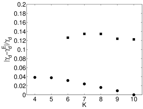
Figure 10: Relative difference between predictions for the dynamical phase transition point in the case of full ($\gamma_{d}$) and energy-only ($\gamma_{d}^{E}$) landscapes vs of $K$ for 1-in-K SAT (circles) and K-NAE SAT (squares).

We emphasize that different versions of annealing approximation employed in this paper describe the phase transition as a global bifurcation between two macroscopic states (pure states) in the space of macroscopic variables defined by a set of landscape functions. The complexity is due to tunneling between the pure states. In contrast, spin glass theory predicts the existence of an infinite number of pure states SGTB at sufficiently small energies. On the other hand, as we mentioned above the first-order quantum phase transition occurs for large energies $E_{*}$ and this has been confirmed with an improved annealing approximation.

Although the transition is seemingly absent for small $K$, a better approach (as compared to annealing approximation) may reveal it. Moreover, we believe that if this happens the order of the transition will remain unchanged, suggesting that the disorder may be irrelevant for the determination of the order of the phase transition and, consequently, for the complexity of the quantum adiabatic algorithm. That is, the exponential complexity is not due to the true combinatorial complexity of the underlying random optimization problem but rather due to peculiarities of the driver term and a particular ensemble of random instances considered.

A future extension of the present work is to include sufficiently large (possibly infinite) number of landscape parameters, thereby making annealing approximation increasingly precise. In this regard we recall that 1-bit-flip conditional distribution over landscape parameters employed in this paper (42) can be expressed via the set of coefficients $\{c_{\sigma,{\bf k}}\}$ that are concentrations of binary variables in a given string with different types ($\sigma,{\bf k}$) of an immediate neighborhood. In fact, these coefficients themselves can be used in an extended set of landscape parameters ${\bf x}$. Then appropriate effective potential $f({\bf x},\Gamma)$ can be introduced and its bifurcation can be studied when $\Gamma$ varies from $\infty$ to $0$. Furthermore, one can consider introducing progressively larger sets of landscape functions by defining neighborhoods of progressively larger size and using the well-known property that local structure of random (hyper)graph is tree-like cavity .

X Acknowledgments

This work was supported in part by the National Security Agency (NSA) and Advanced Research and Development Activity (ARDA) under Army Research Office (ARO) contract number ARDA-QC-P004-J132-Y03/LPS-FY2003, we also want to acknowledge the partial support of NASA CICT/IS program.

We would also like to acknowledge helpful comments by E. Farhi, J. Goldstone (MIT) and S. Gutmann (Northeastern U).

Appendix A On the NP-completeness of Positive $1$-in-$K$ Sat and
Positive $K$-NAE-Sat.

We set out to prove that both Positive $1$-in-$K$ Sat and $K$-NAE-Sat are NP-complete. It is straightforward to see that it takes a polynomial time to verify the assignment, so these problems are in NP. We now prove that they are as hard as the Satisfiability problem, which is NP-complete, by showing that any boolean formula can be represented as an instance of these.

A.1 Positive $1$-in-$K$ Sat

A clause of type $(x,\ldots,x,y)$ necessarily implies $x=0$ and $y=1$; hence we can represent constants $0$ and $1$. A clause of type $(0,\ldots,0,x,y)$ implies $x=\neg y$. Finally, a clause of type $(0,\ldots,0,x,y,z)$ is equivalent to a 3-clause $(x,y,z)$ so that we can restrict ourselves to $K=3$ without losing generality.

For $K=3$, immediately observe that three clauses $(x,z,u^{\prime})(y,z,u^{\prime\prime})(u,u^{\prime},u^{\prime\prime})$ with free variables $u,u^{\prime},u^{\prime\prime}$ implies $z=\neg(x\wedge y)$. This basic building block is in fact sufficient to build any boolean formula, as a result, any boolean formula can be cast as an $1$-in-$K$ SAT formula.

A.2 Positive $K$-NAE-Sat

A clause of type $(x,\ldots,x,y)$ necessarily implies $x=\neg y$, and $(x,\ldots,x,y,z)$ is equivalent to $(x,y,z)$ so we once again restrict ourselves to $K=3$. In contrast to $1$-in-$K$ problem, we shall require a non-trivial representation of false or true. We will use pairs of variables to denote variables of the boolean formula. Pairs $00$ or $11$ will represent value false and pairs $01$ or $10$ will represent true.

The next building block, $(x,y,t)(y,z,t)(z,x,t)$ ensures that $t=1$ if the majority of $x,y,z$ are $0$ and $t=0$ if the majority are $1$. We shall use a shorthand $f(t;x,y,z)$ to denote this. The expression $f(z_{1};x_{1},y_{1},y_{2})f(z_{2};x_{2},y_{1},y_{2})$ then ensures $z=x\wedge y$ where $x,y,z$ are represented as pairs $x_{1}x_{2}$, $y_{1}y_{2}$, $z_{1}z_{2}$ as indicated above. The operation of negation is trivial to represent: if $x\equiv x_{1}x_{2}$ then $\neg x\equiv(\neg x_{1})x_{2}$. These two are sufficient to construct any boolean formula.

Appendix B Next order approximation for landscapes

A better approximation for the values of critical clause-to-variable rations can be obtained if we specify the constraint that the distribution of vertex degrees be Poisson (as it is supposed to be in a random hypergraph Mezard:02 ). To be precise, we specify that

$$\sum_{\sigma,{\bf k}}c_{\sigma,{\bf k}}\prod_{p}\delta\left(\sum_{{\boldsymbol{\alpha}}}k_{{\boldsymbol{\alpha}}}^{p}-k_{p}\right)=c_{\{k_{p}\}}\equiv\frac{\prod_{p}\gamma^{k_{p}}}{\prod_{p}k_{p}!}e^{-\gamma K}.$$ (110)

Consequently, with this constraint the following expression for $c_{\sigma,{\bf k}}$ is obtained:

$$c_{\sigma,{\bf k}}=c_{\{k_{p}\}}\frac{e^{\lambda s}\prod_{p}\left[k_{p}!\prod_{{\boldsymbol{\alpha}}}(\mu_{{\boldsymbol{\alpha}}}^{p})^{k_{{\boldsymbol{\alpha}}}^{p}}/k_{{\boldsymbol{\alpha}}}^{p}!\right]}{Z_{\{k_{p}\}}},$$ (111)

where we use

$$Z_{\{k_{p}\}}=e^{\lambda}\prod_{p}\left(\sum_{\boldsymbol{\alpha}}\delta(\alpha_{p}-1)\mu_{{\boldsymbol{\alpha}}}^{p}\right)^{k_{p}}+e^{-\lambda}\prod_{p}\left(\sum_{\boldsymbol{\alpha}}\delta(\alpha_{p}+1)\mu_{{\boldsymbol{\alpha}}}^{p}\right)^{k_{p}}.$$ (112)

Annealed entropy can be rewritten in the form

$$s_{\rm ann}[q,\{{\cal M}_{{\boldsymbol{\alpha}}}\}]=\min_{\lambda,\mu_{{\boldsymbol{\alpha}}}^{p}}\left\{-\lambda q+\sum_{p,{\boldsymbol{\alpha}}}{\cal M}_{{\boldsymbol{\alpha}}}\ln\frac{{\cal M}_{{\boldsymbol{\alpha}}}}{\mu_{{\boldsymbol{\alpha}}}^{p}}+\ln Z[\lambda,\mu_{{\boldsymbol{\alpha}}}^{p}]\right\}-\sum_{{\boldsymbol{\alpha}}}{\cal M}_{{\boldsymbol{\alpha}}}\ln{\cal M}_{{\boldsymbol{\alpha}}}+\gamma\ln\gamma-\gamma K,$$ (113)

where $\ln Z$ is given by

$$\ln Z=\sum_{\{k_{p}\}}c_{\{k_{p}\}}\ln Z_{\{k_{p}\}}.$$ (114)

The equations relating $q,\{{\cal M}_{{\boldsymbol{\alpha}}}\}$ and $\lambda,\{\mu_{{\boldsymbol{\alpha}}}^{p}\}$ are given in (47),(48).

Similarly to Sec. V.2 we will use the notation (50). Since $\ln Z$ depends only on $\lambda$ and $\mu_{\pm}$, $\partial\ln Z/\partial\mu_{{\boldsymbol{\alpha}}}^{p}$ depends only on $\sigma_{p}$. Therefore, ${\cal M}_{{\boldsymbol{\alpha}}}/\mu_{{\boldsymbol{\alpha}}}^{p}={\cal M}_{\sigma_{p}}/\mu_{\sigma_{p}}$. Correspondingly,

$$s_{\rm ann}[q,\{{\cal M}_{{\boldsymbol{\alpha}}}\}] = \min_{\lambda,\mu_{\pm}}\left\{-\lambda q+{\cal M}_{+}\ln\frac{{\cal M}_{+}}{\mu_{+}}+{\cal M}_{-}\ln\frac{{\cal M}_{-}}{\mu_{-}}+\ln Z\right\}$$ (115)

$$-\sum_{{\boldsymbol{\alpha}}}{\cal M}_{{\boldsymbol{\alpha}}}\ln{\cal M}_{{\boldsymbol{\alpha}}}+\gamma\ln\gamma-\gamma K$$

For convenience, we introduce new variables

$$\mu_{\pm}=\mu\,e^{\pm h}.$$ (116)

We then readily obtain

$$\ln Z=\gamma\ln\mu+\sum_{k}c_{k}\ln[2\cosh(\lambda+kh)],$$ (117)

(where $k=\sum_{p}k_{p}$ and $c_{k}=\frac{(\gamma K)^{k}}{k!}e^{-\gamma K}$) and $\mu$ drops out of the expression for $s_{\rm ann}$ altogether:

$$s_{\rm ann}[q,\{{\cal M}_{\boldsymbol{\alpha}}\}] = \min_{\lambda,h}\left\{-\lambda q-({\cal M}_{+}-{\cal M}_{-})h+\sum_{k}c_{k}\ln[2\cosh(\lambda+kh)]\right\}$$

$$- \sum_{{\boldsymbol{\alpha}}}{\cal M}_{{\boldsymbol{\alpha}}}\ln{\cal M}_{{\boldsymbol{\alpha}}}+{\cal M}_{+}\ln{\cal M}_{+}+{\cal M}_{-}\ln{\cal M}_{-}+\gamma\ln\gamma-\gamma K.$$

It is easy to see from this expression what the equations for $\lambda,h$ are:

$$\sum_{k}c_{k}\tanh[\lambda+kh] = q,$$ (119)

$$\sum_{k}kc_{k}\tanh[\lambda+kh] = {\cal M}_{+}-{\cal M}_{-}.$$

We now turn our attention to the function $\ell(q,\{{\cal M}_{\boldsymbol{\alpha}}\})$ given by (42) with $\theta$ and $y_{\boldsymbol{\alpha}}$ evaluated from Eqs. (56),(58). The computation of $e^{y_{{\boldsymbol{\alpha}}}-y_{{\boldsymbol{\alpha}}^{\prime}}}$ yields

$$e^{y_{{\boldsymbol{\alpha}}}-y_{{\boldsymbol{\alpha}}^{\prime}}}=\left(\sqrt{\frac{{\cal M}_{+}}{{\cal M}_{-}}}\sqrt{\frac{\mu_{-}}{\mu_{+}}}\right)^{\sigma_{p}}\sqrt{\frac{{\cal M}_{{\boldsymbol{\alpha}}^{\prime}}}{{\cal M}_{{\boldsymbol{\alpha}}}}}.$$ (120)

Multiplied by $\mu_{{\boldsymbol{\alpha}}}^{p}$ this becomes

$$\mu_{{\boldsymbol{\alpha}}}^{p}\,e^{y_{{\boldsymbol{\alpha}}}-y_{{\boldsymbol{\alpha}}^{\prime}}}=\frac{\sqrt{{\cal M}_{{\boldsymbol{\alpha}}}{\cal M}_{{\boldsymbol{\alpha}}^{\prime}}}}{\sqrt{{\cal M}_{+}{\cal M}_{-}}}\mu.$$ (121)

The expression for $\ell(q,\{{\cal M}_{\boldsymbol{\alpha}}\})$ can be written in the form (cf. (60))

$$\ell(q,\{{\cal M}_{\boldsymbol{\alpha}}\})=\sum_{\{k_{p}\}}\frac{c_{\{k_{p}\}}}{Z_{\{k_{p}\}}}\sum_{\sigma,{\bf k}}^{\prime}e^{\lambda s+2xs}\prod_{p}\left[k_{p}!\prod_{{\boldsymbol{\alpha}}}(\mu_{{\boldsymbol{\alpha}}}^{p}e^{y_{{\boldsymbol{\alpha}}}-y_{{\boldsymbol{\alpha}}^{\prime}}})^{k_{\alpha}^{p}}/k_{\alpha}^{p}!\right],$$ (122)

with the internal sum running over ${\bf k}$ consistent with a set of $\{k_{p}\}$ (110). Substituting the quantities defined above this becomes

$$\ell(q,\{{\cal M}_{\boldsymbol{\alpha}}\})=\sum_{\{k_{p}\}}c_{\{k_{p}\}}\frac{\sum_{\sigma}\prod_{p}\left(\mu\,\sum_{\boldsymbol{\alpha}}\delta(\alpha_{p}-\sigma)\frac{\sqrt{{\cal M}_{{\boldsymbol{\alpha}}}{\cal M}_{{\boldsymbol{\alpha}}^{\prime}}}}{\sqrt{{\cal M}_{+}{\cal M}_{-}}}\right)^{k_{p}}}{Z_{\{k_{p}\}}}.$$ (123)

After some transformations we finally obtain

$$\ell(q,\{{\cal M}_{\boldsymbol{\alpha}}\})=\sum_{k}c_{k}\frac{\left(\frac{\sum_{<{\boldsymbol{\alpha}},{\boldsymbol{\alpha}}^{\prime}>}\sqrt{{\cal M}_{{\boldsymbol{\alpha}}}{\cal M}_{{\boldsymbol{\alpha}}^{\prime}}}}{\sqrt{{\cal M}_{+}{\cal M}_{-}}}\right)^{k}}{\cosh[\lambda+kh]}.$$ (124)

where $\lambda,\,h$ are given by (50),(119). Using symmetric ansatz (66) it is straightforward to calculate from (124) the restricted function $\bar{\ell}(q,\{{\cal M}_{m}\})$ (cf. (67)). We must note however, that although this represents a next-order improvement over annealing approximation, the relative changes in $\gamma_{c}$ and $\gamma_{d}$ computed with this improved approximation are nearly imperceptible ($\sim$ 10^-4).

References

- (1) E. Farhi, J. Goldstone, S. Gutmann, and M. Sipser, arXiv:quant-ph/0001106.
- (2) E. Farhi, J. Goldstone, S. Gutmann, J. Lapan, A. Lundgren, and D. Preda, Science 292, 472 (2001).
- (3) T. Hogg, arXiv:quant-ph/0206059.
- (4) S. Lloyd, Science 273, 1073 (1996).
- (5) W.M. Kaminsky and S. Lloyd, in “Quantum Computing & Quantum Bits in Mesoscopic Systems” (Kluwer Academic, 2003), see also arXiv:quant-ph/0211152.
- (6) R.M. Karp, in R.E. Miller and J.W. Thatcher, eds. Complexity of Computer Computations, Plenum Press, New York, 1972, pp. 85-103.
- (7) A.M. Childs, E. Farhi, J. Goldstone, and S. Gutmann, arXiv:quant-ph/0012104.
- (8) Y. Boufkhad, V. Kalapala, and C. Moore, ”The Phase Transition in Positive 1-in-3 SAT”, to be published.
- (9) G. Semerjian and R. Monasson, Phys. Rev. E 67, 066103 (2003).
- (10) P. Cheeseman, B. Kanefsky and W.M. Taylor, Proc. of the International Joint conference on Artificial Intelligence, 1, pp. 331-337 (1991).
- (11) S. Kirkpatrick, B. Selman, Science 264, 1297 (1994).
- (12) Artificial Intelligence 81 (1-2) (1996), special issue on Topic, ed. by T. Hogg, B.A. Huberman, and C. Williams.
- (13) W.Barthel, A.K. Hartmann, and M. Weigt, Phys. Rev. E 67, 066104 (2003).
- (14) A. Messiah “Quantum Mechanics”, vol. 1 (North-Holland, 1966).
- (15) E. Farhi, J. Goldstone, S. Gutmann, arXiv:quant-ph/0201031.
- (16) W. Van Dam, M. Mosca, U. Vazirani, arXiv:quant-ph/0206003.
- (17) E. Farhi, J. Goldstone, S. Gutmann, arXiv:quant-ph/0208135.
- (18) A. Boulatov, V.N. Smelyanskiy, Phys. Rev. A 68, 062321 (2003); also arXiv:quant-ph/0309150.
- (19) R. Monasson and R. Zecchina, Phys. Rev. Lett 76, 3881 (1996).
- (20) R. Monasson and R. Zecchina, Phys. Rev. E 56, 1357 (1997).
- (21) M. Mezard, F. Ricci-Tersenghi, R. Zecchina, arXiv:cond-mat/0207140.
- (22) S. Knysh, V. Smelyanskiy, and R.D. Morris, in preparation (2004).
- (23) M. Mezard, G. Parisi and M.A. Virasoro, eds., Spin Spin Glass Theory and Beyond (World Scientific, Singapore, 1987).
- (24) T.Hogg, Phys. Rev. A 61, 052311-1 (2000).
- (25) W. Macready, unpublished.
- (26) V. Smelyanskiy, U. Toussaint, D. Timucin, arXiv:quant-ph/0202155.
- (27) M. Mezard, G. Parisi, arXiv:cond-mat/0207121.