Non-gaussian statistics from individual pulses of squeezed light

Abstract

We describe the observation of a “degaussification” protocol that maps individual pulses of squeezed light onto non-Gaussian states. This effect is obtained by sending a small fraction of the squeezed vacuum beam onto an avalanche photodiode, and by conditioning the single-shot homodyne detection of the remaining state upon the photon-counting events. The experimental data provides a clear evidence of phase-dependent non-Gaussian statistics. This protocol is closely related to the first step of an entanglement distillation procedure for continuous variables.

Researches on novel schemes to perform quantum key distribution (QKD) are presently very active. In that field, lots of interest has arisen recently on the use of quantum continuous variables (QCV). For instance novel QKD schemes using the quadrature components of amplitude and phase modulated coherent states have been recently proposed prl and experimentally demonstrated GVAWBCG03 . It has been shown that such coherent state protocols are secure against individual gaussian attacks for any value of the line transmission GVAWBCG03 ; qic , and actually more general proofs are presently under study gc ; IVAC .

An important practical advantage of coherent states QKD is that it can in principle reach very high secret bit rates GVAWBCG03 . However, even in the best possible case, coherent states QKD will not do much better than photon-counting QKD gisin in terms of absolute distance, because of the exponential attenuation in optical fibers : at some point which is now somewhere between 10 and 100 km, one hits a limit where the transmitted secret data gets buried into errors of various origins, that range from detectors dark counts to imperfect data processing.

In order to qualitatively improve the situation, i.e. to go much beyond the attenuation length of a strand of fiber, a major challenge is to implement quantum repeaters qr , based upon entanglement distillation and (most likely) quantum memories. Ultimately, the secret qubits would be simply teleported to a remote place, with which shared entanglement has been established bennett . Looking now at entanglement distillation for QCV, a difficulty appears quickly : most (if not all) QCV transmissions so far are using light beams with gaussian statistics. However, it has been shown that it is not possible to distillate entanglement from a gaussian input to a gaussian output by gaussian means eisert1 ; cirac . One has to jump “outside” the gaussian domain, though it is possible to reach it back at the end, at least in an approximate way eisert2 .

In this letter, we experimentally implement a procedure which we call “degaussification”, that maps short pulses of squeezed light onto non-Gaussian states. This protocol is based upon a post-selection triggered by a photon-counting event and uses only simple linear optical elements. Extending this procedure to entangled EPR beams -which is fairly simple in principle- provides the first step of an entanglement distillation procedure as proposed in ref. eisert2 .

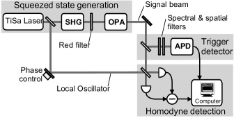
Figure 1: Simplified experimental setup

The experimental scheme is presented on Fig. 1. The initial pulses are obtained from a titanium-sapphire laser (Tiger-CD, Time-Bandwidth Products), delivering nearly Fourier-transform limited pulses at 850 nm, with a duration of 150 fs, an energy of 40 nJ, and a repetition rate of 790 kHz. These pulses are frequency doubled in a single pass through a thin (100 $\mu$m) crystal of potassium niobate (KNbO₃), cut and temperature-tuned for non-critical type-I phase-matching. The second harmonic power is large enough to obtain a significant single-pass parametric gain ($\sim$ 3 dB) in a similar KNbO₃ crystal used in a type-I spatially degenerate configuration.

Given this relatively high gain, “real” squeezed states are actually produced, not only parametric pairs. Therefore, higher order terms (beyond pair production) have explicitly to be included in the analysis as they play an essential role to understand the phase-dependence of the data. The detection scheme follows the basic idea of a pulsed squeezed light experiment laporta , with two important differences :

(i) All processing is done in the time domain, not in the frequency domain. For each incoming pulse, the balanced homodyne detection samples one value of the signal quadrature in phase with the local oscillator beam GVAWBCG03 . It is then possible to reconstruct the full statistics of the signal pulses. The histograms presented below are obtained from these individual pulse data.

(ii) A small fraction ($R=0.115$) of the squeezed vacuum beam is taken out from the homodyne detection channel. These trigger photons then pass through a spatial filter (made of two Fourier-conjugated pinholes) and a 3 nm spectral filter centered at the laser wavelength, before being detected by a silicon avalanche photodiode (APD). The detection click is registered simultaneously with the homodyne signal, and can be used to post-select homodyne events. As we will show, this selection provides directly non-gaussian statistics.

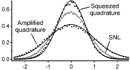
Figure 2: Normalized probability distribution for the (unconditioned) squeezed vacuum state, obtained from the pulsed homodyne detection. The squeezed quadrature variance is 1.75 dB below SNL, while the amplified quadrature variance is 3.1 dB above. The SNL curve corresponds to the vacuum state, where the shot noise variance is taken equal to 1/2.

The unconditioned distributions corresponding to the squeezed and anti-squeezed quadratures, and to the vacuum noise are plotted on fig. 2. More experimental details about the squeezed states generation will be given in another publication. The measured squeezing variance (with no correction) is 1.75 dB below the shot noise level (SNL), in good agreement with the measured deamplification of a probe beam (0.50 or 3 dB) and our evaluation of the overall detection efficiency $\eta_{tot}=\eta\;(1-R)=0.66$. Here $1-R=0.885$ is the transmission of the conditioning beamsplitter, and $\eta=0.75$ is the homodyne detection efficiency (see details below). As it can be seen on fig. 2, the experimental data for both quadratures is correctly fitted by assuming a single-mode parametric gain $\exp(\pm 2s)$ with $s=0.43$, together with the above efficiency $\eta_{tot}$. We note however that the deamplification gain of the probe beam does not correspond exactly to the inverse of the amplification, due to gain-induced-diffraction which distorts the probe phase fronts Gid . Since such multimode effects remain reasonably small in our experimental conditions, we will use the single parameter $s$ to describe parametric amplification and deamplification.

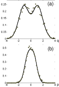
Figure 3: Experimental (dots) and theoretical (line) quadrature distribution of the post-selected homodyne measurements for the amplified quadrature (a) and the squeezed one (b), normalized as in fig. 2. Parameters used in the calculation are $s=0.43$, $R=0.115$, $\eta=0.75$ and $\xi=0.7$ .

Fig. 3 displays the post-selected output of the homodyne detection resulting from the degaussification protocol, showing a clear dip in the centre of the amplified quadrature distribution. The theoretical curves represented on the same figure are obtained from a simple single-mode model detailed below. This model takes into account the measured parametric gain, together with various experimental imperfections (losses, imperfect mode-matching, electronic noise, dark counts and modal purity, see below for details), and it is clearly in good agreement with the experimental data.

The origin of the observed effect can be analyzed in different ways. A first insight can be obtained by considering the homodyne detection of a conditional single photon state, observed in ek . In this experiment, the authors separate the two photons from a parametric pair, and one of them is used as a trigger on a photon counter, while the other one is sent to an homodyne detection. In the ideal case, such an experiment would measure the probability density $P(x)$ of the $n=1$ Fock state, which is non-gaussian since $P(0)=0$. Though this experiment provides a first idea of the origin of the non-gaussian features, it is not enough to explain our observations. Actually, we see phase-dependent effects (while a $n=1$ Fock state is phase-independent), and in our set-up there is no explicit separation of the photon pair.

We have carried out a calculation taking into account the expansion of the squeezed state in a Fock state basis, including terms up to $n=10$, which is enough for our degree of squeezing. The calculation is done for an arbitrary value of the conditioning beamsplitter reflectivity, and takes into account the various imperfections of the experiment. This calculation is straightforward but tedious, and one can actually get a good physical insight by considering the restricted simple case of an expansion of the squeezed vacuum up to $n=4$, and a beamsplitter reflectivity $r=\sqrt{R}\ll 1$. The squeezed vacuum $\mid\Psi_{s}\rangle$ can then be written as :

$$\mid\Psi_{s}\rangle=\alpha\mid 0\rangle+\beta\mid 2\rangle+\gamma\mid 4\rangle$$ (1)

With our degree of squeezing $s=0.43$, one has $\alpha=0.96$, $\beta=0.27$ and $\gamma=0.10$ ulf . This state then gets mixed with the vacuum at the beamsplitter, resulting in a two-mode entangled squeezed state. Denoting as $r,t$ the reflectivity and transmittance of the beamsplitter ($r^{2}+t^{2}=1$), the output state is :

$$\mid\Psi_{s,out}\rangle=\left(\alpha\mid 0\rangle_{1}+t^{2}\beta\mid 2\rangle_{1}+t^{4}\gamma\mid 4\rangle_{1}\right)\mid 0\rangle_{2}$$

$$+\left(\sqrt{2}rt\beta\mid 1\rangle_{1}+2rt^{3}\gamma\mid 3\rangle_{1}\right)\mid 1\rangle_{2}+O(2)$$ (2)

where $\mid.\rangle_{1}$ denotes the state sent to the homodyne detection, while $\mid.\rangle_{2}$ stands for the state sent to the APD. The term $O(2)$ denotes Fock state terms higher than 1 on the APD beam, which will be neglected in this simplified calculation, given our assumption $r\ll 1$. Finally, post-triggering on the APD photon-counting events reduces the state detected by the homodyne detection to :

$$\mid\Psi_{cond}\rangle\propto\beta\mid 1\rangle+\sqrt{2}\gamma\;t^{2}\mid 3\rangle$$ (3)

The prediction of this calculation is shown on fig. 4. As it could be expected, we do obtain phase-dependent non-gaussian statistics. These features are related to high order terms beyond pair production which play an essential role in our analysis.

In this simplified calculation we have assumed $r<<1$, and the predicted dip in the centre of the probability distribution goes down to zero. When the beamsplitter reflectivity is increased, Fock state terms with $n>1$ may no longer be neglected on the APD beam, and the central dip has a non-zero value. Strictly speaking, this is not an experimental imperfection, but an intrinsic feature of the conditioned state for larger $R$, which clearly appears on the result of the full calculation also displayed on Fig. 4.

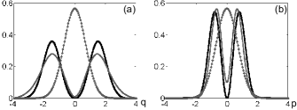
Figure 4: Phase-dependent quadrature distributions of the conditioned homodyne measurements, together with the vacuum reference (line and dots). The thick solid line is obtained from eq. (3) with $R=0.01$. The thin gray line is obtained from the complete calculation and $R=0.115$. Fig. (a) corresponds to the amplified quadrature while fig. (b) shows the squeezed one. The squeezing parameter is $s=0.43$, and perfect single mode detection efficiency has been assumed.

In order to characterize experimental imperfections, let us emphasize that the homodyne detection and the photon-counting detection have quite different drawbacks. The homodyne detection is not sensitive to “real” photons that are in modes unmatched with the detected (local oscillator) mode, but it is quite sensitive to vacuum modes which couple into this detected mode. On the other hand, the photon-counting detection is not sensitive to vacuum noise, but it will detect photons in any modes. Correspondingly, two experimental parameters must be used : an homodyne efficiency parameter $\eta$, which measures the overlap between the desired signal mode and the detected mode GG ; and a modal purity parameter $\xi$, which characterizes which fraction of the detected photons are actually in the desired signal mode KK . In the simplest approach, the homodyne efficiency can be modelized by a lossy beamsplitter, taking out desired correlated photons. On the other hand, the modal purity $\xi$ in our experiment cannot be modelized by another lossy beamsplitter, because a small value of $\xi$ corresponds to unwanted firings of the APD, for which a squeezed vacuum is still measured at the homodyne detection port. More precisely, the measured probability distribution for a quadrature $x$ will be taken as $P(x)=\xi\;P_{cond}(x)+(1-\xi)\;P_{uncond}(x)$, where $P_{cond}(x)$ and $P_{uncond}(x)$ are respectively the conditioned and unconditioned probability distributions, which depend on the values of $s$, $R$ and $\eta$.

It is then easy to determine values of the parameters $\eta$ and $\xi$ fitting the experimental data. The procedure to measure $\eta$ is well established from squeezing experiments laporta , and it can be cross-checked by comparing the classical parametric gain and the measured degree of squeezing. The procedure to measure $\xi$ is less usual, and amounts to evaluate how many unwanted photons make their way through the spatial and spectral filters which are used on the photon counting channel. Ultimately, this estimated value of $\xi$ must fit with the observed conditional probability distribution, since $\eta$ is independantly obtained from squeezing measurements.

Experimentally, this procedure turns out to be quite successful, and for instance we have plotted on fig. 3 the amplified and deamplified conditional probability distributions, using as parameters the parametric gain $\exp(2s)=2.36$, the homodyne efficiency $\eta=0.75$, and the modal purity parameter $\xi=0.7$. We note that the value of $s$ is evaluated from the measured squeezing (see fig. 2), while $\eta$ is obtained as $\eta=\eta_{T}\eta_{H}^{2}\eta_{D}$, where the overall transmission $\eta_{T}=0.94$, the mode-matching visibility $\eta_{H}=0.92$, and the detectors efficiency $\eta_{D}=0.945$ are independantly measured. Finally, the modal purity $\xi$ is fitted to the data, and cross-checked as the ratio between the expected and actual APD counting rates.

In a last step, we have analysed our data using the standard techniques of quantum tomography. We have recorded an histogram with 40 bins for 6 different quadrature phase values $\theta$, and about 5000 points for each histogram were acquired in a 3 hours experimental run. The Wigner function displayed on fig. 5 was then reconstructed using the Radon transform ulf , applied to the symetrized experimental data $(P(x_{\theta})+P(-x_{\theta}))/2$, without any correction for measurement efficiency. It shows a clear dip at the origin, with a central value of 0.067 while the maximum is at 0.12.

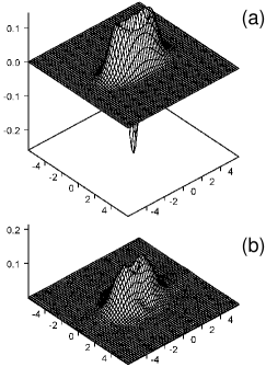
Figure 5: (a) Theoretical Wigner function $W$ of the output state of the “degaussification” protocol, assuming $s=0.43$, $R=0.115$ and perfect detection ($\eta=\xi=1$). (b) Reconstructed Wigner function from the experimental data ($\eta=0.75$, $\xi=0.7$). The values of $W$ at the origin of phase space are respectively $W_{th}(0,0)=-0.26$, and $W_{exp}(0,0)=0.067$.

As usual, the conditions to get negative values of the measured Wigner function are rather stringent, and require the presence of a dip into the distribution probability associated to the squeezed quadrature. Given our experimental parameters, this requires a modal purity $\xi$ better than $0.85$, which was not experimentally attainable while keeping the APD count rate above a few tens per second. Nevertheless, we point out that by correcting for the homodyne efficiency, the evaluated Wigner function of the prepared state (just before homodyne detection) does assume a negative value at the origin, $W_{cor}(0,0)\approx-0.06$. Another interesting feature is that the non-gaussian dip on the amplified quadrature is quite robust to losses and therefore can be easily observed with our experimental parameters. This is associated with a similarly robust “squeezed volcano shape” of the Wigner function.

We have described the first experimental observation of a “degaussification” protocol, mapping individual femtosecond pulses of squeezed light onto non-Gaussian states, by using only linear optical elements and an avalanche photodiode. The observed effect is closely related to the first step of an entanglement distillation procedure for gaussian quantum continuous variables eisert2 . This work should contribute to the future development of quantum repeaters and long-range quantum cryptography using continuous variables entanglement.

We thank F. Grosshans for his contribution to the early steps of the experiment, and J. Fiurášek for useful comments. This work was supported by the European IST/FET/QIPC program, and by the French programs “ACI Photonique” and “ASTRE”.

References

- (1) F. Grosshans and Ph. Grangier, Phys. Rev. Lett. 88, 057902 (2002).
- (2) F. Grosshans, G. Van Assche, J. Wenger, R. Brouri, N.J. Cerf and Ph. Grangier, Nature 421, 238 (2003).
- (3) F. Grosshans, N. J. Cerf, J. Wenger, R. Tualle-Brouri and Ph. Grangier, Quant. Inf. Comput. 3, 535 (2003).
- (4) F. Grosshans and N.J. Cerf, Phys. Rev. Lett. 92, 047905 (2004).
- (5) S. Iblisdir, G. Van Assche and N.J. Cerf, e-print quant-ph/0312018.
- (6) N. Gisin, G. Ribordy, W. Tittel, and H. Zbinden, Rev. Mod. Phys. 74, 145 (2002).
- (7) H.J. Briegel, W. Dur, J.I. Cirac and P. Zoller, Phys. Rev. Lett. 81, 5932 (1998).
- (8) C.H. Bennett et al , Phys. Rev. Lett. 70, 1895 (1993).
- (9) J. Eisert, S. Scheel and M.B. Plenio, Phys. Rev. Lett. 89, 137903 (2002).
- (10) G. Giedke and J.I. Cirac, Phys. Rev. A 66, 032316 (2002).
- (11) D.E. Browne, J. Eisert, S. Scheel and M.B. Plenio, Phys. Rev. A 67, 062320 (2003).
- (12) R.E. Slusher, P. Grangier, A. LaPorta, B. Yurke and M.J. Potasek, Phys. Rev. Lett. 59, 2566 (1987).
- (13) A. LaPorta and R.E. Slusher, Phys. Rev. A 44, 2013 (1991).
- (14) A.I. Lvovsky et al , Phys. Rev. Lett. 87, 050402 (2001).
- (15) F. Grosshans and P. Grangier, Eur. Phys. J. D. 14, 119 (2001).
- (16) T. Aichele, A.I. Lvovsky and S. Schiller, Eur. Phys. J. D. 18, 237 (2002).
- (17) U. Leonhardt, Measuring the quantum state of light (Cambridge University Press, Cambridge, 1997).