Generation of multi-photon Fock states by bichromatic adiabatic passage:
topological analysis

Abstract

We propose a robust scheme to generate multi-photon Fock states in an atom-maser-cavity system using adiabatic passage techniques and topological properties of the dressed eigenenergy surfaces. The mechanism is an exchange of photons from the maser field into the initially empty cavity by bichromatic adiabatic passage. The number of exchanged photons depends on the design of the adiabatic dynamics through and around the conical intersections of dressed eigenenergy surfaces.

I Introduction

Over the past few years, new sources of anti-bunched light that are able to emit a single photon in a given time interval has been the subject of an intense theoretical and experimental research. The driving force behind the development of these non-classical sources is a range of novel applications in quantum information theory which builds on the laws of quantum mechanics to transmit, store, and process information in varied and powerful ways. Advances in this field rely on the ability to manipulate coherently isolated quantum objects while eliminating incoherent interactions with the surrounding environment. Single photon states act as elementary quantum bits (qubits) in quantum cryptography Jennewein et al. (2000); Naik et al. (2000); Tittel et al. (2000) and teleportation of a quantum state Bouwmeester et al. (1997) where their entangled states enable secure transmission of information.

Many different types of single-photon sources have been proposed and realized using the controlled excitation of single molecules Brunel et al. (1999); Lounis and Moerner (2000) or of single nitrogen-vacancy centers in diamond nanocrystals Beveratos et al. (2002), controlled injection of carriers into a mesoscopic quantum well Kim et al. (1999) and using pulsed excitation of semiconductor quantum dots Santori et al. (2001); Michler et al. (2000).

In the context of cavity QED, single-photon Fock states have been produced by a Rabi $\pi$-pulse in a microwave cavity Maître et al. (1997); Varcoe et al. (2000) and by the STIRAP technique in an optical cavity Hennrich et al. (2000) based on the scheme proposed in Parkins et al. (1995) where the Stokes pulse is replaced by a mode of a high-Q cavity. The STIRAP process has also been studied in a system of four-level atom interacting with a cavity mode and two laser pulses, with a coupling scheme which generates two degenerate dark states Gong et al. (2002). In all these cavity QED schemes one atom interacts with a single-mode high-Q cavity and generates one photon. As the atoms pass through the cavity one by one, more photons can be added to the cavity. Recently another scheme has been proposed to generate a two-photon Fock state by a single two-level atom interacting with a superconducting cavity which sustains two non-degenerate orthogonally polarized modes Bertet et al. (2002). The photons are transferred from the source mode into the target mode of the cavity by a third-order Raman process. However this scheme is not robust relative to the velocity of atoms.

In this paper we propose a scheme in which a two-level atom interacts counterintuitively Vitanov et al. (2001) with a single-mode high-Q cavity and a delayed maser field that are both near-resonant with the atomic transition, allowing to produce a controlled number of photons in the cavity depending on the design of the adiabatic passage. This process is referred to as a bichromatic adiabatic passage since two near-resonant interacting fields act on a single transition. A related work involving exchange of photons between two laser fields through a bichromatic process can be found in Ref. Guérin et al. (2001). The transfer of photons from the maser field into the cavity field is based on the adiabatic passage between two dressed states which are the eigenstates of the coupled atom-maser-cavity system. This process is robust because it does not depend on the precise velocity of the atom or on the precise tuning of the maser and the cavity frequencies. The dynamics of the process, under the adiabatic conditions, can be described completely by the topology of the dressed eigenenergy surfaces. This topological aspect is the key to the robustness of the process. Our method is based on the calculation of the dressed eigenenergy surfaces of the effective Hamiltonian as a function of the two Rabi frequencies associated to the maser and the cavity fields, and the application of adiabatic principles to determine the dynamics of the process in view of the topology of the surfaces.

The paper is structured as follows. In Sec. II, we use the Floquet formalism and the phase representation of the creation and annihilation operators to construct the effective Hamiltonian of the atom-maser-cavity system. Eigenenergy surfaces of the effective Hamiltonian are displayed in Sec. III as a function of the normalized Rabi frequencies of the cavity and the maser fields. We demonstrate how the analysis of these surfaces allows to design different adapted adiabatic paths leading to different photon transfers into the cavity field without changing the atomic population at the end of the interaction. Sec. IV is devoted to the numerical simulation of the evolution governed by the effective Hamiltonian and the final probabilities of the one and two-photon transfer states. Finally, in Sec. V we give some conclusions and indicate conditions for experimental implementation.

II Construction of the effective hamiltonian

We consider a two-level atom of upper and lower states $|+\rangle$ and $|-\rangle$ and of energy difference $E_{+}-E_{-}=\omega_{0}$ as represented in Fig. 1. We use atomic units in which $\hbar=1$. The atom in its lower state is released from a source of atoms and falls through a high-Q cavity with velocity $v$. The atom first encounters the vacuum mode of the cavity with frequency $\omega_{C}$ and waist $W_{C}$ and then the maser beam with frequency $\omega_{M}$ and waist $W_{M}$. Both the maser and the cavity fields are near-resonant with the atomic transition. The distance between the crossing points of the cavity and the maser axis with the atomic trajectory is $d$. The travelling atom encounters time dependent and delayed Rabi frequencies of the cavity and the maser fields:

$$G(t) = -\mu\sqrt{\frac{\omega_{C}}{2\epsilon_{0}V_{\text{mode}}}}~{}~{}e^{-(\frac{vt}{W_{C}})^{2}},$$

$$\Omega(t) = -\mu\mathcal{E}_{M}~{}~{}e^{-(\frac{vt-d}{W_{M}})^{2}},$$ (1)

where $\mu$, $V_{\text{mode}}$, $\mathcal{E}_{M}$ are respectively the dipole moment of the atomic transition, the effective volume of the cavity mode and the amplitude of the maser field.

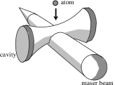
Figure 1: Experimental configuration and level scheme of the atom.

The detuning of the maser and the cavity fields from the atomic transition are $\Delta_{i}=\omega_{0}-\omega_{i},~{}~{}i=C,M$. We take the frequencies of the fields such that their difference $\delta=\omega_{C}-\omega_{M}$ is positive and very small with respect to $\omega_{C}$ and $\omega_{M}$. Also we assume

$$\text{max}\{|G(t)|~{},~{}|\Omega(t)|\}\ll\omega_{0}.$$ (2)

Under these conditions, the counter-rotating terms can be discarded in the rotating-wave approximation (RWA). The semiclassical Hamiltonian of the atom-maser-cavity system can thus be written as

$$H(t) = \omega_{C}a^{{\dagger}}a~{}\openone_{2}+\left(\begin{array}[]{cc}\omega_{0}&0\\ 0&0\\ \end{array}\right)+G(t)\left(\begin{array}[]{cc}0&a\\ a^{{\dagger}}&0\\ \end{array}\right)$$ (7)

$$+ \Omega(t)/2\left(\begin{array}[]{cc}0&e^{-i(\theta_{0}+\omega t)}\\ e^{i(\theta_{0}+\omega t)}&0\\ \end{array}\right),$$ (10)

where $a,a^{{\dagger}}$ are the annihilation and creation operators of the cavity field, $\openone_{2}$ is the $2\times 2$ identity matrix and the phase $\theta_{0}$ is the initial phase of the maser field. The energy of the lower atomic state has been taken as $0$. This Hamiltonian acts on the Hilbert space $\mathcal{H}\otimes\mathcal{F}$ where $\mathcal{H}=\mathbb{C}^{2}$ is the Hilbert space of the atom generated by $|\pm\rangle$ and $\mathcal{F}$ is the Fock space of the cavity mode generated by the orthonormal basis $\{|n\rangle~{};~{}n=0,1,2,\cdots\}$ with $n$ the photon number of the cavity field. The dynamics of system is determined by the Schrödinger equation

$$i\frac{\partial}{\partial t}\phi(t)=H(t)\phi(t),$$ (11)

where $\phi(t)\in\mathcal{H}\otimes\mathcal{F}$ with initial condition $\phi_{0}=\phi(t_{0})=|-\rangle\otimes|n=0\rangle$. We can think of Eq.(11) as a family of equations parameterized by the phase $\theta_{0}$. The time-dependent Hamiltonian (7) contains two different time scales: the period $T=2\pi/\omega$ characterizing fast oscillations of the maser field and $T_{int}\approx\frac{W_{M}}{v}\approx\frac{W_{C}}{v}$ characterizing the slow change of the field amplitudes $G(t),\Omega(t)$. The fast periodic time-dependence can be taken into account by use of Floquet theory. The evolution equation in the Floquet representation reads:

$$i\frac{\partial}{\partial t}\psi(t;\theta)=K(t;\theta)\psi(t;\theta),$$ (12)

where $\theta$ appears as a dynamical variable defined on the unit circle $\mathbb{S}^{1}$ of length $2\pi$, and $K(t;\theta)$ is the Floquet Hamiltonian

$$K(t;\theta) = \omega_{C}a^{{\dagger}}a~{}\openone_{2}+\left(\begin{array}[]{cc}\omega_{0}&0\\ 0&0\\ \end{array}\right)-i\omega_{M}\frac{\partial}{\partial\theta}~{}\openone_{2}$$ (15)

$$+ G(t)\left(\begin{array}[]{cc}0&a\\ a^{{\dagger}}&0\\ \end{array}\right)+\Omega(t)/2\left(\begin{array}[]{cc}0&e^{-i\theta}\\ e^{i\theta}&0\\ \end{array}\right),$$ (20)

The only time dependence of the Floquet Hamiltonian is from the slow variation of the field amplitudes. This Hamiltonian acts on the enlarged Hilbert space Sambe (1973) $\mathcal{K}=\mathcal{H}\otimes\mathcal{F}\otimes\mathcal{L}$ where $\mathcal{L}:=L_{2}(\mathbb{S}^{1},d\theta/2\pi)$ denotes the space of square integrable functions on the circle $\mathbb{S}^{1}$ of length $2\pi$, with a scalar product

$$\langle f_{1}|f_{2}\rangle_{\mathcal{L}}:=\int_{0}^{2\pi}\frac{d\theta}{2\pi}~{}f_{1}^{*}(\theta)f_{2}(\theta).$$ (21)

This space is generated by the orthonormal basis $\{e^{ik\theta}~{};~{}k\in\mathbb{Z}\}$. One can interpret $k$ as the relative photon number with respect to the (large) average photon number $\overline{k}$ of the maser field. The operator $-i\frac{\partial}{\partial\theta}$ can be interpreted as the relative photon number operator of the maser field Guérin et al. (1997). The eigenvectors of the zero-field Floquet Hamiltonian are $|\pm,n,k\rangle=|\pm\rangle\otimes|n\rangle\otimes e^{ik\theta}$ which form an orthonormal basis of the enlarged Hilbert space $\mathcal{K}$. The relation between the solutions of Eqs. (11) and (12) is established as follows Guérin and Jauslin (2003): If $\psi(t;\theta)$ is a solution of (12) with initial condition $\psi(t_{0};\theta)=\phi_{0}\otimes\mathbf{1}_{\mathcal{L}}$, then $\phi(t;\theta_{0}):=\psi(t;\theta_{0}+\omega t)$ is a solution of (11) with the initial condition $\phi(t_{0})=\phi_{0}$. $\mathbf{1}_{\mathcal{L}}$ is the basis function $e^{ik\theta}$ with $k=0$. We remark that if at the end of interaction $t=t_{f}$, the solution of (12) has a form $\psi(t_{f};\theta)=\phi_{f}\otimes e^{ik\theta}$ then the probability for the solution of (11) to be found in the final states $|\pm,n\rangle$, i.e. $|\langle\phi(t_{f};\theta_{0})|\pm,n\rangle|^{2}=|\langle\phi_{f}|\pm,n\rangle|^{2}$, will not depend on the phase $\theta_{0}+\omega t_{f}$ of the semiclassical Hamiltonian (7).

The evolution of (12) due to slow field amplitudes will be treated in the enlarged Hilbert space by adiabatic principles. We first show that the dynamics of (15) under the bichromatic interaction can be described by an effective Hamiltonian. We start by applying to the Floquet Hamiltonian (15) the unitary transformation

$$R=\left(\begin{array}[]{cc}e^{-i\theta}&0\\ 0&1\\ \end{array}\right),$$ (22)

which yields

$$K^{\prime} = R^{{\dagger}}KR=\omega_{C}a^{{\dagger}}a~{}\openone_{2}-i\omega_{M}\frac{\partial}{\partial\theta}~{}\openone_{2}$$ (27)

$$+ \left(\begin{array}[]{cc}\Delta_{M}&\Omega(t)/2\\ \Omega(t)/2&0\\ \end{array}\right)+G(t)\left(\begin{array}[]{cc}0&a~{}e^{i\theta}\\ a^{{\dagger}}e^{-i\theta}&0\\ \end{array}\right).$$

The third term of $K^{\prime}$ , denoted $H_{RWA}$, is the so-called RWA Hamiltonian, associated to the maser field and the atom. Its eigenvalues are $2\lambda_{\pm}^{(0)}=\Delta_{M}\pm\sqrt{(\Delta_{M})^{2}+(\Omega)^{2}}$. To simplify and decouple the Hamiltonian (27), we use the phase representation of $a$ and $a^{{\dagger}}$ as formulated by Bialynicki-Birula Bialynicki-Birula and Bialynicka-Birula (1976):

$$a\rightarrow e^{-i\varphi}~{}\sqrt{-i\frac{\partial}{\partial\varphi}},~{}~{}a^{{\dagger}}\rightarrow\sqrt{-i\frac{\partial}{\partial\varphi}}~{}e^{+i\varphi},~{}~{}a^{{\dagger}}a\rightarrow-i\frac{\partial}{\partial\varphi}$$ (28)

which gives

$$K^{\prime} = -i\omega_{C}\frac{\partial}{\partial\varphi}~{}\openone_{2}-i\omega_{L}\frac{\partial}{\partial\theta}~{}\openone_{2}+H_{RWA}$$ (31)

$$+ G(t)\left(\begin{array}[]{cc}0&e^{+i(\theta-\varphi)}~{}\sqrt{-i\frac{\partial}{\partial\varphi}}\\ \sqrt{-i\frac{\partial}{\partial\varphi}}~{}e^{-i(\theta-\varphi)}&0\\ \end{array}\right),$$

Defining the new variables

$$\zeta:=\varphi-\theta,~{}~{}~{}~{}\eta:=\theta,$$ (32)

we have

$$\frac{\partial}{\partial\varphi}=\frac{\partial}{\partial\zeta},~{}~{}~{}~{}\frac{\partial}{\partial\theta}=\frac{\partial}{\partial\eta}-\frac{\partial}{\partial\zeta}.$$ (33)

The eigenbasis of ($-i\frac{\partial}{\partial\varphi}-i\frac{\partial}{\partial\theta}$) is $\{e^{in\varphi}e^{ik\theta}~{};~{}n=0,1,2,\cdots~{},~{}k=0,\pm 1,\pm 2,\cdots\}$ which can be written as

$$e^{in\varphi}e^{ik\theta}=e^{in(\zeta+\eta)}e^{ik\eta}=e^{in\zeta}e^{i(n+k)\eta}=e^{in\zeta}e^{im\eta}$$ (34)

where $m:=n+k=0,\pm 1,\pm 2,\cdots$. Substituting (33) in (31) gives

$$K^{\prime} = -i(\omega_{C}-\omega_{M})\frac{\partial}{\partial\zeta}\openone_{2}-i\omega_{M}\frac{\partial}{\partial\eta}\openone_{2}+H_{RWA}$$ (37)

$$+ G(t)\left(\begin{array}[]{cc}0&e^{-i\zeta}~{}\sqrt{-i\frac{\partial}{\partial\zeta}}\\ \sqrt{-i\frac{\partial}{\partial\zeta}}~{}e^{+i\zeta}&0\\ \end{array}\right).$$

We can define new operators as

$$b:=e^{-i\zeta}~{}\sqrt{-i\frac{\partial}{\partial\zeta}},~{}~{}~{}~{}b^{{\dagger}}:=\sqrt{-i\frac{\partial}{\partial\zeta}}~{}e^{+i\zeta},$$ (38)

which verify the standard commutation relations $[b,b^{{\dagger}}]=1$. The new bosonic operator $b$ that corresponds to the process of creation of a cavity photon and associated annihilation of a maser photon, can be intuitively interpreted as the transformation of a maser photon into a cavity photon. The Hamiltonian (37) can thus be expressed as

$$K^{\prime}=-i\omega_{M}\frac{\partial}{\partial\eta}\openone_{2}+H^{\text{eff}},$$ (39)

where $H^{\text{eff}}$ is the reduced effective Hamiltonian

$$H^{\text{eff}}(t)=\delta b^{{\dagger}}b~{}\openone_{2}+\left(\begin{array}[]{cc}\Delta_{M}&\Omega(t)/2\\ \Omega(t)/2&0\\ \end{array}\right)+G(t)\left(\begin{array}[]{cc}0&b\\ b^{{\dagger}}&0\\ \end{array}\right).$$ (40)

$K^{\prime}$ is defined on the Hilbert space generated by the orthonormal basis $\{|\pm\rangle\otimes e^{in\zeta}\otimes e^{im\eta}~{}~{};~{}~{}n=0,1,2,\cdots;~{}m=0,\pm 1,\pm 2,\cdots\}$ and $H^{\text{eff}}$ is defined on the Hilbert space generated by the orthonormal basis $\{|\pm\rangle\otimes e^{in\zeta}~{}~{};~{}~{}n=0,1,2,\cdots\}$ where $n$ is the number of exchanged photons from the maser field into the cavity field.

III Topology of the dressed eigenenergy surfaces

The dressed eigenenergy surfaces of $K^{\prime}$ (39) can be calculated numerically and can be displayed as a function of the normalized Rabi frequencies $G/\delta$ and $\Omega/\delta$. These surfaces are grouped in families for different values of $m$, each of which for zero fields consists an infinite set of eigenvalues with equal spacing $\Delta_{M}$. In what follows, we study the $m=0$ family only which means $k=-n$ ($k\in\mathbb{Z}$ is the relative photon number of the maser field and $n\geq 0$ is the photon number of the cavity field). The labelling of the dressed eigenenergy surfaces can be performed in terms of the eigenvectors of the zero-field original Hamiltonian,

$$K^{\prime}(\Omega=0,G=0)=(\delta b^{{\dagger}}b-i\omega_{M}\frac{\partial}{\partial\eta})\openone_{2}+\left(\begin{array}[]{cc}\Delta_{M}&0\\ 0&0\\ \end{array}\right),$$ (41)

with eigenvalues

$$E^{\prime}_{+,n,m}(\Omega=0,G=0) = \delta n+m\omega_{M}+\Delta_{M},$$

$$E^{\prime}_{-,n,m}(\Omega=0,G=0) = \delta n+m\omega_{M}.$$ (42)

Since the eigenvectors of $K$ and $K^{\prime}$ are related by the transformation (22) as $|\varphi\rangle=R|\varphi\rangle^{\prime}$, the correspondence between the eigenvalues of the zero-field effective Hamiltonian and the eigenvectors of the original zero-field Hamiltonian are

$$E^{\prime}(\Omega=0,G=0)_{+,n,m=0} \Leftrightarrow |+,n\rangle^{\prime}=|+,n,-n-1\rangle$$

$$E^{\prime}(\Omega=0,G=0)_{-,n,m=0} \Leftrightarrow |-,n\rangle^{\prime}=|-,n,-n\rangle.$$

Figure 2 represents the $m=0$ family of the eigenenergy surfaces of $K^{\prime}$ as function of the instantaneous normalized Rabi frequencies $G/\delta$ and $\Omega/\delta$. Any two neighboring surfaces have conical intersections on the plane $G=0$ and also on the plane $\Omega=0$ (except the first surface), corresponding to the situations where only one of the fields (maser or cavity) is interacting with the atom. The topology of these surfaces, determined by the conical intersections, presents insight into the various atomic population and photon transfers from the maser field into the cavity field that can be produced by designing an appropriate path connecting the initial and the the chosen final states. Each path corresponds to a choice of the envelope of the pulses. In the adiabatic limit, when the pulses vary sufficiently slowly, the solution of the time-dependent dressed Schrödinger equation follows the instantaneous dressed eigenvectors, following the path on the surface that is continuously connected to the initial state. We start with the dressed state $|-,0,0\rangle$, i.e., the lower atomic state with zero photons in the cavity field. Its energy is shown in Fig. 2 as the starting point of the various paths. The paths shown in Fig. 2 describe accurately the dynamics if the time dependence of the envelopes is slow enough according to the Landau-Zener Landau (1932); Zener (1932) and Dykhne-Davis-Pechukas Dykhne (1962); Davis and Pechukas (1976) analysis. If two (uncoupled) eigenvalues cross, the adiabatic theorem of Born and Fock Born and Fock (1928) shows that the dynamics follows diabatically the crossing. This implies that the various dynamics shown in Fig. 2 are a combination of a global adiabatic passage around the conical intersections and local diabatic evolutions through (or in the neighborhood) of conical intersections of the eigenenergy surfaces Yatsenko et al. (2002).

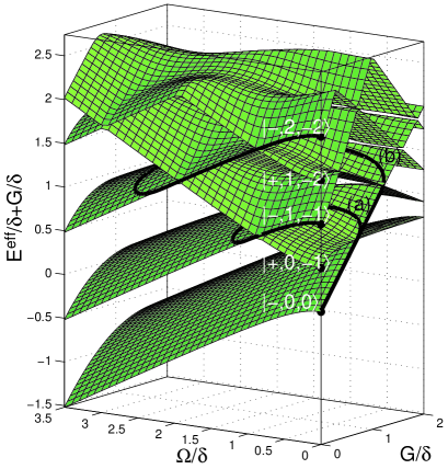
Figure 2: First five eigenenergy surfaces (in units of $\delta$) of $H^{\text{eff}}$ as functions of $G$ and $\Omega$ for $\delta=2\Delta_{M}=-2\Delta_{C}$. The term $G$ has been added to $E^{\text{eff}}$ for clarity of display. The solid paths(a,b) correspond to adiabatic evolutions which start from $|-,0,0\rangle$ state and end at $|-,1,-1\rangle$ and $|-,2,-2\rangle$ respectively.

We consider the action of two smooth pulses, associated with the Rabi frequencies $G(t)$ and $\Omega(t)$, which act on the two-level atom with a time delay $\tau=d/v$. Figure 2 shows two examples of the adiabatic paths of different peak amplitudes of the Rabi frequencies and leading to two different photon transfers into the cavity field without changing the atomic population at the end of the interaction. Each of the two black paths (labelled (a) and (b)) corresponds to a sequence of two smooth pulses, shown in Fig. 3(a) and (c), of equal length $T_{int}$ and different peak Rabi frequencies $\Omega_{\text{max}},G_{\text{max}}$ , separated by a delay such that the cavity pulse interacts before the maser pulse.

For the path (a), the dynamics goes through the first intersection (on the $\Omega=0$ plane) between the first and the second surfaces, but not the second intersection between the second and the third surface. The crossing of the first intersection as $G$ increases with $\Omega=0$, brings the dressed system into the second eigenenergy surface. Turning on and increasing the amplitude $\Omega$ (while $G$ decreases) moves the path across this surface. When the maser field decreases, the curve crosses another intersection between the second and the third surface (with $G=0$) that brings the system to the third surface, on which the path (a) stays until the end of the pulse $\Omega$. The transfer state is finally connected to the state $|-,1,-1\rangle$: there is no final transfer of atomic population, but one $\omega_{M}$ photon has been absorbed from the maser field and one $\omega_{C}$ photon has been emitted into the cavity field at the end of the process. The path (b) allows the dynamics (on the $\Omega=0$ plane) to go through the second intersection, but not the third intersection. The next two intersections of the path (b) are located (on the plane $G=0$) between the third and the fourth and between the fourth and the fifth eigenenergy surfaces and the system is finally connected to the state $|-,2,-2\rangle$: there is again no final transfer of atomic population, but two $\omega_{M}$ photons have been absorbed from the maser field and two $\omega_{C}$ photons have been emitted into the cavity field at the end of the process. If the peak amplitudes are taken even larger such that $n$ conical intersections (dynamical resonances) are crossed when $G$ rises with $\Omega=0$ and then $n$ intersection are crossed when $\Omega$ decreases with $G=0$, the final state of the system will be $|-,n,-n\rangle$, i.e., the emission of $n~{}~{}\omega_{C}$ photons into the cavity field and the absorbtion of $n~{}~{}\omega_{M}$ photons from the maser field, with no final atomic population transfer.

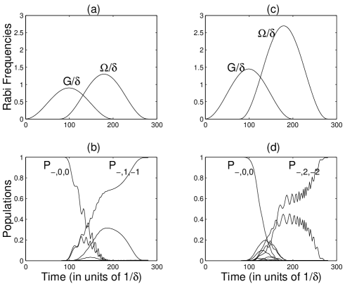
Figure 3: (a) and (c): Normalized Rabi frequencies with different values of amplitudes for one-photon and two-photon transfers as a function of time. (b) and (d): Time evolution of the populations for one and two-photon transfers.

The analysis of the eigenenergy surfaces allows one to determine adapted amplitudes of the Rabi frequencies which will permit to transfer $n$ photons into the cavity field in a robust way.

IV numerical simulation

The time evolution of the system for each family of the eigenenergy surfaces is given by the Schrödinger equation

$$i\frac{\partial}{\partial t}\Phi(t)=H^{\text{eff}}(t)\Phi(t)$$ (44)

The time dependence of the Rabi frequencies are delayed Gaussians of the form (II). Figures 3(a),(c) show the profile of the Rabi frequencies as functions of time for one-photon and two-photon transfer with an interaction time (full width at half maximum) $T_{int}=66/\delta$ and a time delay $\tau=57/\delta$. The adapted amplitudes of the Rabi frequencies for $n$-photon ($n$=1,2) transfer correspond to the paths (a) and (b) in Fig. 2. The condition for global adiabaticity $|\Delta_{M,C}|T_{int}=\frac{\delta}{2}T_{int}=33\gg 1$ is well satisfied. Figures 3(b,d) present the time evolution of populations calculated numerically by solving (44). The atom-maser-cavity system in the initial state $|-,0,0\rangle$ with the suitable forms of Rabi frequencies (Figs. 3(a,c)) evolves to the finale states $|-,1,-1\rangle$ and $|-,2,-2\rangle$ respectively with probabilities of $P_{-,1,-1}=|\langle-,1,-1|\Phi(t_{f})\rangle|^{2}=0.99$ and $P_{-,2,-2}=|\langle-,2,-2|\Phi(t_{f})\rangle|^{2}=0.98$.

Fig. 4 displays the contour plot of the final population as a function of the normalized Rabi frequencies for one and two-photon transfers. The white regions represent the adapted values of the Rabi frequencies for which the final probability of one and two-photon transfers are maximal. This figure shows that the bichromatic adiabatic passage is more robust with respect to the maser Rabi frequency than with respect to the cavity one. The reason comes back to the special structure of the dressed eigenenergy surfaces in Fig. 2. We can see that on the $G=0$ plane, between the first surface and the second one there isn’t any intersection and between the $n$th surface and its neighboring surfaces there are $(n-1)$ intersections, i.e. after the ($n-1$)th intersection there are no others. On the other hand on the $\Omega=0$ plane, as the value of $G$ increases, the distance between neighboring intersections decreases. In general, as the distance of conical intersections between neighboring surfaces decreases, the robustness of the adiabatic passage is also decreased.

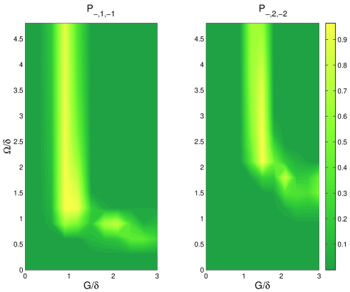
Figure 4: Contour plot of the populations $P_{-,1,-1}$ and $P_{-,2,-2}$ for one-photon and two-photon transfers as a function of normalized Rabi frequencies.

V discussions and conclusions

Using the topological properties of dressed eigenenergy surfaces of the effective Hamiltonian of the atom-maser-cavity system, we have determined adiabatic paths to transfer $n$ photons from the maser field into the cavity field to generate a $n$-photon Fock state. The realization of parameters satisfying the conditions of the proposed scheme appears feasible with progressive improvements to experiments with high-Q microwave cavities. In this analysis we have assumed that the interaction time between the two-state atom and the fields is short compared to the cavity lifetime $T_{\text{cav}}$ and the atom’s excited state lifetime $T_{\text{at}}$, i.e. $T_{\text{int}}\ll T_{\text{cav}},T_{\text{at}}$, which are essential for an experimental setup and avoiding decoherence effects. In the microwave domain, the radiative lifetime of circular Rydberg states – of the order of $T_{\text{at}}=30$ms – are much longer than those for noncircular Rydberg states. The typical value of the cavity lifetime is of the order of $T_{\text{cav}}=1$ ms (corresponding to $Q=3\times 10^{8}$) and the upper limit of interaction time is $T_{\text{int}}=100$ $\mu$s (atom with a velocity of 100 m/s with the cavity mode waist of $W_{C}=6$ mm) Raimond et al. (2001).

The condition of global adiabaticity $G_{\text{max}}~{}T_{\text{int}}\gg 1$ for the typical value of $G_{\text{max}}\approx 0.15$ MHz Raimond et al. (2001) is well satisfied $(G_{\text{max}}~{}T_{\text{int}}\approx 15$). Analysis for additional conditions to go diabatically through conical intersections can be found in Yatsenko et al. (2002).