Diffraction of ultra-cold fermions by quantized light fields: Standing versus traveling waves

Abstract

We study the diffraction of quantum degenerate fermionic atoms off of quantized light fields in an optical cavity. We compare the case of a linear cavity with standing wave modes to that of a ring cavity with two counter-propagating traveling wave modes. It is found that the dynamics of the atoms strongly depends on the quantization procedure for the cavity field. For standing waves, no correlations develop between the cavity field and the atoms. Consequently, standing wave Fock states yield the same results as a classical standing wave field while coherent states give rise to a collapse and revivals in the scattering of the atoms. In contrast, for traveling waves the scattering results in quantum entanglement of the radiation field and the atoms. This leads to a collapse and revival of the scattering probability even for Fock states. The Pauli Exclusion Principle manifests itself as an additional dephasing of the scattering probability.

I Introduction

The past few decades have witnessed considerable progress in the cooling of atomic vapors to extremely low temperatures, culminating in the achievement of Bose-Einstein condensation in dilute alkali gases Anderson et al. (1995); Bradley et al. (1995); Davis et al. (1995). More recently, quantum degenerate Fermi gases with temperatures as low as $0.01T_{F}$, where $T_{F}$ is the Fermi temperature, have been achieved by several groups Regal et al. (2004); Hadzibabic et al. (2003); Strecker et al. (2003). Throughout these developments the interaction of light with atoms has been central to the cooling, trapping, and imaging of atoms, as well as in the coherent manipulation of their center-of-mass motion. For example, the Bragg scattering of atomic matter waves by off-resonant optical fields can be used to create linear atom optical elements for use in atom interferometers Burgbacher and Audretsch (1999), and the interaction of atomic condensates with light has led to the realization of matter-wave superradiance Inouye et al. (1999a) and of matter-wave parametric amplifiers Kozuma et al. (1999); Inouye et al. (1999b); Law and Bigelow (1998). In another application, the ability of optical fields to create custom trapping potentials has permitted the study of condensed matter problems such as e.g. the Mott-Insulator transition Jaksch et al. (1998); Greiner et al. (2002a, b). Although all experiments to date have involved classical optical fields, there is considerable interest in carrying out future work in high-Q optical cavities, where the quantum nature of the electromagnetic field becomes important. Theoretical work along these lines has so far been restricted to the case of bosonic atoms, see e.g. Ref. Moore et al. (1999), while the diffraction of fermions by an optical field was discussed in Ref. Lenz et al. (1993), but in an analysis restricted to the case of classical fields. In this paper we extend this work to discuss the diffraction of quantum-degenerate fermionic matter-wave fields by quantized light fields.

We consider a zero-temperature beam of fermionic two-level atoms traversing an optical cavity supporting an off-resonant standing wave light field of momentum $q$. The atoms undergo virtual transitions to their excited electronic state, resulting in a center-of-mass momentum recoil of $2q$ . Alternatively, one can view this process as diffraction of the atoms off of the intensity grating formed by the cavity field.

The normal modes in terms of which the electromagnetic field is quantized are determined by the boundary conditions of the cavity. In a linear cavity with perfectly reflecting mirrors we have standing wave mode functions. In a ring cavity, the light field has to fulfill periodic boundary conditions and this results in running-wave mode functions. Two counter-propagating traveling wave modes of equal frequency can be superposed to yield a stationary standing wave field.

Under most circumstances it is a question of mathematical convenience which mode functions are used for the description of the field. Physically, however, the two cases are not the same and for fields containing only a few photons, the two quantization procedures yield different results. In particular, the difference in atomic scattering produced in these two situations has been discussed for single atoms diffracted by a coherent light field Shore et al. (1991). It was shown to depend critically on the quantization procedure. This difference can be understood in terms of which-way information for the scattering process. For standing wave modes, the state of the light field contains no information about the momentum transfer to the atom. More specifically, the number of photons is a constant of motion and as a result the equations of motion for the atomic center of mass decouple from that of the light field. In the case of two counter-propagating traveling wave modes however, the number of photons in each mode does change and the change in the number of quanta is a direct measure of the momentum transfer to the atoms. In this paper we extend those results to compare the diffraction of a quantum-degenerate Fermi gas by these fields, both in the Raman-Nath and Bragg regimes.

In the Raman-Nath regime, which is characteristic of situations where the kinetic energy of the atoms can be neglected, the individual atomic dynamics for a standing wave light field are formally identical to the case of a classical light field Meystre and III (1999). The atoms scatter into successive diffraction orders separated by twice the photon momentum $q$, up to the point where energy-momentum conservation becomes important and the Raman-Nath approximation ceases to hold. The formal equivalence of the scattering off of a standing wave field to the scattering off of a classical light field is due to the fact that the equations of motion for the atoms effectively decouple both from each other and from the light field. This must be contrasted to the case of running waves, where the number operators for the two modes are not constants of motion. This leads to an infinite hierarchy of coupled equations for the atomic and optical field operators, with higher-order correlation functions playing a crucial role in the dynamics of first-order atomic correlation functions. It is then necessary to introduce some approximate truncation scheme, a procedure that we discuss in detail and compare with exact numerical results for small atom numbers.

In the Bragg regime, energy-momentum conservation reduces the single-atom diffraction problem to a two-mode situation, the atoms undergoing Bragg oscillations between their initial momentum states, $p_{i}$, and final momentum state $p_{f}=p_{i}+2q$. The character of these oscillations is the result of three separate and independent effects which correspond to whether one uses standing wave or traveling wave modes, whether the cavity field is in a Fock state or in a coherent state, and the momentum spread of the incident atomic beam.

This paper is organized as follows: After formulating the specific model used in our analysis in section II we discuss the case of traveling-wave light quantization in section III. We develop approximate equations for first and second-order correlation function appropriate for the Raman-Nath regime, and a Bloch vector picture useful to discuss Bragg diffraction. Specifically, that picture yields a semiclassical model that provides some intuitive understanding of the atomic dynamics. The case of standing-wave quantization is discussed in Section IV. Section V gives a summary and conclusion.

II Model

We consider an ultracold beam of identical two-level fermionic atoms propagating across a high-$Q$ optical cavity, see Fig. 1. Their initial momentum distribution is a Fermi sea at $T=0$, but shifted in momentum space by the mean momentum ${\bf{p}}$ and with Fermi momentum $k_{F}$ assumed to be much less than $q$, the photon momentum. This is a realistic approximation, since for a degenerate Fermi gas of density $n\approx 10^{17}\text{m}^{-3}$ the Fermi momentum is $k_{F}\approx 10^{6}\text{m}^{-1}$ while for a photon of wavelength $\lambda=500\text{nm}$ one has a momentum of $q\approx 10^{7}\text{m}^{-1}$. In the following we neglect atomic collisions – a good approximation at low temperatures, since the $s$-wave scattering length is zero for identical fermions – as well as cavity losses. We also assume that the optical frequency $\omega$ is sufficiently detuned from the atomic transition frequency $\omega_{0}$ that the upper electronic level can be adiabatically eliminated. Finally, we consider a situation where that atomic momentum $mv_{\perp}$ transverse to the cavity field is large enough so that it can be treated classically. Time, $t$, can then be parameterized in terms of the transverse distance $x$ by $t=x/v_{\perp}$.

Figure 1: (a) Schematic of a scattering of an atom of initial momentum $p$ via two photon transitions with photons of momenta $q$ and $-q$. (b) Initial momentum distribution $N(p)$ of the atoms for scattering in the Raman-Nath regime and (c) for the Bragg regime.

III Running waves

For running-wave quantization, the Hamiltonian describing our system is $(\hbar=1)$

$$H_{r} = \sum_{k}E_{k}c^{\dagger}_{k}c_{k}+\omega(a_{q}^{\dagger}a_{q}+a_{-q}^{\dagger}a_{-q}+1)$$ (1)

$$+ \left(ga_{q}^{\dagger}a_{-q}\sum_{k}c^{\dagger}_{k-q}c_{k+q}+h.c.\right),$$

where, $c_{k}$ and $c_{k}^{\dagger}$ are the annihilation and creation operators for a fermionic atom of momentum $k$, $a_{q}$ and $a_{q}^{\dagger}$ are the annihilation and creation operators for a photon of momentum $q$, $E_{k}=k^{2}/2M$ is the kinetic energy of an atom of momentum $k$, $g=\Omega_{R}^{2}/\Delta$ is the coupling energy of the atoms and the light field, $\Omega_{R}$ is the vacuum Rabi frequency, and $\Delta=\omega-\omega_{0}$ is the atom-light detuning.

The initial state of the atoms-field system is

$$|\psi(0)\rangle_{\rm rw}=|\phi_{q}\rangle|\phi_{-q}\rangle\prod_{|k|<k_{F}}c_{k}^{\dagger}|0\rangle.$$ (2)

where the field states $|\phi_{\pm q}\rangle$ are taken to be either Fock states $|N_{\pm q}\rangle$ or coherent states $|\alpha_{\pm q}\rangle$.

III.1 Raman-Nath regime

The Raman-Nath regime of atomic diffraction is characteristic of situations where the kinetic energy of the atoms plays a negligible role in comparison with the interaction energy, i.e. $E_{2q}\ll g\sqrt{N_{q}N_{-q}}$, where the recoil energy $E_{2q}=2q^{2}/M$ is a measure for the typical kinetic energies involved. In practice, this amounts to assuming that the atoms have an infinite mass, and as such, neglects the effects of the quadratic dispersion relation of the atoms.

The most straightforward way to solve this problem proceeds by integrating the Schrödinger equation corresponding to Hamiltonian (1) for the initial conditions (2), From which we can obtain the probability

$$P_{p}(t)=\langle\psi(t)|c_{p}^{\dagger}c_{p}|\psi(t)\rangle.$$ (3)

for an atom being scattered to a state of momentum $p$. However, the dimension of the Hilbert space grows exponentially as ${\rm Dim}_{\rm Raman-Nath}=(2n_{d}+1)^{N_{a}}(N_{p}+1)$ where $n_{d}$ is the number of diffraction orders considered, $N_{a}$ is the number of atoms, and $N_{p}$ the total number of photons. Hence, a direct integration of the Schrödinger equation is only possible for rather small atom and photon numbers.

Figure 2(a) shows the result of an exact solution of the Schrödinger equation for $N_{a}=2$ and the light field in a Fock state with three photons per mode initially. In this example, the recoil energy is $E_{2q}=g$ and the initial momentum of the atoms is $p_{i}=\pm 0.1q$. Such a high recoil energy was chosen to limit the number of diffraction orders that are significantly populated before energy-momentum conservation inhibits further diffraction, i.e. before exiting the Raman-Nath regime.

The resulting dynamics resembles qualitatively the single-atom case, see e.g. Meystre and III (1999). For short times the probability for finding an atom in the $m$th order mode is well described by $\sim J_{m}^{2}(2gt)$ where $J_{m}$ is the $m$-th Bessel function. For longer interaction times, higher scattering orders are suppressed due to energy-momentum conservation, as expected. We note that since the difference in kinetic energies of the two atoms is small compared to all other relevant energies, we do not observe any effect of “inhomogeneous broadening.”

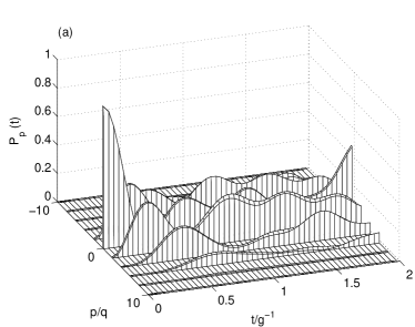
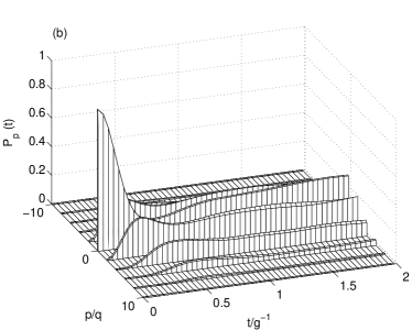
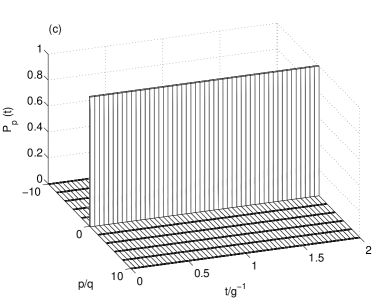
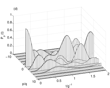
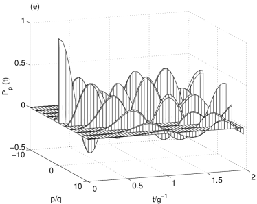
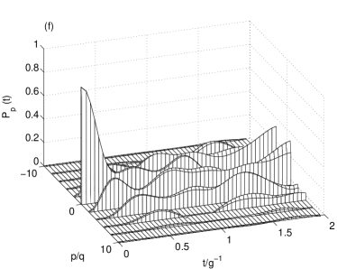
Figure 2: Scattering probability $P_{p}(t)$ for two atoms scattering off of a running-wave light field in the Raman-Nath regime. Figures (a,c,e) are for a Fock state of the light field and figures (b,d,f) for a coherent state. Figures (a,b) show the exact solution of the Schrödinger equation, figures (c,d) for the first-order equations and figures (e,f) show the results for the second-order equations. In all the calculations the recoil energy is $E_{2q}=g$ and the Fermi momentum is $k_{F}=0.1$. Time is in units of $g^{-1}$ and momentum in units of the photon momentum $q$.

For comparison, the results for initial coherent states with mean photon numbers $\overline{N}_{q}=\overline{N}_{-q}=3$ are shown in Fig. 2(b), the atomic parameters being the same as before. We now observe a decay of the oscillations of the scattering probabilities after a time $t\sim(2\pi/g)(\overline{N}_{q}\overline{N}_{-q})^{-1/2}$, which corresponds to a complete dephasing of the contributions of the different photon numbers to the diffraction pattern.

In order to proceed past the few-atom problem, we now concentrate on single-particle properties, introducing a BBGKY-type truncation scheme to factorize higher-order correlation functions of the matter-wave field. From the Hamiltonian (1), the equations of motion for the atomic first order correlations $\langle c_{k_{1}}^{\dagger}c_{k_{2}}\rangle$ and $\langle a_{q_{1}}^{\dagger}a_{q_{2}}\rangle$,

$$i\frac{d}{dt}\langle c_{k_{1}}^{\dagger}c_{k_{2}}\rangle=(E_{k_{2}}-E_{k_{1}})\langle c_{k_{1}}^{\dagger}c_{k_{2}}\rangle+g\left\langle a_{-q}^{\dagger}a_{q}\left(c_{k_{1}}^{\dagger}c_{k_{2}-2q}-c_{k_{1}+2q}^{\dagger}c_{k_{2}}\right)\right\rangle+g\left\langle a_{q}^{\dagger}a_{-q}\left(c_{k_{1}}^{\dagger}c_{k_{2}+2q}-c_{k_{1}-2q}^{\dagger}c_{k_{2}}\right)\right\rangle,$$ (4)

$$i\frac{d}{dt}\langle a_{q_{1}}^{\dagger}a_{q_{2}}\rangle=g\sum_{k}\left\langle\delta_{q_{2},q}a_{q_{1}}^{\dagger}a_{-q}c_{k-q}^{\dagger}c_{k+q}+\delta_{q_{2},-q}a_{q_{1}}^{\dagger}a_{q}c_{k+q}^{\dagger}c_{k-q}+\delta_{q_{1},-q}a_{q}^{\dagger}a_{q_{2}}c_{k-q}^{\dagger}c_{k+q}+\delta_{q_{1},q}a_{-q}^{\dagger}a_{q_{2}}c_{k+q}^{\dagger}c_{k-q}\right\rangle,$$ (5)

where the $\delta$’s are Kronecker-deltas.

The simplest factorization scheme consists in merely factorizing second-order correlation functions of the type $\langle a_{q_{1}}^{\dagger}a_{q_{2}}c_{k_{1}}^{\dagger}c_{k_{2}}\rangle$ that appear on the right-hand side of these equations into products of first-order correlation functions, for instance, $\langle a_{q_{1}}^{\dagger}a_{q_{2}}c_{k_{1}}^{\dagger}c_{k_{2}}\rangle\approx\langle a_{q_{1}}^{\dagger}a_{q_{2}}\rangle\langle c_{k_{1}}^{\dagger}c_{k_{2}}\rangle$ . In doing so we neglect correlations that may build up between the atoms and the light field as well as higher-order correlations of both the atoms and the light field. This corresponds to a truncation of the BBGKY-type hierarchy of the equations of motion for the higher-order moments of the particle-hole operators after the first order, see e.g. Huang (1987). This reduces the infinite hierarchy of equations (4-5) to a closed set of $c$-number equations that grows only quadratically with the number of momentum states that have to be taken into account.

The result of the numerical integration of these equations of motion, using the same parameters as previously for ease of comparison, is shown in Fig.2(c,d) for the cases of a Fock state and a coherent state of the field, respectively.

An obvious weakness of the simple truncation scheme is that it predicts the absence of scattering for the case of Fock states, in stark contrast to the exact solution. This follows from the absence of initial coherence in either the light field or the atoms, leading to the scattering term in (4) being identically zero. Stated differently, the reason for the absence of diffraction is that the phase of a Fock state is completely undetermined, hence there is no established relative phase between the two counter-propagating fields, and no light intensity grating. Since in this factorization scheme the atom is effectively assumed to probe only first-order moments of the light field, that is, its intensity pattern, diffraction is absent at this level of approximation.

The situation is different for a coherent state light field. In this case, there is a well-established phase relationship between the two modes. This results in an intensity grating from which the atoms can be diffracted. As time goes on, this results in the generation of atomic coherence, $\langle c_{k_{1}}^{\dagger}c_{k_{2}}\rangle\neq 0$, and the resulting density grating formed by the atoms acts back on the light field. In some loose sense, the lowest order factorization scheme consists in treating the system classically since it neglects all quantum fluctuations in the atomic and optical fields. It is not surprising that this approach should fail for a very non-classical field state such as a Fock state, and be much better for a quasi-classical field. Note however that while for short enough times the scattering closely resembles the exact results, this is no longer the case for long times, a consequence of the build-up of quantum correlations between the optical and matter-wave fields. Even after one oscillation differences arise.

We note that for our specific initial conditions, the fully factorized equations for the light field can be trivially integrated, showing that the first-order moments of the light field are constants of motion. Inserting these constants in the atomic equations of motion shows that at this level, the scattering becomes formally equivalent to the scattering of atoms by a classical standing wave light field with intensity $g\langle a_{q}^{\dagger}a_{-q}\rangle$. This is further discussed in the following section.

The equations of motion (4-5), suggest that an improved factorization scheme would retain the lowest order correlations between light field and atoms. In order to do so, we supplement the equations of motion for $\langle c_{k_{1}}^{\dagger}c_{k_{2}}\rangle$ and $\langle a_{q_{1}}^{\dagger}a_{q_{2}}\rangle$ by equations of motion for the cross-correlations $\langle a_{q_{1}}^{\dagger}a_{q_{2}}c_{k_{1}}^{\dagger}c_{k_{2}}\rangle$ and the second order correlations of the lightfield and the atoms. This should remedy the major flaw of the first-order calculation, namely its inability to predict atomic scattering for a light field in a Fock state.

The equations for the lowest-order atom-field correlation functions involve third-order correlations of the form $\langle a_{q_{1}}^{\dagger}a_{q_{2}}a_{q_{3}}^{\dagger}a_{q_{4}}c_{k_{1}}^{\dagger}c_{k_{2}}\rangle$ and $\langle a_{q_{1}}^{\dagger}a_{q_{2}}c_{k_{1}}^{\dagger}c_{k_{2}}c_{k_{3}}^{\dagger}c_{k_{4}}\rangle$. We truncate the resulting hierarchy of equations of motion by introducing the factorization scheme

$$\langle a_{q_{1}}^{\dagger}a_{q_{2}}a_{q_{3}}^{\dagger}a_{q_{4}}c_{k_{1}}^{\dagger}c_{k_{2}}\rangle\simeq\langle a_{q_{1}}^{\dagger}a_{q_{2}}\rangle\langle a_{q_{3}}^{\dagger}a_{q_{4}}c_{k_{1}}^{\dagger}c_{k_{2}}\rangle+\langle a_{q_{1}}^{\dagger}a_{q_{2}}a_{q_{3}}^{\dagger}a_{q_{4}}\rangle\langle c_{k_{1}}^{\dagger}c_{k_{2}}\rangle+\langle a_{q_{1}}^{\dagger}a_{q_{2}}c_{k_{1}}^{\dagger}c_{k_{2}}\rangle\langle a_{q_{3}}^{\dagger}a_{q_{4}}\rangle-2\langle a_{q_{1}}^{\dagger}a_{q_{2}}\rangle\langle a_{q_{3}}^{\dagger}a_{q_{4}}\rangle\langle c_{k_{1}}^{\dagger}c_{k_{2}}\rangle$$ (6)

and similarly for $\langle a_{q_{1}}^{\dagger}a_{q_{2}}c_{k_{1}}^{\dagger}c_{k_{2}}c_{k_{3}}^{\dagger}c_{k_{4}}\rangle$ with $a_{q}$’s replaced by $c_{k}$’s and vice versa Anglin and Vardi (2001). The last term of this equation accounts for the case where all first-order correlation functions are uncorrelated.

We estimate the accuracy of the factorization scheme by calculating $\langle a_{q_{1}}^{\dagger}a_{q_{2}}a_{q_{3}}^{\dagger}a_{q_{4}}c_{k_{1}}^{\dagger}c_{k_{2}}\rangle$ and $\langle a_{q_{1}}^{\dagger}a_{q_{2}}c_{k_{1}}^{\dagger}c_{k_{2}}c_{k_{3}}^{\dagger}c_{k_{4}}\rangle$ as well as their respective factorized values, Eq. (6) using the exact solution of the Schrödinger equation. As an example Fig. 3 shows the results for $\langle a_{-q}^{\dagger}a_{q}a_{q}^{\dagger}a_{-q}c_{k_{F}}^{\dagger}c_{k_{F}}\rangle$ and Fig. 4 shows the results for $\langle a_{q}^{\dagger}a_{q}c_{k_{F}}^{\dagger}c_{k_{F}}c_{k_{F}}^{\dagger}c_{k_{F}}\rangle$ for the parameters of Fig. 2. This shows that the factorization scheme reproduces at least qualitatively the main features of the third-order correlation functions for both coherent states and Fock states.

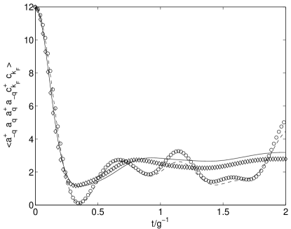
Figure 3: Expectation value of $a_{-q}^{\dagger}a_{q}a_{q}^{\dagger}a_{-q}c_{k_{F}}^{\dagger}c_{k_{F}}$ as calculated from the numerical solution of the Schrödinger equation for a Fock state and for a coherent state of the light field with the same parameters that were used in Fig. 2. $\circ$ and $\diamond$ show the exact unfactorized value for Fock state and coherent state respectively; the broken line ($-\hskip 2.84544pt-$) and the solid line (—) show the corresponding values for the Fock state and coherent state as obtained with the factorization scheme (6).

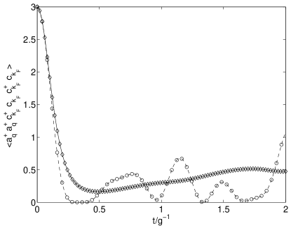
Figure 4: Expectation value of $a_{q}^{\dagger}a_{q}c_{k_{F}}^{\dagger}c_{k_{F}}c_{k_{F}}^{\dagger}c_{k_{F}}$ as calculated from the numerical solution of the Schrödinger equation for a Fock state and for a coherent state of the light field with the same parameters that were used above. $\circ$ and $\diamond$ show the exact unfactorized value for Fock state and coherent state respectively. The broken line ($-\hskip 2.84544pt-$) and the solid line (—) show the values obtained from the factorization scheme (6) for the two cases.

Despite its apparent success, we must keep in mind that this factorization scheme suffers from two major flaws. First, the small deviations of the factorized values from the exact values will accumulate in the course of time, leading to increasing discrepancies between the approximate and exact results. More critical perhaps, this scheme violates important relations that the exact operators have to obey. For example, $a_{q}^{\dagger}a_{q}c_{k_{F}}^{\dagger}c_{k_{F}}c_{k_{F}}^{\dagger}c_{k_{F}}$ is a positive self-adjoint operator, with positive and real expectation values, but the factorized approximation can take on negative values. These flaws eventually result in non-physical behavior such as illustrated in Fig. 2(e,f) where the probabilities $\langle c_{k}^{\dagger}c_{k}\rangle$ take on negative values. We have not found a factorization scheme that avoids non-physical behavior of that kind at all times, and conjecture that the factorization of higher-order moments in lower-order moments necessarily leads to such inconsistencies.

The results of the factorization scheme (6) are shown in Fig. 2(e) for a Fock state and in Fig. 2(f) for a coherent state of the light field. While a Fock state now leads to atomic diffraction, as should be the case, it is characterized by non-physical negative probabilities already for short times. This is clear evidence that higher order correlations play an essential role. This is in contrast with the situation for a coherent state, where we achieve good agreement with the exact results for times up to $\sim(2\pi/g)(\overline{N}_{q}\overline{N}_{-q})^{-1/2}$, indicating that the first and second-order correlations are the most important.

A quantitative measure of the degree of entanglement between the atoms and the light field is given by the second-order cross-correlation

$$\chi(t)=\sum_{k}\left(\langle a_{q}^{\dagger}a_{-q}c_{k-q}^{\dagger}c_{k+q}\rangle-\langle a_{q}^{\dagger}a_{-q}\rangle\langle c_{k-q}^{\dagger}c_{k+q}\rangle\right),$$ (7)

which is equal to zero in the absence of entanglement. Figure 5 shows $\chi(t)$ for both a Fock state and for a coherent state light field, for the parameters of Fig.2. Because the light field and atoms are initially uncorrelated we have $\chi(t=0)=0$ but cross-correlations then build up to become of the order of $(\overline{N}_{q}\overline{N}_{-q})^{1/2}N_{a}$. The figure also shows the result of the factorization ansatz (6), showing the good agreement with the exact result for short enough times.

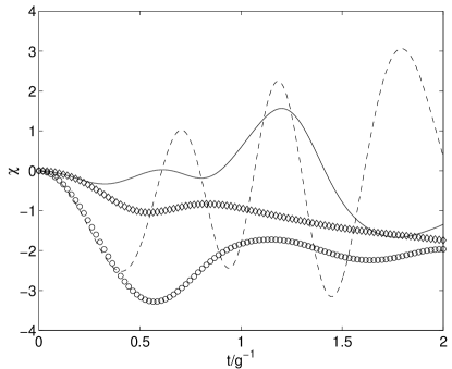
Figure 5: Cross-correlation $\chi(t)$ between light field and atoms in the Raman-Nath regime as obtained from the exact solution of the Schrödinger equation for a Fock state ($\circ$) and a coherent state of the light field ($\diamond$). Also shown are the values obtained from the factorization scheme (6) ($-\hskip 2.84544pt-$) for a Fock-state light field and (—) for a coherent state. Same parameters as in Fig. 2.

III.2 Bragg regime

In the Bragg regime, energy-momentum conservation restricts the scattering of the atoms to two diffraction orders, an initial mode of transverse momentum $p_{i}\approx-q$ and a final mode of momentum $p_{f}=p_{i}+2q\approx q$. Classically, the atoms are known to undergo Pendellösung oscillations between these two modes. As such, the atoms can be thought of as two-state systems that are conveniently described in terms of pseudo-spin operators

$$S_{k}^{z} = \frac{1}{2}\left(c_{k+q}^{\dagger}c_{k+q}-c_{k-q}^{\dagger}c_{k-q}\right)$$

$$S_{k}^{+} = (S_{k}^{-})^{\dagger}=c_{k+q}^{\dagger}c_{k-q}.$$ (8)

Introducing further the Schwinger representation of the light field by means of

$$J^{z} = \frac{1}{2}\left(a_{q}^{\dagger}a_{q}-a_{-q}^{\dagger}a_{-q}\right)\ ,$$

$$J^{+} = (J^{-})^{\dagger}=a_{q}^{\dagger}a_{-q},$$ (9)

the Hamiltonian of the atoms-field system simplifies to

$$H=\sum_{k\in[-k_{F},k_{F}]}\left(\delta\omega_{k}S_{k}^{z}+gJ^{+}S_{k}^{-}+gJ^{-}S_{k}^{+}\right).$$ (10)

In this representation, the eigenvalues $m$ of $J^{z}$ correspond to the photon number difference $m=(1/2)(N_{q}-N_{-q})$ between the two counter-propagating modes and the eigenvalues $j(j+1)$ of $J^{2}={J^{z}}^{2}+1/2(J^{+}J^{-}+J^{-}J^{+})$ correspond to the total number of photons, $j=1/2(N_{q}+N_{-q})$. Finally, $\delta\omega_{k}=E_{k+q}-E_{k-q}=2kq/M$ is the frequency mismatch between the two momentum states accessible to the atom with initial momentum $k-q$.

When compared to the Raman-Nath case, the dimension of the Hilbert-space is now reduced to ${\rm Dim}_{\rm Bragg}=(N_{p}+1)2^{N_{a}}$, which allows us to consider larger atomic and photon numbers. The initial state of the atoms is now a $T=0$ Fermi sea shifted by $-q$ in momentum. In the following, we evaluate the total number of atoms diffracted to states of momentum near $+q$,

$$N_{sc}(t)=\sum_{k\in[-k_{F},k_{F}]}P_{k+q}(t).$$ (11)

for a light field initially in a Fock state and in a coherent state.

III.2.1 Fock state

Figure 6(a) shows $P_{p_{f}}(t)$ for a Fock state with $N_{q}=N_{-q}=6$ photons and five atoms, with a recoil energy $E_{2q}=50g$ and the Fermi momentum is $k_{F}=0.1q$. Figure 7(a) show $N_{sc}(t)$ for the same parameters.

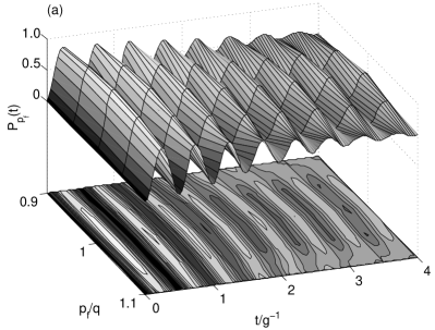
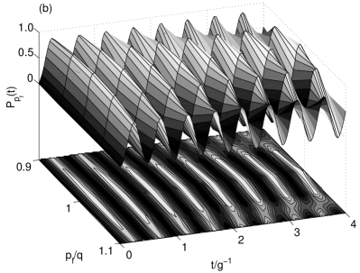
Figure 6: Scattering probability $P_{p_{f}}(t)$ for five fermions scattering off of a running-wave light field (a) and a standing-wave light field (b) in the Bragg regime. In both cases the light field is in a Fock state with $N_{q}=N_{-q}=6$ and $N=12$ respectively, $E_{2q}=50g$ and $k_{F}=0.1q$. Time in units of $g^{-1}$ and momentum in units of $q$.

For short times the atoms undergo Pendellösung oscillations between initial and final momentum states, with an amplitude that decreases as the atomic momentum is further detuned from the Bragg resonance condition. For longer times the oscillations of the individual atoms dephase, as expected from their different kinetic energies. However, the dephasing is not as strong as would be the case for a system of independent particles, such as in the standing-wave case discussed later on, a clear manifestation of the collective nature of the system.

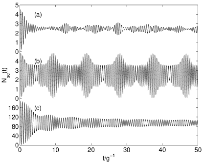
Figure 7: Mean number of scattered atoms, $N_{sc}=\sum P_{p_{f}}$ for Fock states of the light field and for different recoil energies.(a) Running wave light field with $N_{q}=N_{-q}=6$ photons in each of the two modes with recoil energy $E_{2q}=50g$. (b) Same light field as in (a) but without dephasing for the atoms, $E_{2q}=0$. (c) Standing wave light field with $N=6$ photons with recoil energy $E_{2q}=50g$ for 200 atoms. Time in units of $g^{-1}$.

In addition, the individual atomic oscillations undergo a decay that is intrinsically linked to the quantum correlations that build up between the light field and the atoms and is present even if we neglect dephasing (i.e. $k_{F}=0$), as shown in Fig.7(b). For zero dephasing, the amplitude of the oscillations eventually revives to its initial value. (The fact that the collapse of the oscillations and their subsequent revival resemble a beat phenomenon in the figure is an artifact from the comparatively small number of atoms and photons.) Combined with the inhomogeneous dephasing due to the width of the Fermi sea, this decay results in the total oscillation amplitude $N_{sc}(t)$ shown in Fig.7(a).

We can gain a qualitative understanding of the collapse and revival from an analysis of the matrix elements of the operators $J^{+}$ and $J^{-}$, which give an estimate of the transition frequencies for the atoms from $p_{i}$ to $p_{f}$: although for an initial Fock state the system starts in a state of definite $m$, it evolves over time into a linear superposition of $m$ states. The matrix elements of $J^{+}$ and $J^{-}$ between different $m$-states yield different Rabi frequencies and hence Bragg oscillation periods. Eigenstates of $J^{z}$ with eigenvalues $m$ and $m+1$ are coupled by the matrix element

$$\langle j,m+1|J^{+}|j,m\rangle=\sqrt{(j+m+1)(j-m)}.$$ (12)

We can therefore estimate the collapse time, $T_{\rm decay}$, by calculating the difference between the fastest and the slowest of these frequencies, the collapse time being roughly the time after which this frequency difference has produced a phase difference of $2\pi$. Under the assumption that all $m$-states contribute equally to the dynamics we find

$$T_{\rm decay} = \frac{2\pi g^{-1}}{\langle j,1|J^{+}|j,0\rangle-\langle j,j|J^{+}|j,j-1\rangle}$$ (13)

$$= \frac{2\pi g^{-1}}{\sqrt{(j+1)j}-\sqrt{2j}}.$$

This estimate gives satisfactory agreement with the actual decay time for small $j$ (it is within $\sim 10\%$ of the numerical result for our parameters), but breaks down for large $j$. We attribute this to the fact that the assumption that all $m$ states are initially equally populated is unphysical for large $j$.

The revival time of the Pendellösung oscillations can be evaluated in a similar fashion: The revivals occur when the Rabi frequencies for neighboring $m$-states differ in phase by $2\pi$. This gives

$$T_{\rm revival} = \frac{2\pi g^{-1}}{\langle j,1|J^{+}|j,0\rangle-\langle j,2|J^{+}|j,1\rangle}$$ (14)

$$= \frac{2\pi g^{-1}}{\sqrt{(j+1)j}-\sqrt{(j+2)(j-1)}},$$

which goes to infinity when $j\rightarrow\infty$. Note that this estimate is not limited to small $j$ values since it does not rest on the assumption of equal populations of all $m$ states.

The collapse and revival times can be evaluated more quantitatively from the spectrum of the Hamiltonian, as illustrated in Fig. 8. While the eigenfrequencies cover the whole spectrum rather densely, the initial state of the system is well described as a superposition of just a few groups of eigenstates, and hence only a few narrow bands of frequencies, which turn out to be almost equally spaced, significantly determine the atomic dynamics.

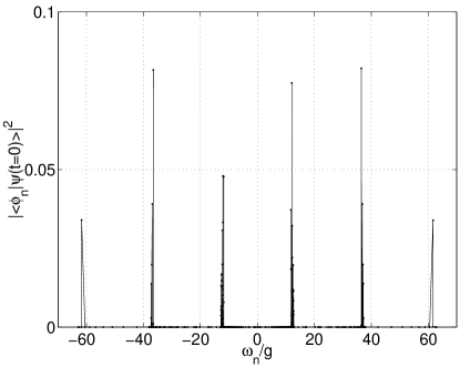
Figure 8: Projection of the initial conditions onto the spectrum of the Hamiltonian(10) for $N_{q}=N_{-q}=6$ photons, five atoms, a recoil energy of $E_{2q}=50g$ and a Fermi momentum of $k_{F}=0.1q$. Eigenfrequencies in units of $g$.

If these frequency bands were exactly evenly spaced the Pendellösung oscillations would be perfectly periodic. The variations in spacing and the widths of the various frequency bands lead to the more complicated dynamics.

The width of the frequency bands, which can be traced back to the usual dephasing of the atoms due to their spread in kinetic energies, gives the ordinary decay of the density oscillations, while the variation in separations between bands is a measure of the inverse revival time. Figure 9 shows this separation, obtained numerically for several photon numbers with and without dephasing. For comparison we also give the inverse revival time as determined from the matrix elements of $J^{+}$ as well as by a direct inspection of $N_{sc}(t)$. While the agreement between the revival times determined from the spectrum of the Hamiltonian and from $N_{sc}(t)$ is good for all photon numbers, the agreement with the estimate based on the matrix elements of $J^{+}$ improves for large photon numbers.

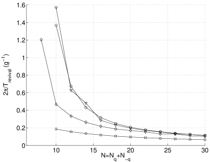
Figure 9: Inverse revival time $2\pi/T_{\rm revival}$ of the oscillations as determined from the spectrum of the Hamiltonian as a function of the photon number for $E_{2q}=50g$ and $k_{F}=0.1q$($\Diamond$). For comparison we also show the results without dephasing, $k_{F}=0$ ($\circ$) and the values obtained from comparing matrix elements of $J^{+}$, i.e. $\sqrt{(j+1)j}-\sqrt{(j+2)(j-1)}$ ($\square$). The inverse revival times as determined directly from simulations for $N_{sc}(t)$ like the one shown in Fig. 7(b) for no dephasing are also given ($\triangledown$). Frequencies are in units of $g$.

III.2.2 Coherent state

The case of a coherent state is readily obtained by averaging the Fock state results over a Poissonian photon distribution. The results for $P_{p_{f}}(t)$ and $N_{sc}(t)$ are given in Figs. 10(a) and 11(a), respectively. The oscillations of the mean number of scattered atoms as well as the Pendellösung oscillations of the individual atoms decay in a time $\lesssim g^{-1}$. In addition to the effects discussed in the previous section, we now have an additional dephasing due to the photon statistics of the coherent states. These independent dephasing processes are normally associated with non-commensurate decay rates and revival times, hence there are no revivals in this case.

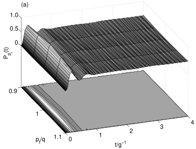
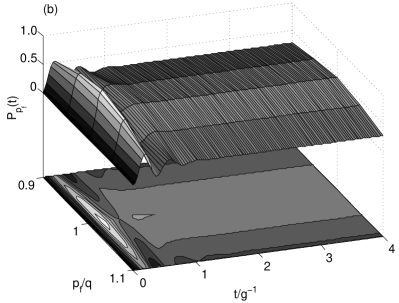
Figure 10: Scattering probability for five atoms scattering off (a) a running wave and (b) a standing wave in a coherent state. In both cases the recoil energy is $E_{2q}=50g$ and the Fermi momentum is $k_{F}=0.1q$. The mean number of photons is $\overline{N}_{q}=\overline{N}_{-q}=6$ in (a) and $\overline{N}=12$ in (b). Time is in units of $g^{-1}$ and momentum in units of $q$.

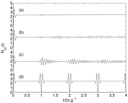
Figure 11: Mean number of scattered atoms $N_{sc}(t)$ in coherent state light fields. (a) Running-wave light field with mean photon numbers $\overline{N}_{q}=\overline{N}_{-q}=6$. The Fermi momentum is $k_{F}=0.1q$ and the recoil energy is $E_{2q}=50g$. (b) Light field as in (a), atoms without dephasing, i.e. $k_{F}=0$. (c) Standing-wave light field with mean photon number $\overline{N}=12$ and Fermi momentum $k_{F}=0.1q$ and recoil energy $E_{2q}=50g$. (d) Light field as in (c), but without dephasing for the atoms, $k_{F}=0$. Time in units of $2\pi g^{-1}$.

III.3 Bloch vector model

If we wish to consider greater atom numbers we can introduce a factorization scheme such as we used in the Raman-Nath regime. Here, the fact that the individual atoms are two-level systems in momentum space suggests that we use instead an approach analogous to the use of the Bloch vector in conventional quantum optics. We proceed by introducing the pseudo-spin vector ${\bf{S_{k}}}=S_{k}^{x}{\bf{\hat{x}}}+S_{k}^{y}{\bf{\hat{y}}}+S_{k}^{z}{\bf{\hat{z}}}$ where ${\bf{\hat{x}}}$, ${\bf{\hat{y}}}$, and ${\bf{\hat{z}}}$ are unit vectors along the $x$, $y$, and $z$ directions in the abstract Bloch vector space and

$$S_{k}^{x} = \frac{1}{2}(S_{k}^{+}+S_{k}^{-}),$$

$$S_{k}^{y} = \frac{1}{2i}(S_{k}^{+}-S_{k}^{-}),$$ (15)

(see Eq. (8)). The $S_{k}^{l},l=x,y,z$ obey the usual angular momentum commutation relations

$$\left[S_{k}^{l},S_{k^{\prime}}^{m}\right]=i\epsilon_{lmn}\delta_{k,k^{\prime}}S_{k}^{n},$$ (16)

where $\epsilon_{lmn}$ is the Levi-Civita symbol. Using these commutation relations we obtain the coupled equations of motion for the light field and atomic operators (10):

$$\frac{d{\bf J}}{dt} = g(S^{x}{\bf{\hat{x}}}+S^{y}{\bf{\hat{y}}})\times{\bf J},$$

$$\frac{d{\bf S}_{k}}{dt} = (\delta\omega_{k}{\bf{\hat{z}}}+g(J^{x}{\bf{\hat{x}}}+J^{y}{\bf{\hat{y}}}))\times{\bf{S}}_{k},$$ (17)

where we have introduced the total atomic spin operators

$$S^{l}=\sum_{k}S_{k}^{l}.$$

Equations (17) are exact within the two-state approximation of Bragg scattering. We can obtain a semiclassical picture by factorizing expectation values of products of atomic and field operators, e.g. $\langle S^{m}J^{n}\rangle=\langle S^{m}\rangle\langle J^{n}\rangle$.

For atoms with initial momenta centered around $-q$ we have $\langle S_{k}^{z}(0)\rangle=-1/2$, $\langle S_{k}^{x}(0)\rangle=\langle S_{k}^{y}(0)\rangle=0$ for all $k$, so that the individual atomic Bloch vectors point to the south pole. Likewise, for a field in a Fock state we have that $\langle J^{x}(0)\rangle=\langle J^{y}(0)\rangle=0$, so that ${\bf J}$ points along the ${\bf{\hat{z}}}$-axis, too. From the Bloch equations (17) it is then immediately apparent that there is no atomic scattering in the semiclassical description, consistently with the previous discussion.

For a coherent state, on the other hand, ${\bf J}$ is not parallel to the $z$-axis. For our choice of phase and for $\overline{N}_{q}=\overline{N}_{-q}$, it points instead along the $x$-direction. The phase relationship between the two counter-propagating coherent states leads to an intensity grating and the atoms will scatter off of it. Figure 12 shows the resulting scattering probability $P_{p_{f}}(t)$ obtained from this approximate model for five atoms and a light field initially in a coherent state with mean photon numbers $\overline{N}_{q}=\overline{N}_{-q}=6$.

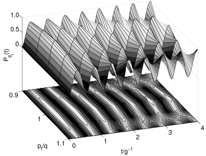
Figure 12: Scattering probability $P_{p_{f}}(t)$ for five atoms in a running-wave light field as calculated within the Bloch vector picture. The Fermi momentum is $k_{F}=0.1q$ and the recoil energy is $E_{2q}=50g$. Time in units of $g^{-1}$ and momentum in units of $q$.

The atomic Pendellösung oscillations do not decay as fast as in the full quantum description of Fig. 10(a). In the present picture, it can be attributed to the degradation of the intensity grating. The maximum oscillation amplitude occurs when ${\bf{J}}$ lies in the equatorial ${\bf{\hat{x}}}$-${\bf{\hat{y}}}$ plane, but the scattering of the atoms leads to a redistribution of the photons between the counter-propagating modes and a decrease in the optical fringe visibility.

IV Standing wave quantization

For a standing-wave quantization of the light field the Hamiltonian (1) is replaced by

$$H_{s}=\sum_{k}E_{k}c^{\dagger}_{k}c_{k}+\frac{g\hat{N}}{2}\sum_{k}c^{\dagger}_{k-q}c_{k+q}+H.C.$$ (18)

where $\hat{N}=a^{\dagger}a$, the number operator for the optical field mode, is clearly a constant of motion, and $a^{\dagger}$ and $a$ are bosonic creation and annihilation operators.

IV.1 Raman-Nath regime

From Eq. (18) we now have

$$i\frac{d}{dt}c_{k_{1}}^{\dagger}c_{k_{2}} = (E_{k_{2}}-E_{k_{1}})c_{k_{1}}^{\dagger}c_{k_{2}}$$

$$+\frac{g\hat{N}}{2}\left(c_{k_{1}}^{\dagger}c_{k_{2}-2q}+c_{k_{1}}^{\dagger}c_{k_{2}+2q}\right)$$

$$-\frac{g\hat{N}}{2}\left(c_{k_{1}+2q}^{\dagger}c_{k_{2}}+c_{k_{1}-2q}^{\dagger}c_{k_{2}}\right).$$

Since Eq. (18) does not couple states with different photon numbers, we can replace $\hat{N}$ by the corresponding eigenvalue $N$ for a particular number state, $|N\rangle$. We can then calculate the evolution of $\langle c_{k_{1}}^{\dagger}c_{k_{2}}\rangle$ for a general state of the field by averaging over the appropriate photon number distribution.

The equations for the first-order moments of the individual atoms are identical to those describing the scattering of a single atom by a classical light field, if one identifies $gN/2$ with the classical Rabi frequency. This follows from the absence of correlations between the light field and the atoms, together with the condition $q>k_{F}$, which implies the absence of Pauli blocking.

The scattering of a single atom by a classical field is a well-studied problem. An analytical solution is known in the Raman-Nath regime, see e.g. Rojo et al. (1999); Meystre and III (1999); Search et al. (2002). If the kinetic energy of the atoms is not negligible, on the other hand, one has to rely on a numerical solution.

Figure 13 shows the results for two atoms in a Fock state with N=6 photons. For short times the scattering clearly resembles the single-particle behavior, the probability of finding an atom in the $m$-th side mode being proportional to $J_{m}^{2}(gNt)$. Note that this result is identical to the approximate first-order calculation for the running-wave coherent state of section III.

The solution for a coherent state is obtained by averaging over a Poissonian photon number distribution. The result is shown in Fig. 14 for a mean photon number ${\bar{N}}=6$, which illustrates the dephasing due to the distribution of Rabi frequencies for such a state.

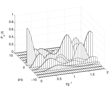
Figure 13: Scattering of two atoms off of a standing-wave light field in a Fock state with $N=6$ photons, the recoil energy is $E_{2q}=g$ and the Fermi momentum is $k_{F}=0.1q$. Time in units of $g^{-1}$ and momentum in units of photon momentum $q$.

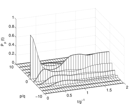
Figure 14: Scattering of two atoms off of a standing-wave light field in a coherent state. The mean number of photons is six, the recoil energy is $E_{2q}=g$ and the Fermi momentum is $k_{F}=0.1q$. Time in units of $g^{-1}$ and momentum in units of photon momentum $q$.

IV.2 Bragg regime

As previously discussed, the atoms can now be described in a two-state basis, leading to the effective Hamiltonian, see Eq. (10):

$$H=\sum_{k\in[-k_{F},k_{F}]}\left\{\delta\omega_{k}S_{k}^{z}+\frac{g\hat{N}}{2}(S_{k}^{-}+S_{k}^{+})\right\}.$$ (20)

Evidently, the Hamiltonian decomposes into independent single-particle Hamiltonians for the individual atoms, $H=\sum_{k}H_{k}$, so that the atomic equations of motion decouple and can be readily solved analytically. If the cavity is in a Fock state, the atoms undergo Pendellösung oscillations independently of each other, with a detuning given by $\delta\omega_{k}$. We then obtain

$$P_{p_{f}}(t)=\frac{(gN/2)^{2}}{\delta\omega_{k}^{2}+(gN/2)^{2}}\cdot\sin^{2}\left(\sqrt{\delta\omega_{k}^{2}+(gN/2)^{2}}t\right),$$ (21)

as illustrated in Fig. 6(b) for five atoms and the light field in a Fock state with $N=12$ photons. As expected, the frequency of the Pendellösung oscillations increases and their amplitude decreases with detuning, see Eq. (21). In contrast to the running-wave case, these oscillations remain perfectly sinusoidal for all times.

The oscillations in the mean number of scattered atoms $N_{sc}(t)$ is shown in Fig. 7(c) for an atom number of $200$. All other parameters are as before . Their decay due to the spread in detunings $\delta\omega_{k}$, resembles the dephasing of an inhomogeneously broadened ensemble of independent two-level systems, with a dephasing time given by $\frac{2\pi}{\delta\omega_{k_{F}}}$.

The scattering probability for a coherent state light field is shown in Fig. 10(b) and the mean number of scattered atoms $N_{sc}(t)$ is shown in Fig. 11(c). The atomic parameters are the same as for the Fock state calculations while the light field has been replaced by a coherent state with the mean number of photons $\overline{N}=12$.

As in the running-wave case, the oscillations collapse due to the spread in Rabi frequencies associated with the coherent state. In contrast to that former case, though, they also undergo a revival after the time $T_{\rm revival}=2\pi g^{-1}$, as follows from the fact the difference between the Rabi frequencies for $N$ and $N+1$ photons is $g/2$, independently of $N$. As in the two-photon Jaynes-Cumming model, all number states rephase at the same instant and the revivals are perfect if the dephasing due to the kinetic energy of the atoms can be neglected, as shown in Fig.11(d). With dephasing included, the revivals are only partial, see Fig. 11(c).

Another difference between the running-wave and standing-wave quantization schemes can be seen in the evolution of the scattering probability for the coherent state. In the case of running waves the probability of finding an atom in the scattered states is about 1/2, independently of their detuning, while in the standing wave case this probability decreases with increasing detuning. This difference underlines the importance of the correlations between the light field and the atoms. While the atoms move independently in a standing wave light field, the atoms and the field become an inseparable quantum system in the running-wave case.

V Conclusion and outlook

In this paper we have compared the scattering of ultra-cold fermions by quantized light fields composed of “true” standing waves and of superpositions of counterpropagating running waves, both in the Raman-Nath and in the Bragg regime. The central difference between the two quantization schemes is that the entanglement between the light field and the atoms plays a crucial role for a running-wave light case, but not for standing-wave quantization.

In the Raman-Nath regime the scattering by a standing-wave light field in a Fock state is similar to the scattering by a classical field, and can be largely understood from the results for a single atom. The only many-particle effect is a dephasing of the atomic motion due to the finite width of the initial momentum distribution of the atoms. For running-wave quantization, on the other hand, the quantum correlations that develop between the light field and atoms are essential, and their neglect leads to the absence of atomic diffraction by a Fock state of the field.

In the Bragg regime and for a standing-wave light field, atomic diffraction can be solved in terms of solutions for single atoms, which undergo Pendellösung oscillations that undergo a series of collapse and revivals in the case of a coherent light field. For the case of running-wave quantization, these oscillations decay even for a Fock state, a consequence of the correlations that develop between the light field and the atoms. A coherent state merely leads to a faster collapse.

Table 1 gives a summary of the mechanisms that lead to collapses and possibly revivals in the various cases that we have disccussed, as well as the associated time scales.

Decay mechanism	Present in				Collapse time	Revival time
	Fock state,	Fock state,	Coherent state,	Coherent state
	standing wave	running wave	standing wave	running wave
Dephasing due to kinetic energy of atoms	yes	yes	yes	yes	$2\pi\frac{q}{2k_{F}E_{2q}}$	—
Different Rabi frequencies due to photon number uncertainty	no	no	yes	yes	$4\pi/\sqrt{\overline{N}}g$	$2\pi/g$
Correlations between light field and atoms	no	yes	no	yes	$\frac{4\pi}{g\left(\sqrt{(N+2)N}-2\sqrt{N}\right)}$	$\frac{4\pi}{g\left(\sqrt{(N+2)N}-\sqrt{(N+4)(N-2)}\right)}$

Table 1: Time scales for the different processes that lead to a collapse and revival of the Bragg oscillations.

This paper has only considered fermionic atoms. Bosonic operators commute rather than anticommute, resulting in different equations of motion for the second- and higher correlation functions of atomic operators. Consequently, differences in the scattering result solely from the effect of these higher-order correlations on the dynamics.

This work is supported in part by the US Office of Naval Research, by the National Science Foundation, by the US Army Research Office, by the National Aeronautics and Space Administration, and by the Joint Services Optics Program. One of the authors (D. M.) is supported by the DAAD of Germany. We would like to thank T. Miyakawa and M. Jääskeläinen for fruitful discussions.

References

- Anderson et al. (1995) M. H. Anderson, J. R. Ensher, M. R. Mathews, C. E. Wieman, and E. E. Cornell, Science 269, 198 (1995).
- Bradley et al. (1995) C. C. Bradley, C. A. Sackett, J. J. Tollett, and R. G. Hulet, Phys. Rev. Lett. 75, 1687 (1995).
- Davis et al. (1995) K. Davis, M. O. Mewes, M. R. Andrews, N. J. van Druten, D. S. Durfee, D. M. Kurn, and W. Ketterle, Phys. Rev. Lett. 75, 3969 (1995).
- Regal et al. (2004) C. A. Regal, M. Greiner, and D. S. Jin, Phys. Rev. Lett. 92, 040403 (2004).
- Hadzibabic et al. (2003) Z. Hadzibabic, S. Gupta, C. A. Stan, C. H. Schunck, M. W. Zwierlein, K. Dieckmann, and W. Ketterle, Phys. Rev. Lett. 91, 160401 (2003).
- Strecker et al. (2003) K. E. Strecker, G. B. Partridge, and G. Hulet, Phys. Rev. Lett. 91, 80406 (2003).
- Burgbacher and Audretsch (1999) F. Burgbacher and J. Audretsch, Phys. Rev. A 60, 3385 (1999).
- Inouye et al. (1999a) S. Inouye, A. P. Chikkatur, D. M. Stamper-Kurn, J. Stenger, and W. Ketterle, Science p. 571 (1999a).
- Kozuma et al. (1999) M. Kozuma, Y. Suzuki, Y. Torii, T. Sigiura, T. Kuga, E. E. Hagley, and L. Deng, Science p. 2309 (1999).
- Inouye et al. (1999b) S. Inouye, T. Pfau, S. Gupta, A. P. Chikkatur, A. Görlitz, D. E. Pritchard, and W. Ketterle, Nature p. 641 (1999b).
- Law and Bigelow (1998) C. K. Law and N. P. Bigelow, Phys. Rev. A 58, 4791 (1998).
- Jaksch et al. (1998) D. Jaksch, C. Bruder, J. I. Cirac, and P. Zoller, Phys. Rev. A 81, 3108 (1998).
- Greiner et al. (2002a) M. Greiner, O. Mandel, T. Esslinger, T. W. Hänsch, and I. Bloch, Nature 415, 39 (2002a).
- Greiner et al. (2002b) M. Greiner, O. Mandel, T. W. Hänsch, and I. Bloch, Nature 419, 51 (2002b).
- Moore et al. (1999) M. Moore, O. Zobay, and P. Meystre, Phys. Rev. A 60, 1491 (1999).
- Lenz et al. (1993) G. Lenz, P. Pax, and P. Meystre, Phys. Rev. A 48, 1707 (1993).
- Shore et al. (1991) B. Shore, P. Meystre, and S. Stenholm, J. Opt. Soc. Am. B 8, 903 (1991).
- Meystre and III (1999) P. Meystre and M. S. III, ”Elements of Quantum Optics” (Springer-Verlag, 1999), 3rd ed.
- Huang (1987) K. Huang, ”Statistical Mechanics” (John Wiley & Sons, New York, 1987).
- Anglin and Vardi (2001) J. R. Anglin and A. Vardi, Phys. Rev. A 64, 013605 (2001).
- Rojo et al. (1999) A. Rojo, J. Cohen, and P. Berman, Phys. Rev. A 60, 1482 (1999).
- Search et al. (2002) C. P. Search, H. Pu, W. Zhang, and P. Meystre, Phys. Rev. Lett. 88, 110401 (2002).