Ghost imaging using homodyne detection

Abstract

We present a theoretical study of ghost imaging based on correlated beams arising from parametric down-conversion, and which uses balanced homodyne detection to measure both the signal and idler fields. We analytically show that the signal-idler correlations contain the full amplitude and phase information about an object located in the signal path, both in the near-field and the far-field case. To this end we discuss how to optimize the optical setups in the two imaging paths, including the crucial point regarding how to engineer the phase of the idler local oscillator as to observe the desired orthogonal quadrature components of the image. We point out an inherent link between the far-field bandwidth and the near-field resolution of the reproduced image, determined by the bandwidth of the source of the correlated beams. However, we show how to circumvent this limitation by using a spatial averaging technique which dramatically improves the imaging bandwidth of the far-field correlations as well as speeds up the convergence rate. The results are backed up by numerical simulations taking into account the finite size and duration of the pump pulse.

I Introduction

Ghost imaging relies on the spatial correlation between two beams created by, e.g., parametric down conversion (PDC) klyshko:1988 ; belinskii:1994 ; strekalov:1995 ; pittman:1995 ; ribiero:1994 ; ribeiro:1999 ; saleh:2000 ; abouraddy:2001 ; abouraddy:2002 ; abouraddy:2003 ; gatti:2003 ; gatti:2004 ; gatti:2004b ; bennink:2002a ; bennink:2004 . Each of the correlated beams are sent through a distinct imaging system called the test arm and the reference arm. In the test arm an object is placed and the image of the object is then recreated from the spatial correlation function between the test and reference arm. A basic requisite of the ghost-imaging schemes is that by solely adjusting the reference arm setup and varying the reference point-like detector position it should be possible to retrieve spatial information about the object, such as the object image (near field) and the object diffraction pattern (far field).

Traditionally the studies devoted to ghost imaging have considered PDC in the low-gain regime, where the conversion rate of the pump photons to a pair of entangled signal-idler photons is low enough for the detector to resolve them one at a time. This leads to the so-called two-photon imaging schemes first investigated by Klyshko klyshko:1988 ; belinskii:1994 . The recreation of the object is then based on coincidence counts between the test and reference arm, and the working principles have been demonstrated experimentally strekalov:1995 ; pittman:1995 ; ribiero:1994 . Our group has focused on generalizing the governing PDC theory to the macroscopic, high-gain regime where the number of photons per mode is large gatti:1999b ; brambilla:2001 ; navez:2002 ; gatti:2003c ; brambilla:2004 . Moreover, we generalized the theory behind the two-photon imaging schemes klyshko:1988 ; belinskii:1994 ; ribeiro:1999 ; saleh:2000 ; abouraddy:2001 ; abouraddy:2002 to the high-gain regime gatti:2003 ; gatti:2004 ; gatti:2004b and also investigated the quantum properties of the signal-idler correlations in that case brambilla:2001 ; navez:2002 ; gatti:2003c ; brambilla:2004 . While coincidence detection is used for low gain, in the high-gain regime the object information is extracted from measuring pixel-by-pixel the signal-idler intensities and from this forming the correlations.

Here we consider a setup where each of the PDC beams are measured with balanced homodyne detection by overlapping them with local oscillator (LO) fields. A similar scheme was studied previously by our group in the context of entanglement of the signal-idler beams from PDC navez:2002 , where it was used to show analytically that the entanglement is complete since it encompasses both the amplitudes and the phases of signal and idler. The initial motivation for using a homodyne scheme for quantum imaging came from the need to circumvent the problems related to information visibility in the macroscopic regime. Specifically, when intensity detection is performed a homogeneous background term is present in the measured correlation function gatti:2003 ; gatti:2004 ; brambilla:2004 . This term, which can be rather large, does not contain any information about the object and lowers the image visibility. Instead, by using homodyne detection the signal-idler correlation becomes second order instead of fourth order, and hence this background term is absent. Another advantage of homodyne detection is that arbitrary quadrature components of the test and reference beams can be measured, which means that the homodyne detection scheme allows for both amplitude and phase measurements of the object. We will show detailed analytical calculations which demonstrate that this is indeed possible, both for the object image (near field) as well as its diffraction pattern (far field). It is possible to reconstruct even a pure phase object when a bucket detector is used in the test arm (in contrast to when intensity measurements are done, as it was shown for the coincidence counting case bennink:2002a ).

We will present a technique that implements an average over the test detector position, and this turns out to strongly improve the imaging bandwidth of the system with respect to when a fixed test detector position is used, where the imaging bandwidth is limited to the far-field bandwidth of PDC. Additionally the method substantially speeds up the convergence rate of the far-field correlations. This implies that even complex diffraction patterns with high-frequency Fourier components can be reconstructed in a low number of pump pulses.

The suggested homodyne detection scheme is fairly complicated to implement experimentally, since it involves carrying out two independent homodyne measurements of fields that are spatially and temporally multimode (with pulse durations on the order of ps). A dual homodyne measurement has been done in the case of spatially single-mode light ou:1992 ; kuzmich:2000 , but even a single homodyne measurement of spatially multimode light has not previously been investigated in details to our knowledge, not even in the continuous wave regime where the field is temporally single-mode. Homodyne experiments of spatially single-mode but temporally multimode light have pointed out the importance of a proper overlap between the LO and the field slusher:1987 ; yurke:1987 , and alternative ways of producing the LO has been implemented kim:1994 leading to a better overlap. An improper overlap leads to a degrading in, e.g., the squeezing as it effectively corresponds to a drop in the quantum efficiency grosshans:2001 . In our case these problems are presumably less severe since the quantum efficiency does not play an important role. In fact, we will present numerical simulations that confirm that homodyne measurement of spatio-temporal multimode light can be done successfully, with the strongest technical restriction concerning the engineering of the phases of the local oscillators. It is worth to mention that the homodyne measurement protocol (no background term in the correlations) in combination with the spatial averaging technique (increased spatial bandwidth) could open for the possibility of using an OPO below threshold for imaging. This would simplify a possible experimental implementation.

In Sec. II the model for PDC is presented, and the the optical setup of the imaging system is described in Sec. III. In Sec. IV we discuss the case where point-like detectors are used in the test arm, while in Sec. V the bucket detector case is discussed, and show analytical results in the stationary and plane-wave pump approximation concerning the retrieval of the image information of both the far and the near field, as well as numerical results that include the Gaussian profile of the pump. Besides confirming the analytical results these serve as examples for discussion and demonstration of the imaging performances of the system. In Sec. VI we draw the conclusions. The appendices discuss a quadratic expansion of the PDC gain phase (App. A), and how to treat the temporal part of the analytical correlations (App. B).

II The model

The starting point is a general model describing the three-wave quantum interaction of PDC inside the nonlinear crystal gatti:2003c ; brambilla:2004 , which includes the effects of finite size and duration of the pump and the effects of spatio-temporal walk-off and group-velocity dispersion.

We consider a uniaxial $\chi^{(2)}$ nonlinear crystal cut for type II phase matching. The injected beam at the frequency $\omega_{0}$ (pump beam) is sent into the crystal in the $z$ direction. Inside the crystal the pump photons may then down-convert to sets of photons at the frequencies $\omega_{1}$ (signal photon, ordinarily polarized) and $\omega_{2}$ (idler photon, extraordinarily polarized). The classical equations governing PDC are in the paraxial and slowly varying envelope approximation

$${\mathcal{L}}_{j}A_{j} = \sigma A_{0}A^{*}_{l}e^{-i\Delta_{0}z},\quad j,l=1,2,\quad j\neq l$$ (1a)

$${\mathcal{L}}_{0}A_{0} = -\sigma A_{1}A_{2}e^{i\Delta_{0}z}.$$ (1b)

${\mathcal{L}}_{j}$ are operators describing linear propagation in the medium, including walk-off as well as 2nd order dispersion effects in the spatial and temporal domains

$${\mathcal{L}}_{j}=\frac{\partial}{\partial z}+k_{j}^{\prime}\frac{\partial}{\partial t}+\frac{ik_{j}^{\prime\prime}}{2}\frac{\partial^{2}}{\partial t^{2}}-\rho_{j}\frac{\partial}{\partial x}-\frac{i}{2k_{j}}\nabla_{\perp}^{2}.$$ (2)

$k_{j}=n_{j}\omega_{j}/c$ is the wave number of field $j$ inside the crystal, and the primes denote derivatives with respect to $\omega$ taken at the carrier frequency $\omega_{j}$: the two terms describe temporal walk-off ($k_{j}^{\prime}=\partial k_{j}/\partial\omega|_{\omega=\omega_{j}}$) and group velocity dispersion ($k_{j}^{\prime\prime}=\partial^{2}k_{j}/\partial\omega^{2}|_{\omega=\omega_{j}}$). Dealing for simplicity with uniaxial crystals, we have assumed that the walk-off direction of the extraordinary waves is along the $x$-axis. The walk-off angle $\rho_{j}=\partial k/\partial q_{x}|_{\vec{q}=0}$ determines the energy propagation direction of wave $j$ with respect to the pump axis $z$. The effect of diffraction is described in the framework of the paraxial approximation through the Laplacian $\nabla_{\perp}^{2}=\partial^{2}/\partial x^{2}+\partial^{2}/\partial y^{2}$ with $\vec{x}=(x,y)$ spanning the transverse plane.

The right hand sides of Eq. (1) give the nonlinear interaction in the crystal, the strength of the nonlinearity being governed by $\sigma$ that is proportional to the effective second order susceptibility $\chi^{(2)}_{\mathrm{eff}}$. $\Delta_{0}\equiv k_{1}+k_{2}-k_{0}$ denotes the collinear phase-mismatch between the three waves along the $z$-axis.

These classical equations can be converted into a set of operator equations describing the evolution of the quantum mechanical operators. This conversion is formally done by substituting $A_{j}(\vec{x},z,t)\rightarrow a_{j}(\vec{x},z,t)$, $j=1,2$. $a_{j}(\vec{x},z,t)$ are boson operators obeying the following commutator relations at a given $z$

$$[a_{i}(z,\vec{x},t),a_{j}^{{\dagger}}(z,\vec{x}^{\prime},t^{\prime})] = \delta_{ij}\delta(\vec{x}-\vec{x}^{\prime})\delta(t-t^{\prime}),$$ (3)

$j=1,2$, while all other combinations commute. With this choice the expectation value of the intensity $a^{\dagger}a$ gives the number of photons per time per area. The pump $A_{0}$ is treated classically, and furthermore we adopt the parametric approximation where the pump is taken as undepleted. It is more convenient for the subsequent analysis to present the equations in Fourier space according to the following transformation

$$a_{j}(z,\vec{q},\Omega)=\int\frac{d\vec{x}}{2\pi}\int\frac{dt}{\sqrt{2\pi}}a_{j}(z,\vec{x},t)e^{-i\vec{q}\cdot\vec{x}+i\Omega t},$$ (4)

$j=1,2$. The signal equation (1a) is then

$$\tilde{\mathcal{L}}_{1}(z,\vec{q},\Omega)a_{1}(z,\vec{q},\Omega)=\sigma e^{-i\Delta_{0}z}\int\frac{d\vec{q}^{\prime}}{2\pi}\int\frac{d\Omega^{\prime}}{\sqrt{2\pi}}$$

$$\times A_{0}(z,\vec{q}-\vec{q}^{\prime},\Omega-\Omega^{\prime})a_{2}^{{\dagger}}(z,-\vec{q}^{\prime},-\Omega^{\prime}),$$ (5)

while the idler equation can be found by exchanging subscripts $1\leftrightarrow 2$. The Fourier version of the linear propagation operator is defined as $\tilde{\mathcal{L}}_{j}(z,\vec{q},\Omega)\equiv\frac{\partial}{\partial z}-i\delta_{j}(\vec{q},\Omega)$, where the advantage of being in the Fourier space is that the derivatives with respect to $t$ and $\vec{x}$ become constants

$$\delta_{j}(\vec{q},\Omega)=k_{j}^{\prime}\Omega+\frac{1}{2}k_{j}^{\prime\prime}\Omega^{2}+\rho_{j}q_{x}-\frac{1}{2k_{j}}|\vec{q}|^{2}.$$ (6)

The classical pump is taken as being Gaussian in both time and space and can be expressed as

$$A_{0}(z=0,\vec{x},t) = (2\pi)^{3/2}A_{p}e^{-|\vec{x}|^{2}/w_{0}^{2}-t^{2}/\tau_{0}^{2}},$$ (7a)

$$A_{0}(z=0,\vec{q},\Omega) = \frac{2\sqrt{2}A_{p}}{\delta q_{0}^{2}\delta\omega_{0}}e^{-|\vec{q}|^{2}/\delta q_{0}^{2}-\Omega^{2}/\delta\omega_{0}^{2}},$$ (7b)

in the real and Fourier space, respectively. Here $w_{0}$ and $\tau_{0}$ are the pump waist and duration time, while $A_{p}$ is the pump amplitude. The bandwidths in Fourier space are given by $\delta q_{0}=2/w_{0}$ and $\delta\omega_{0}=2/\tau_{0}$.

In the stationary and plane-wave pump approximation (SPWPA) the pump is taken as translationally invariant as well as continuous wave. Thus, $w_{0}$ and $\tau_{0}$ tend to infinity so we have $A_{0}(z,\vec{q},\Omega)\rightarrow(2\pi)^{3/2}A_{p}~{}\delta(\vec{q})\delta(\Omega)$. Under this condition Eqs. (II) can be solved analytically. The unitary input-output transformations relating the field operators at the output face of the crystal $a_{j}^{\mathrm{out}}(\vec{q},\Omega)\equiv a_{j}(z=l_{c},\vec{q},\Omega)$ to those at the input face $a_{j}^{\mathrm{in}}(\vec{q},\Omega)\equiv a_{j}(z=0,\vec{q},\Omega)$ then take the following form

$$a_{i}^{\mathrm{out}}(\vec{q},\Omega) = U_{i}(\vec{q},\Omega)a_{i}^{\mathrm{in}}(\vec{q},\Omega)$$ (8)

$$+ V_{i}(\vec{q},\Omega)a_{j}^{\mathrm{in{\dagger}}}(-\vec{q},-\Omega),\quad i\neq j=1,2.$$

The signal gain functions are

$$U_{1}(\vec{q},\Omega)= e^{iD_{12}(\vec{q},\Omega)l_{c}/2}\Big{[}\cosh(\Gamma_{12}(\vec{q},\Omega)l_{c})$$ (9a)

$$+i\frac{\Delta_{12}(\vec{q},\Omega)}{2\Gamma_{12}(\vec{q},\Omega)}\sinh(\Gamma_{12}(\vec{q},\Omega)l_{c})\Big{]},$$

$$V_{1}(\vec{q},\Omega)= e^{iD_{12}(\vec{q},\Omega)l_{c}/2}\frac{\sigma_{p}\sinh(\Gamma_{12}(\vec{q},\Omega)l_{c})}{\Gamma_{12}(\vec{q},\Omega)}.$$ (9b)

For the idler similar gain functions are found by exchanging indices $1\leftrightarrow 2$. We have in Eq. (9) introduced $\sigma_{p}\equiv\sigma A_{p}$ as well as

$$D_{ij}(\vec{q},\Omega) \equiv \delta_{i}(\vec{q},\Omega)-\delta_{j}(-\vec{q},-\Omega)-\Delta_{0},$$ (10a)

$$\Gamma_{ij}(\vec{q},\Omega) \equiv \sqrt{\sigma_{p}^{2}-[\Delta_{ij}(\vec{q},\Omega)/2]^{2}}\;,$$ (10b)

$$\Delta_{ij}(\vec{q},\Omega) \equiv \Delta_{0}+\delta_{i}(\vec{q},\Omega)+\delta_{j}(-\vec{q},-\Omega).$$ (10c)

It is important to note that the gain functions satisfy the following unitarity conditions

$$|U_{j}(\vec{q},\Omega)|^{2}-|V_{j}(\vec{q},\Omega)|^{2}=1,\quad(j=1,2)$$ (11a)

$$U_{1}(\vec{q},\Omega)V_{2}(-\vec{q},-\Omega)=U_{2}(-\vec{q},-\Omega)V_{1}(\vec{q},\Omega),$$ (11b)

which guarantee the conservation of the free-field commutation relations (3) after propagation.

The bandwidths of emission of the gain functions (9) in the spatial and temporal frequency domain are

$$q_{0}^{2} = 2[l_{c}(1/k_{1}+1/k_{2})]^{-1},$$ (12a)

$$\Omega_{0} = (|k_{1}^{\prime}-k_{2}^{\prime}|l_{c})^{-1},$$ (12b)

where the typical variation scales of the signal-idler fields in space and time are

$$x_{\mathrm{coh}}=1/q_{0},\quad\tau_{\mathrm{coh}}=1/\Omega_{0}.$$ (13)

They can be identified with the coherence length and coherence time, respectively, of the fields.

III The system setup

Ghost imaging is characterized by its two-arm configuration, with an unknown object placed in the test arm. The information about the object is retrieved from the cross-correlations of the fields recorded in the test and reference arms as a function of the reference arm pixel position, see Fig. 1. By simply changing the optical setup in the reference arm, information about both the object image (near field) and the object diffraction pattern (far field, i.e. the Fourier transform) can be obtained. There are two main motivations for using such an imaging configuration. Firstly, this configuration makes it possible to do coherent imaging even if each of the two fields are spatially incoherent (and thus recording the far-field spatial distribution in the test arm does not give any information about the object diffraction pattern). Secondly, the configuration allows for a simple detection protocol in the test arm even without measuring spatial information, and still the spatial information can be retrieved from the correlations. Thus a simple bucket detector setup can be used that collects all photons, or alternatively using a single pixel detector (point-like detector). This is advantageous when the object is located in a environment that is hard to access making it difficult to place an array of detectors after the object, or if the stability of the test arm is an issue making a simple setup crucial.

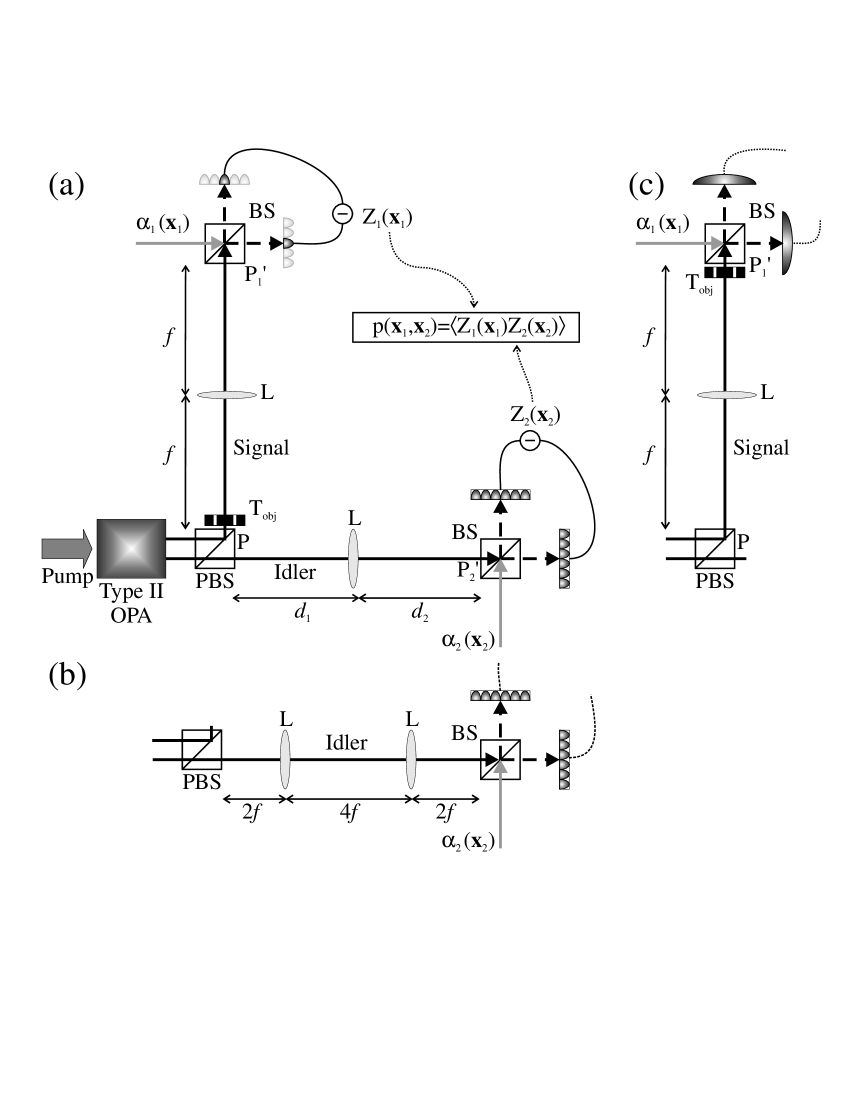
Figure 1: The system setup. Sketch (a) shows the general setup where a point-like detector (or a pixel array) is used in the test (signal) arm. Sketch (b) shows the case of a telescope setup in the reference (idler) arm. Sketch (c) shows the test arm setup when bucket detectors are used for the measurements there. See the text for more details. L: lens of focal length $f$, PBS: polarized beam splitter, BS: beam splitter, $P$: crystal plane, $P_{1}^{\prime}$: signal measurement plane, $P_{2}^{\prime}$: idler measurement plane.

In this publication we will focus mainly on the point-like detector in the signal arm for two reasons. First of all, in the high-gain regime there are many photons per mode implying that a single-pixel measurement carry enough information to perform the correlation. In contrast, in the low-gain regime the probability of having a photon after the object is so low that a bucket detector is sometimes favored in order to get coincidences within a reasonable time. Secondly, having spatial resolution in the signal arm allows to perform averages over the pixels of the test arm detector (in this case it is necessary to have an array of pixels in the test arm), which as we will show vastly speeds up the convergence rate as well as improves the imaging bandwidth. For completeness we also treat the bucket detector case in Sec. V.

We consider the case where the signal and idler input fields are in the vacuum state. Thus, in the SPWPA we have the following correlations at the crystal exit gatti:2003c ; brambilla:2004

$$\langle a_{j}^{\mathrm{out\dagger}}(\vec{q},\Omega)a_{k}^{\mathrm{out}}(\vec{q}^{\prime},\Omega^{\prime})\rangle$$

$$=\delta_{jk}\delta(\vec{q}-\vec{q}^{\prime})\delta(\Omega-\Omega^{\prime})|V_{j}(\vec{q},\Omega)|^{2},\quad j=1,2$$ (14a)

$$\langle a_{1}^{\mathrm{out}}(\vec{q},\Omega)a_{2}^{\mathrm{out}}(\vec{q}^{\prime},\Omega^{\prime})\rangle$$

$$=\delta(\vec{q}+\vec{q}^{\prime})\delta(\Omega+\Omega^{\prime})U_{1}(\vec{q},\Omega)V_{2}(-\vec{q},-\Omega).$$ (14b)

The type II phase matching conditions of the crystal ensure that the signal and idler have orthogonal polarizations and therefore at the exit of the crystal they can be separated by a polarizing beam splitter (PBS). We will neglect the distance between the crystal and the PBS. The fields $c_{j}(\vec{x},t)$ at the measurement planes $P_{j}^{\prime}$ are connected to the output fields at the crystal exit plane $P$ by a Fresnel transformation formally written as

$$c_{j}(\vec{x}_{j},t) = \int d\vec{x}^{\prime}h_{j}(\vec{x}_{j},\vec{x}^{\prime})a_{j}^{\mathrm{out}}(\vec{x}^{\prime},t)+V_{j}(\vec{x}_{j}),$$ (15)

where $h_{j}(\vec{x}_{j},\vec{x}^{\prime})$ are kernels related to the optical path from $P$ to $P_{j}^{\prime}$. $V_{j}(\vec{x}_{j})$ accounts for losses in the imaging system that are linearly proportional to vacuum field operators and therefore uncorrelated to the PDC fields.

The object is described by a transmission function $T_{\mathrm{obj}}(\vec{x})$, and is set in the signal arm. Besides the object the signal arm is set in the so-called f-f imaging scheme, consisting of a lens L with focal length $f$ located at a distance $f$ from both the crystal exit and from the detection plane $P_{1}^{\prime}$. If we apply the unfolded Klyshko picture klyshko:1988 it is obvious that the required position of the object changes depending on the type of detector used in the test arm. Namely, when a point-like detector is used the detector acts like a point-like source which through the f-f lens system becomes plane wave source at the crystal, and therefore the optimal object placement is at $P$, as shown in Fig. 1a. Conversely, if a bucket detector is chosen it acts like a plane wave source at $P_{1}^{\prime}$ and through the f-f lens system it changes to a point-like source at $P$. Thus, if in this case we put the object at $P$ we will not get any information about it, while if we put the object at $P_{1}^{\prime}$ it is instead effectively illuminated by the plane wave source. Thus, in the bucket case the object must be placed at $P_{1}^{\prime}$, as shown in Fig. 1c. Consequently, the signal Fresnel kernels are

$$h_{1}(\vec{x}_{1},\vec{x}^{\prime}) = (i\lambda_{1}f)^{-1}e^{-i\frac{2\pi}{\lambda_{1}f}\vec{x}_{1}\cdot\vec{x}^{\prime}}T_{\mathrm{obj}}(\vec{x}^{\prime}),$$ (16a)

$$h_{1}^{\mathrm{b}}(\vec{x}_{1},\vec{x}^{\prime}) = (i\lambda_{1}f)^{-1}e^{-i\frac{2\pi}{\lambda_{1}f}\vec{x}_{1}\cdot\vec{x}^{\prime}}T_{\mathrm{obj}}(\vec{x}_{1}),$$ (16b)

for the point-like and the bucket detector case, respectively, and the superscript “b” denotes bucket. $\lambda_{1}$ is the wavelength of the signal field. Note that the lens in the signal arm could actually be removed and substituted by a propagation over a distance long enough to be in the Frauenhofer regime. However, the phase of the signal field could be difficult to control in that case.

We will fix the setup of the signal arm once and for all. We may then adjust the idler arm to retrieve the desired kind of information through the signal-idler correlations. The idler lens system also consists of a lens L of focal length $f$, as shown in Fig. 1a. In one setup $d_{1}$ and $d_{2}$ are identical and both equal to the lens focal length, $d_{1}=d_{2}=f$, i.e. an f-f setup as also used in the signal arm. With this setup the correlations in the point-like detector case give information about the object far field, while in the bucket detector case they give information about the object near field. In the other setup, instead, these distances obey the thin lens law $1/d_{1}+1/d_{2}=1/f$. This means that the object near field can be retrieved from the correlations in the point-like detector case, while the object far field can be retrieved in the bucket detector case. For simplicity we may keep $d_{1}=d_{2}=2f$ and we denote this the 2f-2f setup. We will also consider the so-called telescope case, see Fig. 1b, where the 2f-2f setup is repeated twice adding an extra lens, but the system still obeys the thin lens law: therefore the object information can be retrieved as in the 2f-2f case. For these three chosen setups in the idler plane, the idler field at $P_{2}^{\prime}$ is then given by the Fresnel transformation (15) with the kernels

$$h_{2,f}(\vec{x},\vec{x}^{\prime}) = (i\lambda_{2}f)^{-1}e^{-i\frac{2\pi}{\lambda_{2}f}\vec{x}\cdot\vec{x}^{\prime}}\;,$$ (17a)

$$h_{2,2f}(\vec{x},\vec{x}^{\prime}) = e^{-i\frac{\pi}{\lambda_{2}f}|\vec{x}|^{2}}\delta(\vec{x}+\vec{x}^{\prime}),$$ (17b)

$$h_{2,T}(\vec{x},\vec{x}^{\prime}) = \delta(\vec{x}-\vec{x}^{\prime}),$$ (17c)

for the f-f setup, the 2f-2f setup, and the telescope setup, respectively. We choose to work with the telescope setup with respect to the 2f-2f setup because of the direct transformation from the image plane $P$ to the measurement plane $P_{2}^{\prime}$ [due to the $\delta(\vec{x}^{\prime}-\vec{x})$ type correlation], as well as the lack of the phase factor.

The fields at $P_{j}^{\prime}$ are measured using balanced homodyne detection schemes, so $c_{j}(\vec{x}_{j},t)$ is mixed with an LO $\alpha_{j}(\vec{x}_{j},t)$ on a 50/50 beam splitter, and after the beam splitter the two fields are

$$c_{j,\pm}(\vec{x},t)=\frac{c_{j}(\vec{x},t)\pm\alpha_{j}(\vec{x},t)}{\sqrt{2}}.$$ (18)

The LO is treated as a classical coherent field, therefore by measuring the field intensities at the photo-detectors and subtracting them we obtain

$$Z_{j}(\vec{x},t) \equiv c_{j,+}^{\dagger}(\vec{x},t)c_{j,+}(\vec{x},t)-c_{j,-}^{\dagger}(\vec{x},t)c_{j,-}(\vec{x},t)$$ (19)

$$= c_{j}(\vec{x},t)\alpha_{j}^{*}(\vec{x},t)+c_{j}^{\dagger}(\vec{x},t)\alpha_{j}(\vec{x},t)$$

$$= |\alpha_{j}(\vec{x},t)|$$

$$\times [c_{j}(\vec{x},t)e^{-i\phi_{j}^{\mathrm{LO}}(\vec{x},t)}+c_{j}^{\dagger}(\vec{x},t)e^{i\phi_{j}^{\mathrm{LO}}(\vec{x},t)}].$$

Here we have the well known result that by properly adjusting the local oscillator phase $\phi_{j}^{\mathrm{LO}}(\vec{x},t)$ one can measure a particular quadrature component of the field.

We now consider the correlation between two particular quadrature components of the signal and idler fields, $Z_{1}$ and $Z_{2}$, integrated over a finite detection time $T_{d}$

$$p(\vec{x} {}_{1},\vec{x}_{2})=\int_{T_{d}}dt_{1}\int_{T_{d}}dt_{2}\langle Z_{1}(\vec{x}_{1},t_{1})Z_{2}(\vec{x}_{2},t_{2})\rangle$$

$$=\int_{T_{d}}dt_{1}\int_{T_{d}}dt_{2}\alpha_{1}^{*}(\vec{x}_{1},t_{1})\alpha_{2}^{*}(\vec{x}_{2},t_{2})$$

$$\times\langle c_{1}(\vec{x}_{1},t_{1})c_{2}(\vec{x}_{2},t_{2})\rangle+\mathrm{c.c.}$$ (20b)

The last line follows from adopting the parametric approximation as well as from the fact that the signal and idler are in the vacuum state at the crystal entrance, since under these assumptions $\langle c_{1}^{\dagger}(\vec{x}_{1},t_{1})c_{2}(\vec{x}_{2},t_{2})\rangle=0$. In most cases $T_{d}\gg\tau_{\mathrm{coh}}$ so the detector is too slow to follow the temporal dynamics of the system. This means that the measured intensities are in fact proportional to the time-integrated field quadratures selected by the LOs.

In the SPWPA we may evaluate the correlation (20b) using the formalism outlined in Eqs. (8)-(10). We will do this in the degenerate case where signal and idler have identical wavelengths $\lambda_{1}=\lambda_{2}\equiv\lambda$ and hence also vacuum wave numbers $k_{1,\mathrm{v}}=k_{2,\mathrm{v}}\equiv{k_{\mathrm{v}}}=2\pi/\lambda$. In order to evaluate the correlation (20b) we note that Eq. (15) provides the Fresnel transformation from the exit of the crystal to the detection plane. The correlations at the crystal exit are the near field signal-idler correlation which can be found from (14b) as

$$\langle a_{1}^{\mathrm{out}}(\vec{x}_{1},t_{1})a_{2}^{\mathrm{out}}(\vec{x}_{2},t_{2})\rangle=$$

$$\int\frac{d\Omega}{2\pi}e^{-i\Omega(t_{1}-t_{2})}\int\frac{d\vec{q}}{(2\pi)^{2}}e^{i\vec{q}(\vec{x}_{1}-\vec{x}_{2})}G(\vec{q},\Omega),$$ (21)

where we have introduced the gain function

$$G(\vec{q},\Omega)=|G(\vec{q},\Omega)|e^{i\phi_{G}(\vec{q},\Omega)}\equiv U_{1}(\vec{q},\Omega)V_{2}(-\vec{q},-\Omega).$$ (22)

Appendix A shows an approximate quadratic expansion of the gain phase that will become useful in the following.

We now use (15) and (III) to obtain a more useful notation for the signal-idler correlation at the detectors

$$\langle c_{1}(\vec{x}_{1},t_{1})c_{2}(\vec{x}_{2},t_{2})\rangle=\int\frac{d\Omega}{2\pi}e^{-i\Omega(t_{1}-t_{2})}$$

$$\times\int d\vec{q}h_{1}(\vec{x}_{1},-\vec{q})h_{2}(\vec{x}_{2},\vec{q})G(\vec{q},\Omega),$$ (23a)

$$h_{j}(\vec{x},\vec{q})\equiv\int\frac{d\vec{x}^{\prime}}{2\pi}e^{-i\vec{q}\cdot\vec{x}^{\prime}}h_{j}(\vec{x},\vec{x}^{\prime}).$$ (23b)

By using Eq. (23) we may evaluate the signal-idler correlation (20b) for $T_{d}\gg\tau_{\mathrm{coh}}$. The details of this calculation are put in Appendix B, and basically there are two limits to consider. One is the case of a pulsed LO where the LO duration time is much smaller than the coherence time, and the result is given by Eq. (B). The other case is that of a continuous-wave (cw) LO, where the LO duration time is much larger than the coherence time, and the result is given by Eq. (B). As mentioned in the appendix we did not find substantial differences between the two cases, and we therefore decided to use the latter in the rest of this paper for the analytical calculations. For completeness we repeat Eq. (B), stating that for a cw LO the following expression holds

$$p(\vec{x}_{1},\vec{x}_{2})=\frac{T_{d}}{2\pi}\alpha_{1}^{*}(\vec{x}_{1})\alpha_{2}^{*}(\vec{x}_{2})$$

$$\times\int d\vec{q}h_{1}(\vec{x}_{1},-\vec{q})h_{2}(\vec{x}_{2},\vec{q})G(\vec{q},0)+\mathrm{c.c.},$$ (24)

where $\alpha_{j}(\vec{x})\equiv\alpha_{j}(\vec{x},t=0)$.

In the following two sections we treat the two choices for the measurement technique in the signal arm, namely point-like detectors and bucket detectors. In each section both analytical and numerical results are presented.

IV Point-like detector setup in test arm

When point-like detectors are used in the test arm the setup of Fig. 1a is used. The signal arm we keep fixed in the f-f setup with the object at the crystal exit. The idler arm is then set in either the f-f setup or the telescope setup. The information is extracted by fixing the signal detector position $\vec{x}_{1}$ and scanning the idler detector position $\vec{x}_{2}$. This gives a simple, fixed setup of the test arm.

IV.1 Analytical results

The analytical results are based on the SPWPA, so evaluating (23b) for the signal we use (16a) to obtain

$$h_{1}(\vec{x}_{1},\vec{q})=(i\lambda f)^{-1}\tilde{T}_{\mathrm{obj}}(\vec{x}_{1}{k_{\mathrm{v}}}/f+\vec{q}),$$ (25)

where $\tilde{T}_{\mathrm{obj}}(\vec{q})$ is the Fourier transform of $T_{\mathrm{obj}}(\vec{x})$.

IV.1.1 Retrieval of object far field

The object far field can be retrieved from the correlations in the point-like detector case by properly adjusting the optical setup in the reference arm based on the f-f scheme. We therefore evaluate (23b) in the f-f case where by using (17a) we obtain

$$h_{2,f}(\vec{x}_{2},\vec{q})=2\pi(i\lambda f)^{-1}\delta(\vec{q}+\vec{x}_{2}{k_{\mathrm{v}}}/f).$$ (26)

By inserting (25) and (26) in (III) the signal-idler quadrature correlation is

$$p_{f}(\vec{x}_{1},\vec{x}_{2}) = \frac{2T_{d}}{(\lambda f)^{2}}|G(-\vec{x}_{2}{k_{\mathrm{v}}}/f,0)\alpha_{1}(\vec{x}_{1})\alpha_{2}(\vec{x}_{2})|$$ (27a)

$$\times \mathrm{Re}\left(\tilde{T}_{\mathrm{obj}}[(\vec{x}_{1}+\vec{x}_{2}){k_{\mathrm{v}}}/f]e^{i\Phi_{f}(\vec{x}_{1},\vec{x}_{2})}\right),$$

$$\Phi_{f}(\vec{x}_{1},\vec{x}_{2}) \equiv \phi_{G}(-\vec{x}_{2}{k_{\mathrm{v}}}/f,0)$$ (27b)

$$-\phi_{2,f}^{\mathrm{LO}}(\vec{x}_{2})-\phi_{1}^{\mathrm{LO}}(\vec{x}_{1})+\pi.$$

This is the main result for the retrieval of the object far field. We now discuss how to optimize the system for obtaining the far-field image information.

First of all we notice that we need to keep the spatial dependence of the LO moduli as constant as possible, effectively setting a limit on their spatial waists. However, since the effect of the LO moduli is a simple multiplication on the correlation it is easy to do a post-measurement correction of the correlations. This means that matching the spatial overlaps of the LO moduli and the PDC fields should be straightforward, while the phases of the LOs are more crucial, as discussed below. The same comments turn out to hold for the other setups discussed in the paper.

Second of all, when $\vec{x}_{2}$ is scanned the gain modulus comes into play. We choose a non-collinear phase-matching condition (see Sec. IV.2) in which $|G(\vec{q}=-\vec{x}_{2}{k_{\mathrm{v}}}/f,0)|$ is a plateau shaped function centered on $\vec{q}=-\vec{q}_{C}$, with brambilla:2004

$$\vec{q}_{C}=\frac{1}{2}\vec{\rho}_{2}l_{c}q_{0}^{2}=\vec{\rho}_{2}(1/k_{1}+1/k_{2})^{-1}.$$ (28)

Additionally, it is roughly constant over a finite region determined by the spatial bandwidth $q_{0}$ defined by Eq. (12a). This sets a limit to the imaging resolution since the higher order spatial frequency components are cut off by the gain. In Sec. IV.2.3 we will show how to circumvent this limitation.

Finally, the most crucial point is to control the LO phases to observe the desired quadrature components of the object far field. It is seen that the real part of the object far field is obtained if we can make $\Phi_{f}(\vec{x}_{1},\vec{x_{2}})=0$, while if we can make $\Phi_{f}(\vec{x}_{1},\vec{x_{2}})=-\pi/2$ the imaginary part of the object far field is obtained. This can be achieved by engineering $\phi_{2,f}^{\mathrm{LO}}(\vec{x}_{2})$ to cancel the gain phase dependence on $\vec{x}_{2}$ that appears in Eq. (27b). As a good approximation we may take $\phi_{2,f}^{\mathrm{LO}}(\vec{x}_{2})$ constant because the gain phase is a slow function over a region determined by $q_{0}$, and we may therefore evaluate it anywhere inside the gain region, e.g. at the gain center $-\vec{x}_{2}{k_{\mathrm{v}}}/f=-\vec{q}_{C}$. Thus, to see the quadrature corresponding to the real part we should choose

$$\psi_{2,f}^{\mathrm{LO}}=\phi_{G}(-\vec{q}_{C},0)-\phi_{1}^{\mathrm{LO}}(\vec{x}_{1})+\pi.$$ (29)

The quadrature component corresponding to the imaginary part of the object far field object may consequently be observed by adding $\pi/2$ to this value.

We can improve this result by using that, as shown in App. A, the gain phase can be approximated with a quadratic expansion in $\vec{q}$, i.e. $\phi_{G}(\vec{q},0)\simeq\phi_{G}^{(0)}+\vec{\phi}_{G,q}^{(1)}\cdot\vec{q}+\phi_{G,q}^{(2)}|\vec{q}|^{2}$ [see Eq. (63a)]. The linear term $\vec{\phi}_{G,q}^{(1)}$ can be compensated by making the idler LO a tilted wave instead of a plane wave, i.e.

$$\phi_{2,f}^{\mathrm{LO}}(\vec{x}_{2})=\psi_{2,f}^{\mathrm{LO}}+\vec{q}_{2,f}^{\mathrm{LO}}\cdot\vec{x}_{2},$$ (30)

where $\psi_{2,f}^{\mathrm{LO}}$ is a controllable reference phase and the wave number $\vec{q}_{2,f}^{\mathrm{LO}}$ may be applied to the LO by using a grating. We should therefore choose the following value of the LO wave number

$$\vec{q}_{2,f}^{\mathrm{LO}}=-\vec{\phi}_{G}^{(1)}{k_{\mathrm{v}}}/f=\rho_{2}l_{c}\Psi_{g}{k_{\mathrm{v}}}/f\vec{e}_{x}.$$ (31)

The quadratic term $\phi_{G,q}^{(2)}$ may be cancelled by shifting the focusing plane of the idler f-f system $\Delta z$ away from the crystal plane $P$ brambilla:2004 , since this gives (in Fourier space) a Fresnel transformation contribution of $\exp(-i\Delta z|\vec{q}|^{2}/2{k_{\mathrm{v}}})$ on the gain function in Eq. (III). Thus, using such a shift, the phase is approximately

$$\phi_{G,\Delta z}(\vec{q},0) \simeq \phi_{G}^{(0)}+\vec{\phi}_{G}^{(1)}\cdot\vec{q}+(\phi_{G}^{(2)}-\Delta z/2{k_{\mathrm{v}}})|\vec{q}|^{2},$$

and by setting $\Delta z/2{k_{\mathrm{v}}}=\phi_{G}^{(2)}$ the quadratic phase term is exactly cancelled. So we must image a plane inside the crystal since this choice from Eq. (63d) implies

$$\Delta z=-(1/n_{1}+1/n_{2})\Psi_{g}l_{c},$$ (32)

with $\Psi_{g}$ defined in Eq. (62). Now all we need to do is to find the overall reference phase. To observe the quadrature component corresponding to the real part of the object far field we should choose

$$\psi_{2,f}^{\mathrm{LO}}=\phi_{G}^{(0)}-\phi_{1}^{\mathrm{LO}}(\vec{x}_{1})+\pi.$$ (33)

with $\phi_{G}^{(0)}$ given by Eq. (63b). This result, the tilted wave LO (31) and the shift of the focusing plane (32) represent the optimized scheme for accessing the far-field image.

IV.1.2 Retrieval of object near field

The object near field can be observed by using the telescope setup in the reference arm. The idler kernel is then found from (17c) and (23b) as

$$h_{2,\mathrm{T}}(\vec{x}_{2},\vec{q})=(2\pi)^{-1}e^{-i\vec{q}\cdot\vec{x}_{2}}.$$ (34)

Using this in (III) we get

$$p_{T}(\vec{x}_{1},\vec{x}_{2})=\frac{T_{d}\alpha_{1}^{*}(\vec{x}_{1})\alpha_{2}^{*}(\vec{x}_{2})}{2\pi i\lambda f}e^{-i\vec{x}_{1}\cdot\vec{x}_{2}{k_{\mathrm{v}}}/f}$$

$$\times\int\frac{d\vec{q}}{2\pi}e^{-i\vec{q}\cdot\vec{x}_{2}}\tilde{T}_{\mathrm{obj}}(\vec{q})G(\vec{x}_{1}{k_{\mathrm{v}}}/f-\vec{q},0)+\mathrm{c.c.}$$ (35)

The correlation is therefore an integral over the gain function and the object far field. Since the gain modulus is a roughly plateau-shaped function in a region determined by $q_{0}$ that acts as a cut-off of the higher values of $\vec{q}$, and the gain phase dependence is slow within this region, the gain can as a good approximation be pulled out of the integration as a constant evaluated at the center of maximum gain $\vec{q}=-\vec{q}_{C}$. The remaining integral is merely the inverse Fourier transform of the object far field, i.e. simply the object near field and we have

$$p_{T}(\vec{x}_{1},\vec{x}_{2})\simeq\frac{T_{d}|G(-\vec{q}_{C},0)\alpha_{1}(\vec{x}_{1})\alpha_{2}(\vec{x}_{2})|}{\pi\lambda f}$$

$$\times\mathrm{Re}[T_{\mathrm{obj}}(\vec{x}_{2})e^{i\Phi_{T}(\vec{x}_{1},\vec{x}_{2})}],$$ (36a)

$$\Phi_{T}(\vec{x}_{1},\vec{x}_{2})\equiv-\vec{x}_{2}\cdot\vec{x}_{1}{k_{\mathrm{v}}}/f+\phi_{G}(-\vec{q}_{C},0)$$

$$-\phi_{1}^{\mathrm{LO}}(\vec{x}_{1})-\phi_{2,T}^{\mathrm{LO}}(\vec{x}_{2})-\pi/2.$$ (36b)

This is the main result for the retrieval of the object near field. We should stress that it is only an approximate result that neglected a cut-off of the high-frequency components of the object Fourier transform. Thus, image information that relies on large spatial frequency components will not be reproduced by the correlations.

If we can make $\Phi_{T}(\vec{x}_{1},\vec{x}_{2})$ constant and equal zero or $-\pi/2$, the real or imaginary part of the near-field object is observed. The linear contribution in $\vec{x}_{2}$ can be cancelled by making the idler LO a tilted wave in the spirit of Eq. (30), i.e. $\phi_{2,T}^{\mathrm{LO}}(\vec{x}_{2})=\psi_{2,T}^{\mathrm{LO}}+\vec{q}_{2,T}^{\mathrm{LO}}\cdot\vec{x}_{2}$ and choosing

$$\vec{q}_{2,T}^{\mathrm{LO}}=-\vec{x}_{1}{k_{\mathrm{v}}}/f.$$ (37)

In order to observe the real part of the object near field the overall constant reference phase must be chosen to

$$\psi_{2,T}^{\mathrm{LO}}=\phi_{G}(-\vec{q}_{C},0)-\phi_{1}^{\mathrm{LO}}(\vec{x}_{1})-\pi/2.$$ (38)

We may optimize the result (36a) by compensating the quadratic term of the gain phase by taking the imaging plane inside the crystal by the amount (32), in the same way as discussed in the previous section. In this case the idler reference phase should instead be

$$\psi_{2,T}^{\mathrm{LO}}=\phi_{G}^{(0)}-\phi_{1}^{\mathrm{LO}}(\vec{x}_{1})+\vec{x}_{1}\cdot\vec{\phi}_{G}^{(1)}{k_{\mathrm{v}}}/f-\pi/2.$$ (39)

with $\phi_{G}^{(0)}$ and $\vec{\phi}_{G}^{(1)}$ given in Eq. (63).

This concludes the analytical part when point-like detectors are used for measuring the signal quadrature components. We emphasize that the retrieval of information about both the object near field and object far field can be done by solely playing with the optical setup of the reference arm. In the following subsection we show specific examples from numerical simulations that support these results.

IV.2 Numerical results

IV.2.1 General introduction

The numerical simulations presented in this paper take into account the Gaussian profile as well as the pulsed character of the pump. They consisted of solving the equations (II) using the Wigner representation to write the stochastic equations (see brambilla:2004 for more details). At each pump shot a stochastic field was generated at the crystal input with Gaussian statistics corresponding to the vacuum state. Quantum expectation values were obtained by averaging over pump shots. This simulates the quantum behavior of symmetrically ordered operators, and thus the correlations calculated are symmetrically ordered. The system we have chosen to investigate is the setup of a current experiment performed in Como jiang:2003 ; jedrkiewicz:2003 . Thus, we consider a BBO crystal cut for type II phase matching. The pump pulse is at $\lambda_{0}=352$ nm and has $\tau_{0}=1.5$ ps. The crystal length is $l_{c}=4$ mm and the dimensionless gain parameter $\sigma_{p}l_{c}=4.0$. Together with a pump waist of $w_{0}=660~{}\mu$m it corresponds roughly to a pump pulse energy of 200 $\mu$J. The crystal is collinearly phase matched at an angle $\theta=49.05^{\circ}$ of the pump propagation direction with respect to the optical $z$ axis dmitriev:1999 . We used $\theta=48.2^{\circ}$ which gives $\Delta_{0}<0$ and a gain that is plateau shaped over a large region centered on $-\vec{q}_{C}$ as given by Eq. (28).

The correlations typically converged after a couple of thousands repeated pump shots when no spatial information was recorded in the test beam (i.e. using either bucket or point-like detectors there). For this reason it is very time-consuming to do a full 3+1D simulation ($xyt$ propagated along $z$). Instead we chose to model a 2+1D system: a single transverse dimension $x$ along the walk-off direction and the temporal dimension $t$ with propagation along the crystal direction $z$. We will also show simulations where in addition to averaging over shots, a spatial average over $\vec{x}_{1}$ is also performed. In the 2+1D simulations this reduces the number of shots needed by an order of magnitude, while in 3+1D it is possible to average over both transverse directions and a diffraction image can be observed even with only a few shots. Thus this method allows us to calculate the correlations even from a full 3+1D simulation.

The integration along the crystal direction was done in $N_{z}=200$ steps. In the 2+1D simulations the $xt$-grid was chosen to $N_{x}=512$ and $N_{t}=32$, while for the 3+1D simulations we chose $N_{x}=N_{y}=256$ and $N_{t}=32$. $(\vec{x},t)$ were scaled to $x_{\mathrm{coh}}$ and $\tau_{\mathrm{coh}}$, respectively, as given by Eq. (13), while $z$ was scaled to the crystal length $l_{c}$.

We chose to investigate the quantitative behavior of the imaging system with a transmitting double slit as the object, defined in one transverse dimension as

$$T_{\mathrm{obj}}(x)=\left\{\begin{array}[]{ll}0,&\;|x-\delta_{x}|>\frac{a+d}{2},\;|x-\delta_{x}|<\frac{d-a}{2}\\ 1,&\;\frac{d-a}{2}\leq|x-\delta_{x}|\leq\frac{a+d}{2}\end{array}\right.,$$ (42)

where $d$ is the distance between the slit centers, $a$ is the slit width, and $\delta_{x}$ is the object shift from origin. This object only introduces amplitude modulations and does not alter phase information. We take $\delta_{x}\neq 0$ in the numerics to compensate for walk-off effects, so we must choose it properly in order for each slit to see the same gain. The analytical Fourier transform is

$$\tilde{T}_{\mathrm{obj}}(q) = a\sqrt{2/\pi}e^{-i\delta_{x}q}\cos(qd/2)\mathrm{sinc}(qa/2),$$ (43)

where $\mathrm{sinc}(x)=\sin(x)/x$. The shift $\delta_{x}$ alone introduces a nonzero imaginary part. Additionally we will present results using a pure phase double slit abouraddy:2003

$$T_{\mathrm{obj}}(x)=\left\{\begin{array}[]{ll}-1,&\;|x-\delta_{x}|>\frac{a+d}{2},\;|x-\delta_{x}|<\frac{d-a}{2}\\ 1,&\;\frac{d-a}{2}\leq|x-\delta_{x}|\leq\frac{a+d}{2}\end{array}\right..$$ (46)

This object does not alter amplitude information.

In homodyne detection the LO is typically taken from the same source that created the pump. One would first generate the pump through second-harmonic generation (SHG), and before the laser light at the fundamental frequency enters the SHG crystal some of the power is taken out using a beam splitter, and this field is then used for the LOs. The second harmonic at the exit of the SHG process is then the pump for the PDC process. Therefore the LOs have more or less the same energy, shape and duration as the pump pulse entering the PDC setup. Through numerical simulations with Gaussian LOs we confirmed the results indicated in the analytical sections, namely that the effect of a Gaussian shaped LO appears trivially as a multiplication [see Eq. (27a) and (36a)]. Since broader LOs can easily be achieved experimentally using a beam expander, we decided to keep the LOs as plane waves in space. Also this allows to base the interpretation of the results on the physics behind the PDC and keeping in mind that the LOs will only change the result with a multiplication of a Gaussian function. The temporal duration was chosen identical to the pump (1.5 ps), which ensures a good overlap between the pulses grosshans:2001 .

IV.2.2 Averaging over shots

In this section we present numerical results from averaging over repeated shots of the pump pulse, and where the optimization steps discussed in the analytical section were carried out (i.e. cancelling the quadratic and linear phase terms of the gain). We also present semi-analytical calculations performed in Mathematica, which take the analytical formulas from Sec. IV.1 and carry out the optimization steps and in addition take explicitly into account the finite gain.

The fixed position of the signal detectors $\vec{x}_{1}$ must be chosen with care. In the far-field case we must ensure that in Eq. (27a) the object diffraction pattern $\tilde{T}_{\mathrm{obj}}[(\vec{x}_{1}+\vec{x}_{2}){k_{\mathrm{v}}}/f]$ is centered where the gain modulus $|G(-\vec{x}_{2}{k_{\mathrm{v}}}/f,0)|$ has its maximum (which it has at $-\vec{x}_{2}{k_{\mathrm{v}}}/f=-\vec{q}_{C}$). Thus we must choose $x_{1}{k_{\mathrm{v}}}/f=-q_{C}=-8.69$. As for the near-field setup Eq. (35) dictates that also here this position should be used to center the gain over the origin of $\tilde{T}_{\mathrm{obj}}$. Thus, the test arm detector position is unchanged as we pass from the far field to the near field.

Figure 2: The reconstruction of the object far-field distribution using the f-f setup in the idler arm. The numerical signal-idler correlations (open diamonds) were calculated from averaging over 2,000 repeated pump shots. In (a) and (b) $\psi_{2}^{\mathrm{LO}}$ was chosen as to observe the real and imaginary parts, respectively. The thin line shows $\tilde{T}_{\mathrm{obj}}$ from Eq. (43), while the thick line is Eq. (27a) as calculated in Mathematica. Slit parameters: $a=9$ pixels, $d=33$ pixels and $\delta_{x}=23$ pixels, corresponding to $34~{}\mu$m, $123~{}\mu$m and $86~{}\mu$m, respectively, for $f=5~{}$cm. $x_{f}=fq_{0}/{k_{\mathrm{v}}}$.

Let us first take the case of an f-f setup in the idler arm. Figure 2 displays the two quadrature components corresponding to the real and imaginary parts, and this confirms that with this setup we can reconstruct the full phase and amplitude information of the object diffraction pattern from the signal-idler correlations. The open diamonds in the figure are results from the numerical simulation. The results are compared to the analytical result (43) shown with a thin line, as well as a Mathematica calculation (thick line) that effectively plots Eq. (27a). Compared to the analytical object distribution, the numerical simulation shows that only the central part of the image is reconstructed since the high frequency components die out. This is a consequence of the finite gain bandwidth, as it was predicted by Eq. (27a): the Mathematica calculation is based on this equation and it almost coincides with the numerical results. An additional conclusion can be made from this agreement: since the Mathematica result assumes that the pump is a stationary plane wave this implies that the Gaussian profile in space and time of the pump pulse in the numerics does not affect the correlations significantly. This is because the object is in this example very localized so the signal field impinging on it is almost constant. At the end of the section we shall see an example, the pure phase object, where this is not the case.

Figure 3: The reconstruction of the object near-field distribution using the telescope setup in the idler arm. The notation and parameters are the same as in Fig. 2, except the thin line here shows $T_{\mathrm{obj}}$ from Eq. (42) while the thick line is Eq. (35) as calculated in Mathematica. $x_{\mathrm{coh}}=1/q_{0}$.

In Fig. 3 we show that by merely exchanging the f-f setup in the reference arm to the telescope setup, we can reconstruct the object near-field distribution from the signal-idler correlations. Fig. 3 (a) shows the real part which follows the shape of the analytical double slit (42), while the almost zero imaginary part shown in (b) confirms that the object does not alter phase information. The analytical SPWPA result using Mathematica is calculated from Eq. (35) [note that it is the integral over $\vec{q}$ that is calculated analytically and not the approximated version given by Eq. (36a)]. In comparison with the analytical object (thin line) only the basic shape can be recognized from the numerics, while as before the numerics agree very well with the analytical Mathematica result. This again indicates that the finite spatial bandwidth of the gain plays a decisive role in reconstructing the object. Actually, the results from the near-field and the far-field scenarios are linked: the far-field showed a cut-off at high frequency components due to finite gain. Exactly this cut-off in Fourier space is what gives the smooth character of the near-field image: as predicted by Eq. (35) the correlation is an integral over $\vec{q}$ of the gain multiplied with the object far-field, and because the finite gain bandwidth acts as a low-pass filter then it is not possible to reconstruct the sharp edges of the double slit as this would require high-frequency spatial Fourier components.

The ghost-imaging schemes distinguish themselves from the Hanbury-Brown–Twiss (HBT) type schemes hanburybrown:1956 in being able to pertain phase information of the image. In the HBT technique the object is placed in both of the correlated beams. When operated with thermal light the HBT technique can give information about the Fourier transform of $|T_{\mathrm{obj}}|^{2}$, while when operated with PDC beams it can give information about the Fourier transform of $T_{\mathrm{obj}}^{2}$ abouraddy:2002 ; gatti:2004 . Thus, the phase information is either lost or altered in the HBT scheme. Instead, in the ghost-imaging schemes the object is only placed in one of the beams, and from this one may instead reconstruct the Fourier transform of $T_{\mathrm{obj}}$. This holds both for PDC beams as well as for thermal (or thermal-like) beams gatti:2004 .

Figure 4: The reconstruction of a pure phase double slit in (a)-(b) the f-f setup case, and (c)-(d) the telescope case. The notation and parameters are the same as in Figs. 2 and 3, except $10^{4}$ shots are used. Note that the Mathematica results (thick) have been adjusted to take into account the finite shape of the signal field impinging on the object.

As a specific demonstration we used the pure phase double slit (46) as an object, since for this object the HBT scheme will not be able to provide information about the diffraction pattern. Figs. 4 (a) and (b) show the far-field reconstruction with the f-f system in the idler arm, and both the real and imaginary parts follow closely the analytical Fourier transform (thin line). Thus, the scheme is able to reconstruct the Fourier transform of a pure phase object. However, there is a disagreement for the central peak in (a), corresponding to the average value of the real part of the near field: the analytical value actually goes out of the plot range shown. This is due to the fact that ideally the Fourier transform of the chosen phase object has a $\delta$-like behavior here because all the photons are transmitted, whereas in the numerics the signal field impinging on the object has a finite extension. We accommodated for this in the Mathematica calculation by multiplying the phase double slit with a Gaussian fitted to the near-field profile of the signal in the numerics, and as can be seen (thick line) the agreement is now very good. In Figs. 4 (c) and (d) the near-field reconstruction is shown with the telescope setup in the idler arm, and as evidenced in the real part (c) the object image can be successfully reconstructed (the imaginary part is not shown since it was roughly zero). Also here the Mathematica calculations include the same finite size of the signal field and match very well with the numerics. We should stress that the “blurred” shape of the slits is due to the finite gain bandwidth (as in Fig. 3), while the deviation away from the slits from the analytical result [thin line, Eq. (46)] is due to the Gaussian profile of the signal [exactly this latter behavior gives rise to a lower central peak in (a)]. Finally, we also show the modulus of the reconstructed near field (d), and we do this to stress that it actually reveals some features of the double slit. This is a consequence of the finite gain bandwidth of the source which turns the signal-idler fields from being completely incoherent (this is the ideal result in the case of infinite bandwidth) to being partially coherent. Note that in the numerics we had to use more shots than before, otherwise the behavior away from the slits in the near-field case was not too regular. This is a consequence of the more noisy statistics there, as these parts have much lower intensities.

IV.2.3 The spatial average technique

In this section we describe how to improve the speed of the correlation convergence as well as to obtain a much larger imaging bandwidth. The idea is to average the correlations not only over repeated shots but also over the position of the signal detector in a certain way. This implies either using a scanning point-like detector setup or an array of detectors in the test arm. This abandons the idea about keeping the test arm setup as simple as possible, but the benefits of having an increased bandwidth and convergence rate should not be neglected. The technique works for reconstructing the far field, while for the near-field reconstruction this technique cannot be applied for several reasons. Most importantly, the final form of the idler correlation (36a) when averaged over $\vec{x}_{1}$ gives the same result as using a bucket detector, and we already argued in Sec. III through the unfolded Klyshko picture that such a setup does not give any information of the object. Another factor is that $\Phi_{T}(\vec{x}_{1},\vec{x}_{2})$ depends linearly on $\vec{x}_{1}$, see Eq. (36b) and (37). Thus, it is impossible to engineer the phases to observe a given quadrature as $\vec{x}_{1}$ is varied.

For the f-f case, however, the technique is very powerful and it works as follows. Let us take the case where we want to see the real part, and assume we have performed all the optimization steps described in Sec. IV.1.1. The correlation is then

$$p_{f}(\vec{x}_{1},\vec{x}_{2})\propto|G(-\vec{x}_{2}{k_{\mathrm{v}}}/f,0)\alpha_{1}(\vec{x}_{1})\alpha_{2}(\vec{x}_{2})|$$

$$\times\mathrm{Re}\left(\tilde{T}_{\mathrm{obj}}[(\vec{x}_{1}+\vec{x}_{2}){k_{\mathrm{v}}}/f]\right).$$ (47)

A change of coordinate system $\vec{x}\equiv\vec{x}_{1}+\vec{x}_{2}$ and averaging over $\vec{x}_{1}$ as $p_{f,\vec{x}_{1}}(\vec{x})\equiv\int d\vec{x}_{1}p_{f}(\vec{x}_{1},\vec{x})$ gives

$$p_{f,\vec{x}_{1}}(\vec{x})\propto\mathrm{Re}\left[\tilde{T}_{\mathrm{obj}}(\vec{x}{k_{\mathrm{v}}}/f)\right]$$

$$\times\int d\vec{x}_{1}|G[(-\vec{x}+\vec{x}_{1}){k_{\mathrm{v}}}/f,0]\alpha_{1}(\vec{x}_{1})\alpha_{2}(\vec{x}-\vec{x}_{1})|,$$

$$=\mathrm{Re}\left[\tilde{T}_{\mathrm{obj}}(\vec{x}{k_{\mathrm{v}}}/f)\right]$$

$$\times\int d\vec{\xi}|G[\vec{\xi}{k_{\mathrm{v}}}/f,0]\alpha_{1}(\vec{\xi}+\vec{x})\alpha_{2}(-\vec{\xi})|,$$ (48)

where in (48) we have made a change of integration variable $\vec{\xi}\equiv\vec{x}_{1}-\vec{x}$. Assuming that $|\alpha_{1}(\vec{\xi}+\vec{x})|$ is slowly varying with respect to $\vec{\xi}$ in the gain region for any $\vec{x}$ inside the object diffraction pattern, we obtain

$$p_{f,\vec{x}_{1}}(\vec{x})\propto\mathrm{Re}\left[\tilde{T}_{\mathrm{obj}}(\vec{x}{k_{\mathrm{v}}}/f)\right]|\alpha_{1}(\vec{x})|$$

$$\times\int d\vec{\xi}|G[\vec{\xi}{k_{\mathrm{v}}}/f,0]\alpha_{2}(-\vec{\xi})|,$$ (49)

The final integral is just a constant and does not depend on $\vec{x}$, and hence as $\vec{x}$ is scanned the object far field is observed multiplied by the modulus of the signal LO. Thus, whereas with $\vec{x}_{1}$ fixed the imaging system had a finite bandwidth, now the bandwidth is effectively only limited by the shape of the signal LO (which consequently must be taken as broader than the far-field diffraction pattern). Therefore, if we assume that $|\alpha_{1}(\vec{x})|$ has a wide enough profile there is no cut-off of the spatial Fourier frequency components. The possibility of getting rid of the gain cut-off is is relying on the object only being located in one arm so the gain is a function of $\vec{x}_{2}$ only while the object far field is a function of $\vec{x}_{1}+\vec{x}_{2}$. In contrast, if the object is located in both arms, as in the HBT scheme, this would not be possible. Notice that this procedure in practice does not amount to merely integrating over $\vec{x}_{1}$ (as when a bucket detector is used). Rather, one should move to position $\vec{x}_{1}$ of the signal detector while moving together the position $\vec{x}_{2}$ of the idler detector as to keep $\vec{x}=\vec{x}_{1}+\vec{x}_{2}$ constant. This corresponds to a spatial convolution between the signal and idler quadratures. To see that, consider the correlation of the measured quadratures $Z_{j}$, and from Eq. (20) using the substitution $\vec{x}=\vec{x}_{1}+\vec{x}_{2}$ we have

$$p_{f,\vec{x}_{1}}(\vec{x}) = \int_{T_{d}}dt_{1}\int_{T_{d}}dt_{2}$$ (50)

$$\times \int d\vec{x}_{1}\langle Z_{1}(\vec{x}_{1},t_{1})Z_{2}(\vec{x}-\vec{x}_{1},t_{2})\rangle$$

In the numerical simulations this convolution is rapidly calculated using the fast Fourier transform method.

We remark that the bandwidth can also be improved without applying the spatial average. Namely, if instead $\vec{x}_{2}$ is kept fixed and $\vec{x}_{1}$ is scanned, according to Eq. (27a) the gain cut-off is not present, while the diffraction pattern still emerges from the correlations. We performed numerical simulations that showed that this technique in fact gives an unlimited bandwidth as when a spatial average is performed over $\vec{x}_{1}$. However, since no spatial average is performed the convergence rate is as slow as when $\vec{x}_{1}$ is kept fixed. If an average is done over $\vec{x}_{2}$ we obtain the same result as the spatial average over $\vec{x}_{1}$. For a more complete discussion on extending the imaging bandwidth see Ref. bache:2004a .

Figure 5: The same as shown in Fig. 2 except the average is performed over 200 pump shots as well as over $x_{1}$. (a) and (b) show the real and imaginary parts of the reconstructed object far-field. Notice that the full numerical grid is shown. (c) and (d) show the real and imaginary parts of the inverse Fourier transform of the reconstructed far-field correlation function. The thin lines display the analytical results of Eq. (43) for the far field and (42) for the near field.

With the same system setup as in Fig. 2, the result for averaging over all $x_{1}$ is shown in Fig. 5. First of all, we note the excellent agreement between the numerics and the analytical far-field pattern, and also that there is no frequency cut-off: the imaging bandwidth has become practically infinite. Moreover, only 200 shots were needed to obtain the same degree of convergence as in Fig. 2, which is an order of magnitude faster. Another interesting point about homodyne detection is that by measuring both quadratures in the the far-field distribution, we may reconstruct the complete near-field object distribution from this information by using the inverse Fourier transform. We have done this for the data in Fig. 5 (a) and (b) and the result is shown in (c) and (d). The real part, (c), of the inverse Fourier transform follows $T_{\mathrm{obj}}$ very precisely. This is because we now have access to many more high frequency components compared to the case shown in Fig. 3. Thus, as the far-field imaging bandwidth is increased, the near-field resolution improves. It is instructive to note that in the absence of the spatial average the inverse Fourier transform of the far-field correlations shown in Fig. 2 would give exactly the result reported with the telescope setup in Fig. 3. This again underlines the strong link between the near-field and the far-field measurements when all the phase information is intact.

Figure 6: The same setup as used in Fig. 4 except now the average is also done over $x_{1}$. The far-field quadrature correlations are calculated from 1,000 repeated pump shots, and (a) and (b) show the real part and modulus, respectively, of the inverse Fourier transform of the correlation.

Returning to the phase object of Fig. 4 we saw that with the signal detector position fixed the finite gain bandwidth makes the imaging system partially coherent and some phase information is present in the modulus of the correlations. For the phase double slit we repeated the simulations using the spatial average technique to reconstruct the far-field distribution. The inverse Fourier transform of the correlation is shown in Fig. 6 and the real part now shows excellent agreement with the analytical phase double slit (thin line). Most importantly, Fig. 6b showing the modulus now does not reveal any information about the double slit. The extended imaging bandwidth achieved with the spatial average makes the imaging system truly incoherent and hence no phase information is transferred to the modulus.

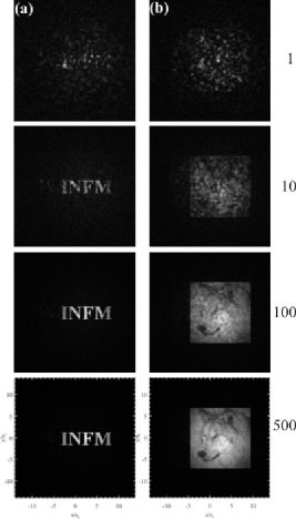
Figure 7: The modulus of the inverse Fourier transform of the far-field correlation function as obtained in an f-f setup with two different objects (a) and (b). The correlations are calculated from a full 3+1D simulation, and averaging over the entire $\vec{x}_{1}$ plane and over the number of repeated pump shots shown on the right.

The spatial average over $\vec{x}_{1}$ works even better in two transverse dimensions because there are many more points to average over. In Fig. 7 we show two cases where different objects were used: (a) a simple amplitude transmission mask with the letters “INFM”, and (b) a more complicated amplitude transmission mask showing a picture of a wolf. The modulus of the inverse Fourier transform of the far-field correlation is shown for different number of shots. Evidently the simple mask (a) converges faster than the more complicated mask (b), but nevertheless in both cases a good, sharp image is obtained after relatively few shot repetitions. After additional averaging over shots the irregularities disappear, as indicated in the last shots.

We now evaluate the qualitative difference of the near-field resolution between the fixed detector case and the spatial average technique. Fig. 8 (a) displays the modulus of the near-field correlations obtained by using the telescope setup and a fixed signal detector position, and Fig. 8 (b) displays the modulus of the inverse Fourier transform of the far-field correlations obtained using the f-f setup and applying the spatial average technique. The blurred character in the fixed detector case that was also present in one transverse dimension (see e.g. Fig. 3) is now very obvious, and does not improve much even if more averages are performed since it is a consequence of the finite bandwidth as mentioned before. In contrast the much improved far-field bandwidth of the spatial average technique increases the near-field resolution so the observed near-field image completely sharp. Note that the simulations in Fig. 8 have been performed neglecting the time dimension, without which a dramatic extension in the amount of computational time would occur. Such an approximation corresponds to using a narrow interference filter, and the approach was justified by comparing the correlations at a fewer number of shots with simulations including also time.

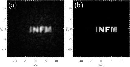
Figure 8: Qualitative comparison of the resolution in (a) the fixed detector case and (b) the spatial average case. (a) uses the telescope setup in the idler arm to obtain the near-field correlation, and the modulus is shown. (b) uses the f-f setup in the idler arm to obtain the far-field correlation, and what is shown is the modulus of the inverse Fourier transform of the correlation. The simulations neglect the time dimension and 5,000 shots are used for the averages.

We have in this section shown that using point-like detectors in the test arm allows to reconstruct both amplitude and phase information about an image. The near-field and far-field object distributions could be obtained by only changing the optical setup of the reference arm. The spatial imaging bandwidth for a fixed test detector position is determined by the source bandwidth, and we showed that this in turn determines the near-field resolution. Using a spatial average technique improves the imaging bandwidth dramatically in the far-field case, and also leads to a much faster information retrieval.

V Bucket detector setup in test arm

We now turn to the case where bucket detectors are used in the test arm. One motivation is to show that by using homodyne detection together with bucket detectors, phase-only objects can be imaged. If an intensity detection scheme is used this is not possible, as shown in Ref. bennink:2002a for the two-photon coincidence imaging case (although it is possible using a point-like detector in the object arm abouraddy:2001 ; abouraddy:2003 ). This is a general result that also holds in the high-gain regime (it can easily be derived from the results of Ref.gatti:2003 ; gatti:2004 ). Another motivation is to see the imaging capabilities of this setup since it technically seems simpler than the point-like detector setup.

V.1 Analytical results

As argued in Sec. III, when bucket detectors are used in the test arm it is necessary to keep the object placed in the measurement plane. Besides that the lens setups in the arms are arbitrary, but we decided to keep the f-f setup in the signal arm, as well as the idler setup in either f-f or the telescope configuration. The test-arm set-up is shown in Fig. 1c. The signal kernel (16b) is transformed according to (23b) as

$$h_{1}^{\mathrm{b}}(\vec{x}_{1},\vec{q}) = \frac{2\pi}{i\lambda f}\delta(\vec{q}+\vec{x}_{1}{k_{\mathrm{v}}}/f)T_{\mathrm{obj}}(\vec{x}_{1}).$$ (51)

The idler kernels remain unchanged. The bucket detectors in the test arm effectively corresponds to an integration over $\vec{x}_{1}$ of the signal-idler quadrature correlation as $\bar{p}_{T}^{\mathrm{b}}(\vec{x}_{2})\equiv\int d\vec{x}_{1}p_{T}^{\mathrm{b}}(\vec{x}_{1},\vec{x}_{2})$.

V.1.1 Retrieval of object near field

For an f-f setup in the reference arm the idler kernel is given by Eq. (26) and from Eq. (III) we therefore obtain

$$p_{f}^{\mathrm{b}}(\vec{x}_{1},\vec{x}_{2}) = \frac{T_{d}}{\pi}\delta(\vec{x}_{1}+\vec{x}_{2})|\alpha_{1}(\vec{x}_{1})\alpha_{2}(\vec{x}_{2})G(\vec{x}_{1}{k_{\mathrm{v}}}/f,0)|$$ (52)

$$\times \mathrm{Re}[T_{\mathrm{obj}}(\vec{x}_{1})e^{i\Phi_{f}^{\mathrm{b}}(\vec{x}_{1},\vec{x}_{2})}],$$

The measured signal-idler correlation is consequently

$$\bar{p}_{f}^{\mathrm{b}}(\vec{x}_{2}) = \frac{T_{d}}{\pi}|\alpha_{1}(-\vec{x}_{2})\alpha_{2}(\vec{x}_{2})G(-\vec{x}_{2}{k_{\mathrm{v}}}/f,0)|$$ (53a)

$$\times \mathrm{Re}[T_{\mathrm{obj}}(-\vec{x}_{2})e^{\bar{\Phi}_{f}^{\mathrm{b}}(\vec{x}_{2})}],$$

$$\bar{\Phi}_{f}^{\mathrm{b}}(\vec{x}_{2}) \equiv \phi_{G}(-\vec{x}_{2}{k_{\mathrm{v}}}/f,0)$$ (53b)

$$-\phi_{1}^{\mathrm{LO}}(-\vec{x}_{2})-\phi_{2,f}^{\mathrm{LO}}(\vec{x}_{2})+\pi.$$

This is the main result for retrieving the near field in the bucket detector case.

The idler LO phase may then be engineered to observe the desired quadrature in much the same way as shown in in Sec. IV.1.1. As a first approximation the gain phase dependence is neglected, so to observe the real part we must have $\bar{\Phi}_{f}^{\mathrm{b}}(\vec{x}_{2})=0$, implying we should choose

$$\psi_{2,f}^{\mathrm{LO}}=\phi_{G}(-\vec{q}_{C},0)-\phi_{1}^{\mathrm{LO}}(-\vec{x}_{2})+\pi.$$ (54)

We may optimize this result by setting the focus plane of the f-f setup in the idler arm inside the crystal with the amount given by Eq. (32) as to compensate the quadratic term of the gain phase. Additionally, by making the idler LO a tilted wave with the wave number given by Eq. (31) we compensate for the linear phase term. With these optimizations, the real part can be observed by choosing

$$\psi_{2,f}^{\mathrm{LO}}=\phi_{G}^{(0)}-\phi_{1}^{\mathrm{LO}}(-\vec{x}_{2})+\pi.$$ (55)

We note that the results show a dependence of the signal LO as $\alpha_{1}(-\vec{x}_{2})$. Therefore, as the idler pixels are scanned it is crucial that the signal LO does not vary substantially. Another point is the scale of the coordinate system, but we will return to this in the next subsection.

V.1.2 Retrieval of object far field

For a telescope setup in the reference arm the idler kernel is given by (34) and thus using Eq. (III) we have

$$p_{T}^{\mathrm{b}}(\vec{x}_{1},\vec{x}_{2})=\frac{T_{d}}{2\pi i\lambda f}\alpha_{1}^{*}(\vec{x}_{1})\alpha_{2}^{*}(\vec{x}_{2})G(\vec{x}_{1}{k_{\mathrm{v}}}/f,0)$$

$$\times T_{\mathrm{obj}}(\vec{x}_{1})e^{-i\vec{x}_{1}\cdot\vec{x}_{2}{k_{\mathrm{v}}}/f}+\mathrm{c.c.}$$ (56)

Thus, the measured correlation is

$$\bar{p}_{T}^{\mathrm{b}}(\vec{x}_{2}) = \frac{T_{d}}{i\lambda f}\alpha_{2}^{*}(\vec{x}_{2})$$ (57)

$$\times \int\frac{d\vec{x}_{1}}{2\pi}e^{-i\vec{x}_{1}\cdot\vec{x}_{2}{k_{\mathrm{v}}}/f}G(\vec{x}_{1}{k_{\mathrm{v}}}/f,0)\alpha_{1}^{*}(\vec{x}_{1})T_{\mathrm{obj}}(\vec{x}_{1})$$

$$+\mathrm{c.c.}$$

We assume now that the plateau-shaped gain and the modulus of the signal LO vary slowly with respect to the object, so they can be taken out of the integral, evaluated at the position of maximum gain $\vec{x}_{1}{k_{\mathrm{v}}}/f=-\vec{q}_{C}$. This approximation yields

$$\bar{p}_{T}^{\mathrm{b}}(\vec{x}_{2})\simeq\frac{2T_{d}}{\lambda f}|G(-\vec{q}_{C},0)\alpha_{1}(-\vec{q}_{C}f/{k_{\mathrm{v}}})\alpha_{2}(\vec{x}_{2})|$$

$$\times\mathrm{Re}[\tilde{T}_{\mathrm{obj}}(\vec{x}_{2}{k_{\mathrm{v}}}/f+\vec{q}_{1}^{\mathrm{LO}})e^{i\bar{\Phi}_{T}^{\mathrm{b}}(\vec{x}_{2})}],$$ (58a)

$$\bar{\Phi}_{T}^{\mathrm{b}}(\vec{x}_{2})\equiv\phi_{G}(-\vec{q}_{C},0)-\psi_{1}^{\mathrm{LO}}-\phi_{2,T}^{\mathrm{LO}}(\vec{x}_{2})+\pi/2.$$ (58b)

This is the main result showing that the object far field can be reconstructed in the bucket detector case.

We can observe the real of the far-field of the object if $\bar{\Phi}_{T}^{\mathrm{b}}(\vec{x}_{2})=0$, which in the case of (58b) implies

$$\phi_{2,T}^{\mathrm{LO}}(\vec{x}_{2})=\phi_{G}(-\vec{q}_{C},0)-\psi_{1}^{\mathrm{LO}}+\pi/2.$$ (59)

As in the other cases the result (58a) can be optimized by compensating for the quadratic gain phase term before the integration by taking the imaging plane of the telescope setup inside the crystal with the amount given by Eq. (32). In that case we should choose the following reference phase for the idler LO to observe the real part

$$\phi_{2,T}^{\mathrm{LO}}(\vec{x}_{2})=\phi_{G}^{(0)}-\psi_{1}^{\mathrm{LO}}+\pi/2.$$ (60)

In connection with optimizing the imaging performance, it is apparent that if the signal LO is a tilted wave then the origin of the reconstructed diffraction pattern changes. This can be used to compensate for undesired walk-off effects by centering the reconstructed image in the place where the idler (which in this setup is in the near field) has its maximum. Additionally, making the idler LO a tilted wave can be used to compensate for unimportant oscillations in the quadrature components that comes from shifting the object near field from origin [see in that connection Eq. (43)].

Let us come back to the scaling of the image information. The particular setup we chose (having the object placed in the far field created by an f-f lens system, just before the bucket detectors) implies that the signal field impinging on the object changes on the scale $x_{f}=fq_{0}/{k_{\mathrm{v}}}$. This is evident in the analytical formulas Eqs. (53b) and (57). In contrast, when the object was placed in the near field the field changed on the scale $x_{\mathrm{coh}}=1/q_{0}$. As an example, for $f=5$ cm and $\lambda=704$ nm, $x_{f}=338~{}\mu$m while in contrast $x_{\mathrm{coh}}=17~{}\mu$m. The consequence is that while imaging is possible with bucket detectors, it occurs on a different (i.e. larger) length scale than with point-like detectors.

V.2 Numerical results

The numerical simulations in the bucket detector case were done exactly as discussed in Sec. IV.2, except now the object is placed after the f-f setup in the test arm. We decided to keep the object structure used in the point-like detector case, i.e. exactly the same number of pixels between the slits as well as for the slit aperture. As discussed above, this means that the slit dimensions are determined by the larger scale $x_{f}$. Moreover, the pure phase double slit in one transverse dimension is used as an object in order to demonstrate the homodyne detection scheme’s capabilities. Finally, we mention that in the numerics all the optimization procedures discussed in the previous sections were carried out. This includes in the telescope case to use a tilted wave signal LO to center the reconstructed diffraction pattern over the peak of the idler near field, as well making the idler LO a tilted wave as to cancel the oscillations in the diffraction pattern originating from centering the object over the signal far-field plateau. These latter two optimizations are not crucial for the imaging performance.

Figure 9: The reconstruction of the object near-field distribution of a pure phase object with bucket detectors in the test arm and using the f-f setup in the reference arm. The numerical correlations (open diamonds) were calculated from averaging over $10^{4}$ pump shots. The thin line is the analytical phase double slit, while the thick line is calculated in Mathematica on basis of Eq. (53a). Slit parameters in pixels as Fig. 2 corresponding for $f=5$ cm to $a=166~{}\mu$m, $d=610~{}\mu$m and $\delta x=-2.9~{}$mm.

Fig. 9 shows the numerical simulation of the reconstruction of the object near field using the f-f setup in the idler arm. The reconstructed real part in (a) follows the analytical double slit, but notice that the Mathematica result (thick line) has a better resolution than the numerical results. This indicates that the finite shape of the pump worsens the resolution, and we will come back to this later. The imaginary part (b) is containing only little information about the slits. Away from the slits the correlations decay to zero because of the finite shape of the far-field gain.

Figure 10: The same as shown in Fig. 9 except now using the telescope setup in the idler arm making it possible to reconstruct the object far-field distribution. The thick line is Eq. (57) calculated in Mathematica while taking into account the finite shape of the idler near-field distribution.

Fig. 10 shows a numerical simulation similar to Fig. 9 but with the telescope setup in the idler arm allowing for the reconstruction of the object far-field distribution. The reconstructed real part in (a) follows within a certain bandwidth the analytical result (thin line). The cut-off is actually caused by the Gaussian shape of the idler near-field profile, which has been taken into account in the Mathematica calculation of the integral (57); without such a correction the Mathematica result would actually very closely follow the analytical result (thin line) without being cut off. This can be understood by inspecting Eq. (57) more closely, since we see that the action of the gain inside the integral is to provide a limit for the object extension. However, in contrast to the point-like detector case of Eq. (27a) where the gain eventually determines the far-field imaging bandwidth, in the bucket case it is not so: Once the object is located inside the gain, the reproduced diffraction pattern is very good. This is also in accord with what we saw in the semi-analytical reproduction of the near field in Fig. 9, where the double slits appear very sharp indicating that the Fourier frequency bandwidth is large. A consequence of this is that if we tailor the pump to have a plane-wave shape, we should see practically no cut-off in the far field as well as a very sharp reproduction of the double slit in the near field. We checked this to be the case. Thus, also the bucket detector case shows an inherent link between far-field bandwidth and near-field resolution. Finally, note that the imaginary part (b) is zero because we chose to eliminate the oscillations arising because of the offset of the object from origin, making the Fourier transform purely real. Additionally, the central peak of the analytical function in (a) goes out of the range shown for the same reasons as in Fig. 4.

In conclusion, a homodyne detection scheme with bucket detectors in the test arm is capable of observing both amplitude and phase distribution of an object. Both the near-field and the far-field distributions are accessible by only changing the optical setup in the reference arm and even phase-only objects can be imaged.

VI Conclusion

We have shown how a homodyne detection technique can be used to get access to both modulus and phase information in ghost-imaging schemes based on parametric down-conversion in the high-gain regime. It is necessary to measure both the signal and idler beams with individual local oscillators, and we have shown analytically how to engineer the phases of these in order to retrieve both the object image (near field) and the object diffraction pattern (far field). The results were confirmed with numerical simulations taking into account a finite shape of the pump pulse.

We showed that the resolution in the near field and the imaging bandwidth in the far field were inherently linked, and were restrained to the finite gain of the source. Thus in the far-field setup the gain cuts off the higher frequency components in the spatial Fourier domain. In the near-field setup the image is more blurred than the reference image, and we showed that this is exactly a consequence of the higher frequency components missing in the spatial Fourier domain because of the gain cut-off.

The homodyne scheme allows us to have access to both phase and amplitude information, implying it is possible to pass from the far-field result to the near-field result by simply making an inverse Fourier transform. Thus by taking the far-field correlations containing the information about the diffraction pattern and performing an inverse Fourier transform gave the same result as measuring the near-field correlations containing the information about the object image, and vice versa. This also means that once we have measured e.g. the far field there is actually no need to also measure the near field.

We showed that in the far-field setup a spatial average technique over the signal detector pixels leads to much faster convergence rate of the correlations (fewer pump-shot repetitions needed) as well as a hugely improved bandwidth of the diffraction pattern. An intuitive explanation of the method is that each far-field mode is uncorrelated to the rest of the modes in the beam, but the strong mode correlation between the signal-idler beams means that for each signal mode an independent correlation can be measured containing the object information. The spatial average then corresponds to averaging over all the modes in the signal beam. This means that much fewer repeated pump shots of the laser are needed before the correlations converge, and this truly exploits the possibility for parallel operations in spatially correlated beams. The increased bandwidth stands out as the true advantage of the technique, however, and it relies on the fact that as we change the test detector position a different part of diffraction pattern is amplified. Thus, as we average over all the positions we effectively also extract information about different parts of the diffraction pattern, resulting in an increased bandwidth. It is important to note that the technique also works when using direct intensity measurements of the fields instead of homodyne detection, both when using PDC beams (as will be discussed elsewhere in a separate publication bache:2004a ) and the thermal-like beams investigated in gatti:2004 . The technique works particularly well in the high-gain regime because the number of signal photons per mode is not small, but should also work in the low-gain regime.

In the time domain the outcome of a homodyne detection is depending strongly on the temporal overlap between the local oscillator and the field to be measured. A question that had to be answered in this paper was therefore how important it is to ensure a proper overlap also in the spatial domain between the local oscillator and the field. The answer in the context of ghost imaging is that it is not crucial. In fact, the analytical results in the plane-wave pump approximation suggest that the near-field shape of the local oscillator is merely multiplied onto the final result. Even the numerical simulations taking a Gaussian shape of the fields into account suggest the same. Another issue entirely is measurements where the quantum efficiency is important (in contrast to here), and in that case undoubtably the spatial overlap becomes more important.

Using an intensity detection scheme the detection time must not be larger than the coherence time, otherwise the background term that contains no image information becomes dominating and the visibility of the image is dramatically decreased saleh:2000 ; gatti:2004 ; gatti:2004b . In contrast, the homodyne detection scheme is not restricted by this because the correlation function is second order in the field operators implying there is no background term. Hence the detection time may be chosen much larger than the coherence time. Additionally, we have shown that the spatial average technique can give a much larger imaging bandwidth than the source itself. This suggests the possibility of using an optical parametric oscillator (OPO) as a source, and using homodyne detection as a measurement protocol. The limited spatial bandwidth of the OPO with respect to PDC could then be circumvented with the spatial average technique, and the homodyne measurements allow a cw operation of the imaging scheme: since there are no problems with image visibility, the measurement time can be taken longer than the coherence time. Thus, one could effectively abandon the involved scheme of using a high-power laser pumping a PDC setup and the complicated task of overlapping LO fields with the signal-idler fields with temporal durations on a pico-second level.

VII Acknowledgments

This project has been carried out in the framework of the FET project QUANTIM of the EU, of the PRIN project MIUR “Theoretical study of novel devices based on quantum entanglement”, and of the INTAS project “Non-classical light in quantum imaging and continuous variable quantum channels”. M.B. acknowledges financial support from the Danish Technical Research Council (STVF).

Appendix A The approximate form of the gain phase

It is useful to obtain an approximate expression for the gain phase $\phi_{G}$ from the expressions (9). We note in this connection that $\Delta_{12}(\vec{q},\Omega)=\Delta_{21}(-\vec{q},-\Omega)\equiv\Delta(\vec{q},\Omega)$ and therefore also $\Gamma_{12}(\vec{q},\Omega)=\Gamma_{21}(-\vec{q},-\Omega)\equiv\Gamma(\vec{q},\Omega)$. Thus, we obtain

$$\phi_{G}(\vec{q},\Omega) = -\Delta_{0}l_{c}+\arctan\left[\frac{\Delta(\vec{q},\Omega)\tanh[\Gamma(\vec{q,\Omega})l_{c}]}{2\Gamma(\vec{q},\Omega)}\right]$$ (61)

$$\simeq -\Delta_{0}l_{c}+\arctan\left[\Psi_{g}\Delta(\vec{q},\Omega)l_{c}\right]$$

$$\simeq -\Delta_{0}l_{c}+\Psi_{g}\Delta(\vec{q},\Omega)l_{c}.$$

The approximation to Eq. (61) is that the gain is large and that the modes inside the gain are phase matched ($\Delta(\vec{q},\Omega)\simeq 0$) making $\Gamma(\vec{q},\Omega)\simeq\sigma_{p}$. We have also introduced a dimensionless phase parameter that is related to the dimensionless gain parameter $\sigma_{p}l_{c}$

$$\Psi_{g}\equiv\frac{\tanh\left(\sigma_{p}l_{c}\right)}{2\sigma_{p}l_{c}}.$$ (62)

For $\sigma_{p}l_{c}\rightarrow 0$ (small gain) $\Psi_{g}\rightarrow 1/2$ while for $\sigma_{p}l_{c}\gg 1$ (large gain) $\Psi_{g}\rightarrow 0$. Now from Eq. (10c) it is evident that $\Delta(\vec{q},\Omega)$ is quadratic in $\vec{q}$ and $\Omega$, so that the gain phase (61) approximately can be written as

$$\phi_{G}(\vec{q},\Omega) \simeq \phi_{G}^{(0)}+\vec{\phi}_{G,q}^{(1)}\cdot\vec{q}+\phi_{G,q}^{(2)}|\vec{q}|^{2}$$ (63a)

$$+ \phi_{G,\Omega}^{(1)}\Omega+\phi_{G,\Omega}^{(2)}\Omega^{2},$$

$$\phi_{G}^{(0)} = \Delta_{0}l_{c}(-1+\Psi_{g}),$$ (63b)

$$\vec{\phi}_{G,q}^{(1)} = -\rho_{2}l_{c}\Psi_{g}\vec{e}_{x},$$ (63c)

$$\phi_{G,q}^{(2)} = -\frac{(n_{1}+n_{2})l_{c}\Psi_{g}}{2n_{1}n_{2}{k_{\mathrm{v}}}},$$ (63d)

$$\phi_{G,\Omega}^{(1)} = (k_{1}^{\prime}-k_{2}^{\prime})l_{c}\Psi_{g},$$ (63e)

$$\phi_{G,\Omega}^{(2)} = (k_{1}^{\prime\prime}+k_{2}^{\prime\prime})l_{c}\Psi_{g}/2,$$ (63f)

where $\vec{e}_{x}$ is a unit vector in the $x$-direction. We shall use these expressions when the optimal phases of the LOs come into question.

Appendix B The signal-idler correlation

Here we present the detailed calculations of the general expressions for the signal-idler correlation (20b).

By using Eq. (23) we see that in the signal-idler correlation (20b) the evaluation of the temporal part only concerns the gain and the LOs, while the spatial image information comes out from the integral over $\vec{q}$ in Eq. (23). To evaluate the temporal part of the correlation we rewrite (20b) as

$$p(\vec{x}_{1},\vec{x}_{2})=\int d\Omega B(\vec{x}_{1},\vec{x}_{2},\Omega)$$

$$\times\int d\vec{q}h_{1}(\vec{x}_{1},-\vec{q})h_{2}(\vec{x}_{2},\vec{q})G(\vec{q},\Omega)+\mathrm{c.c.},$$ (64a)

$$B(\vec{x}_{1},\vec{x}_{2},\Omega)\equiv T_{d}^{2}\int\int\frac{d\Omega^{\prime}d\Omega^{\prime\prime}}{(2\pi)^{2}}\alpha_{1}^{*}(\vec{x}_{1},\Omega^{\prime})\alpha_{2}^{*}(\vec{x}_{2},\Omega^{\prime\prime})$$

$$\times\mathrm{sinc}[(\Omega-\Omega^{\prime})T_{d}/2]\mathrm{sinc}[(\Omega+\Omega^{\prime\prime})T_{d}/2].$$ (64b)

Let us consider the case of a pulsed LO, i.e. evaluate Eq. (64b) for the LO duration much smaller than $\tau_{\mathrm{coh}}$. Additionally taking into account that, as mentioned before, it can be assumed that $T_{d}\gg\tau_{\mathrm{coh}}$ we may use the approximation $T_{d}\mathrm{sinc}[(\Omega\pm\Omega^{\prime})T_{d}/2]\simeq 2\pi\delta(\Omega\pm\Omega^{\prime})$. In this limit we therefore obtain

$$B(\vec{x}_{1},\vec{x}_{2},\Omega)=\alpha_{1}^{*}(\vec{x}_{1},\Omega)\alpha_{2}^{*}(\vec{x}_{2},\Omega),$$ (65)

which means that the correlation is

$$p(\vec{x}_{1},\vec{x}_{2})=\int d\Omega\alpha_{1}^{*}(\vec{x}_{1},\Omega)\alpha_{2}^{*}(\vec{x}_{2},\Omega)$$

$$\times\int d\vec{q}h_{1}(\vec{x}_{1},-\vec{q})h_{2}(\vec{x}_{2},\vec{q})G(\vec{q},\Omega)+\mathrm{c.c.}$$ (66)

In the case of a continuous wave LO, the LO duration is much longer that $\tau_{\mathrm{coh}}$. Thus, the LO corresponds to a quasi-monochromatic wave, i.e. $\alpha_{j}(\vec{x},\Omega)=\delta(\Omega)\alpha_{j}(\vec{x})$. Using this form in Eq. (64b) removes the integration on $\Omega^{\prime}$ and $\Omega^{\prime\prime}$. Then we use that for $T_{d}\gg\tau_{\mathrm{coh}}$ the remaining term $T_{d}[\mathrm{sinc}(\Omega T_{d}/2)]^{2}$ behaves like $2\pi\delta(\Omega)$, implying

$$B(\vec{x}_{1},\vec{x}_{2},\Omega)\simeq\delta(\Omega)\alpha_{1}^{*}(\vec{x}_{1})\alpha_{2}^{*}(\vec{x}_{2})T_{d}/(2\pi),$$ (67)

which means that the correlation is

$$p(\vec{x}_{1},\vec{x}_{2})\simeq\frac{T_{d}}{2\pi}\alpha_{1}^{*}(\vec{x}_{1})\alpha_{2}^{*}(\vec{x}_{2})$$

$$\times\int d\vec{q}h_{1}(\vec{x}_{1},-\vec{q})h_{2}(\vec{x}_{2},\vec{q})G(\vec{q},0)+\mathrm{c.c.}$$ (68)

It is clear that the pulsed case may have a larger gain than the monochromatic case because of the integration over $\Omega$. However, a crucial point to achieve this goal lies in the minimization of the $\Omega$-dependence of the phase in the integrand of Eq. (B). This will in turn maximize the integral regardless of the value of $\vec{q}$. This can be done approximately by putting in a proper temporal delay between the LOs, effectively cancelling the first-order term (63e) of the gain phase. The second-order term cannot easily be cancelled, but we estimate that this term does not contribute much since we have a negligible contribution of this term of $(k_{1}^{\prime\prime}+k_{2}^{\prime\prime})l_{c}\Omega_{0}^{2}/2=(k_{1}^{\prime\prime}+k_{2}^{\prime\prime})/[(k_{2}^{\prime}-k_{1}^{\prime})^{2}l_{c}]=O(10^{-4})$ for the crystal setup we consider (see Sec. IV.2.1 for details on the setup). Numerical simulations showed that a LO optimized in this way as expected enlarged the effective spatial bandwidth. However, the improvement is not substantial and furthermore it requires temporally short pulses (on the order of 20% of the coherence time, or less) which are difficult to obtain experimentally. We therefore decided only to show analytical results in the limit of a continuous wave LO.

References

- (1) D. N. Klyshko, Sov. Phys. JETP 67, 1131 (1988).
- (2) A. V. Belinskii and D. N. Klyshko, Sov. Phys. JETP 78, 259 (1994).
- (3) D. V. Strekalov, A. V. Sergienko, D. N. Klyshko, and Y. H. Shih, Phys. Rev. Lett. 74, 3600 (1995).
- (4) T. B. Pittman, Y. H. Shih, D. V. Strekalov, and A. V. Sergienko, Phys. Rev. A 52, R3429 (1995).
- (5) P. H. S. Ribeiro, S. Padua, J. C. Machado da Silva, and G. A. Barbosa, Phys. Rev. A 49, 4176 (1994).
- (6) P. H. S. Ribeiro, S. Padua, and C. H. Monken, Phys. Rev. A 60, 5074 (1999).
- (7) B. E. A. Saleh, A. F. Abouraddy, A. V. Sergienko, and M. C. Teich, Phys. Rev. A 62, 043816 (2000).
- (8) A. F. Abouraddy, B. E. A. Saleh, A. V. Sergienko, and M. C. Teich, Phys. Rev. Lett. 87, 123602 (2001).
- (9) A. F. Abouraddy, B. E. A. Saleh, A. V. Sergienko, and M. C. Teich, J. Opt. Soc. Amer. B 19, 1174 (2002).
- (10) A. F. Abouraddy, P. R. Stone, A. V. Sergienko, B. E. A. Saleh, and M. C. Teich, quant-ph/0311147 (2003).
- (11) A. Gatti, E. Brambilla, and L. A. Lugiato, Phys. Rev. Lett. 90, 133603 (2003).
- (12) A. Gatti, E. Brambilla, M. Bache, and L. A. Lugiato, Submitted to Phys. Rev. A, quant-ph/0307187 (2004).
- (13) A. Gatti, E. Brambilla, and L. A. Lugiato, Proc. SPIE 5161, 192 (2004).
- (14) R. S. Bennink, S. J. Bentley, and R. W. Boyd, Phys. Rev. Lett. 89, 113601 (2002).
- (15) R. S. Bennink, S. J. Bentley, R. W. Boyd, and J. C. Howell, Phys. Rev. Lett. 92, 033601 (2004).
- (16) A. Gatti, E. Brambilla, L. A. Lugiato, and M. I. Kolobov, Phys. Rev. Lett. 83(9), 1763 (1999).
- (17) E. Brambilla, A. Gatti, L. A. Lugiato, and M. I. Kolobov, Eur. Phys. J. D 15, 127 (2001).
- (18) P. Navez, E. Brambilla, A. Gatti, and L. A. Lugiato, Phys. Rev. A 65, 013813 (2002).
- (19) A. Gatti, R. Zambrini, M. San Miguel, and L. A. Lugiato, Phys. Rev. A 68, 053807 (2003).
- (20) E. Brambilla, A. Gatti, M. Bache, and L. A. Lugiato, Phys. Rev. A 69, 023802 (2004).
- (21) Z. Y. Ou, S. F. Pereira, H. J. Kimble, and K. C. Peng, Phys. Rev. Lett. 68(25), 3663 (1992).
- (22) A. Kuzmich, I. A. Walmsley, and L. Mandel, Phys. Rev. Lett. 85, 1349 (2000).
- (23) R. E. Slusher, P. Grangier, A. LaPorta, B. Yurke, and M. J. Potasek, Phys. Rev. Lett. 59, 2566 (1987).
- (24) B. Yurke, P. Grangier, R. E. Slusher, and M. J. Potasek, Phys. Rev. A 35, 3586 (1987).
- (25) C. Kim and P. Kumar, Phys. Rev. Lett. 73, 1605 (1994).
- (26) F. Grosshans and P. Grangier, Eur. Phys. J. D 14, 119 (2001).
- (27) Y. Jiang, O. Jedrkiewicz, S. Minardi, P. Di Trapani, A. Mosset, E. Lantz, and F. Devaux, Eur. Phys. J. D 22, 521 (2003).
- (28) O. Jedrkiewicz, Y. Jiang, P. Di Trapani, E. Brambilla, A. Gatti, M. Bache, and L. Lugiato, EH5-4-THU, European Quantum Electronics Conference, Munich, Germany ((2003)).
- (29) V. Dmitriev, G. Gurzadyan, and D. Nikogosyan, Handbook of Nonlinear Optical Crystals, vol. 64 of Springer Series in Optical Sciences (Springer, Berlin, 1999).
- (30) R. Hanbury-Brown and R. Q. Twiss, Nature (London) 177, 27 (1956).
- (31) M. Bache, E. Brambilla, A. Gatti, and L. Lugiato, In preparation (2004).