Estimation of a classical parameter with gaussian probes: magnetometry with collective atomic spins

Abstract

We present a theory for the estimation of a classical magnetic field by an atomic sample with a gaussian distribution of collective spin components. By incorporating the magnetic field and the probing laser field as quantum variables with gaussian distributions on equal footing with the atoms, we obtain a very versatile description which is readily adapted to include probing with squeezed light, dissipation and loss and additional measurement capabilities on the atomic system.

External classical perturbations of a quantum system cause changes in the state of the system, and a measurement of a suitable observable provides an estimate of the strength of the perturbation. Atoms are excellent probes for the estimation of, e.g., classical electric and magnetic fields as well as for rotations and accelerations of inertial frames. The formal description of such ultra-sensitive measurements is quite complicated and has only been formulated recently. The main difficulty arises from the fact that the quantum state of the atoms is changed due to both the interaction with the classical perturbation and the measurement process itself which yields a time series of stochastic outcomes. Quantum trajectory theory Carmichael (1993) makes it possible to simulate this stochastic process, and descriptions are available which combine the quantum dynamics and the parameter estimation conditioned on the detection record Mabuchi (1996); Gambetta and Wiseman (2001). Recently, the classical theory of Kalman filters was combined with the quantum trajectory theory Stockton et al. (2003); Geremia et al. (2003), and under the assumption that the quantum state of the atomic system could be treated as a gaussian state of oscillator-like degrees of freedom, and the initial uncertainty about an applied magnetic field could also be described by a gaussian distribution function, analytical expressions for the precision of the estimate of the field were derived. The analysis showed that the probing of the atomic system squeezes the atomic observable and results in a measurement uncertainty that decreases with time $t$ and atomic number $N_{\text{at}}$ as $1/(N_{\text{at}}t^{3/2})$ and not as $1/\sqrt{N_{\text{at}}t}$, as one might have expected from standard counting statistics arguments.

Here, we present an alternative quantum theory for the estimation of a $B$-field by an atomic probe. The idea is to treat both the laser field used to probe the atoms, the atoms themselves, and the classical $B$-field as one large quantum system. Quantum mechanical state reduction associated with measurements then provides directly the estimate for the expectation value and uncertainty for the quantity of interest. Our theory arrives easily at final estimation results, and it readily generalizes to include decay and losses.

We will assume that a gaussian state, fully characterized by expectation values and covariances, describes the laser field, the atoms and the $B$-field, and we will use that the gaussian character of the state is preserved during the evolution due to the interactions and measurements involved. We benefit from the considerable attention given to the transformation of gaussian states under interactions and measurements because this class of states permits a detailed characterization of entanglement issues (see, e.g., Fiurášek (2002); Giedke and Cirac (2002); Eisert and Plenio (2003); Hammerer et al. (2003) and references therein).

We consider a collection of atoms with a spin-1/2 ground state, polarized along the $x$-axis. The $B$-field is assumed to point along the $y$-axis, and it hence causes a Larmor rotation of the atomic spins towards the $z$-axis. A linearly polarized optical probe is transmitted through the gas. The linear probe is decomposed into two circular components, and different couplings to an excited state introduce a phase difference of the two field components and cause a Faraday rotation of the polarization proportional to the population difference between the atomic $m_{z}$ ground states. It is the recording of this rotation that enables us to determine the $B$-field. The atoms are effectively described by a collective spin operator $\bm{J}=\frac{\hbar}{2}\sum_{i}\bm{\sigma}^{(i)}$, and the polarization components of the field are described by a Stokes vector $\bm{S}$. With the initially spin-polarized sample, and the incident field in a linearly polarized state, we may treat $J_{x}$ and $S_{x}$ as classical variables related to the number of atoms $N_{\text{at}}$ and photons $N_{\text{ph}}$ via $\langle J_{x}\rangle=\frac{\hbar N_{\text{at}}}{2}$ and $\langle S_{x}\rangle=\frac{\hbar N_{\text{ph}}}{2}$. When the field is not too close to resonance, we may eliminate the excited states, and the effective Hamiltonian of the atom-light interaction can be written as $H\propto 2\frac{g^{2}}{\hbar\Delta}J_{z}S_{z}$, with $\Delta$ the detuning from resonance. The coupling strength between a single atom and the radiation field (quantized within a segment of length $L=c\tau$ and area $A$) is $g=\sqrt{\frac{\hbar\omega}{Ac\tau\epsilon_{0}}}d/\hbar$ with $d$ the atomic dipole moment and $\hbar\omega$ the photon energy. It is convenient to introduce effective dimensionless position and momentum operators for the non-classical components of the spin and Stokes vector, $x_{\text{at}}=\frac{J_{y}}{\sqrt{\hbar\langle J_{x}\rangle}}$, $p_{\text{at}}=\frac{J_{z}}{\sqrt{\hbar\langle J_{x}\rangle}}$, $x_{\text{ph}}=\frac{S_{y}}{\sqrt{\hbar\langle S_{x}\rangle}}$, $p_{\text{ph}}=\frac{S_{z}}{\sqrt{\hbar\langle S_{x}\rangle}}$ with commutators $[x_{i},x_{j}]=[p_{i},p_{j}]=0,[x_{i},p_{j}]=i\delta_{ij}$. The perfectly polarized atomic state and the laser field polarized along the $x$-direction correspond to the ground state, i.e., a gaussian minimum uncertainty state of the harmonic oscillator associated with these variable.

We assume that the probing of the atoms takes place with a continuous wave field. Such a field can be treated as a succession of beam segments of duration $\tau$ and with a given mean number of photons $N_{\text{ph}}=2\langle S_{x}\rangle/\hbar=\Phi\tau$ in each segment, with $\Phi$ the photon flux. The continuous measurement of the field is then broken down into individual measurements on each segment. The continuous limit is achieved when $\tau\rightarrow 0$ and $N_{\text{ph}}$ in each segment gets correspondingly small. In the limit of small $\tau$, the integral over $\tau$ is equivalent to the application of a coarse grained Hamiltonian given by $H\tau=\hbar\kappa_{\tau}p_{\text{at}}p_{\text{ph}}$ with dimensionless $\kappa_{\tau}=\frac{2g^{2}}{\Delta}\sqrt{\frac{\langle J_{x}\rangle}{\hbar}\frac{\langle S_{x}\rangle}{\hbar}}\tau=\frac{2g^{2}}{\Delta}\sqrt{\frac{\langle J_{x}\rangle}{\hbar}\frac{1}{2}\Phi}\tau^{3/2}$. Due to the $\tau$-dependence of $g$, $\kappa_{\tau}$ is proportional to $\sqrt{\tau}$. When we incorporate the $B$-field coupling to the atoms, $\beta BJ_{y}/\hbar$, with $\beta$ the atomic magnetic moment, the total effective Hamiltonian is given by

$$H\tau=\hbar\left(\kappa_{\tau}p_{\text{at}}p_{\text{ ph}}+\mu_{\tau}Bx_{\text{at}}\right),$$ (1)

with $\mu_{\tau}=\frac{1}{\hbar}\beta\sqrt{\frac{\langle J_{x}\rangle}{\hbar}}\tau$.

We treat the classical $B$-field variable on equal footing with the quantum variables. The Heisenberg equations of motion for the column vector of the five variables ${\bm{y}}=(B,x_{\text{at}},p_{\text{at}},x_{\text{ph}},p_{\text{ph}})^{T}$ yield ${\bm{y}}(t+\tau)=\mathbf{S_{\tau}}{\bm{y}}(t)$ with the transformation matrix

$${\mathbf{S}_{\tau}}=\left(\begin{array}[]{ccccc}1&0&0&0&0\\ 0&1&0&0&\kappa_{\tau}\\ -\mu_{\tau}&0&1&0&0\\ 0&0&\kappa_{\tau}&1&0\\ 0&0&0&0&1\\ \end{array}\right).$$ (7)

The covariance matrix, defined as in Eisert and Plenio (2003); Giedke and Cirac (2002), $\gamma_{ij}=2\text{Re}\left\langle(y_{i}-\langle y_{i}\rangle)(y_{j}-\langle y_{j}\rangle)\right\rangle$ then transforms as

$$\bm{\gamma}(t+\tau)=\mathbf{S_{\tau}}\bm{\gamma}(t)\mathbf{S_{\tau}}^{T},$$ (8)

due to the atom-light and the atom-field interaction. In the gaussian approximation, the system is fully characterized by the vector of expectation values $\langle{\bm{y}}\rangle$ and the covariance matrix $\bm{\gamma}$. We probe the system by measuring the Faraday rotation of the probe field, i.e., by measuring the field observable $x_{\text{ph}}$. Since the photon field is an integral part of the quantum system, this measurement will change the state of the whole system, and in particular the covariance matrix of the residual system of atoms and $B$-field. We denote the covariance matrix by

$$\bm{\gamma}=\left(\begin{array}[]{cc}\mathbf{A_{\gamma}}&\mathbf{C_{\gamma}}\\ \mathbf{C}^{T}_{\gamma}&\mathbf{B_{\gamma}}\\ \end{array}\right),$$ (11)

where the $3\times 3$ sub-matrix $\mathbf{A_{\gamma}}$ is the covariance matrix for the variables ${\bm{y}}_{1}=(B,x_{\text{at}},p_{\text{at}})^{T}$, $\mathbf{B_{\gamma}}$ is the $2\times 2$ covariance matrix for ${\bm{y}}_{2}=(x_{\text{ph}},p_{\text{ph}})^{T}$, and $\mathbf{C_{\gamma}}$ is the $3\times 2$ correlation matrix for $\bm{y}_{1}$ and $\bm{y}_{2}^{T}$. An instantaneous measurement of $x_{\text{ph}}$ then transforms $\mathbf{A_{\gamma}}$ as Fiurášek (2002); Giedke and Cirac (2002); Eisert and Plenio (2003)

$$\mathbf{A_{\gamma}}\mapsto\mathbf{A}^{\prime}_{\gamma}=\mathbf{A}_{\gamma}-\mathbf{C_{\gamma}}(\mathbf{\pi B_{\gamma}}\mathbf{\pi})^{-1}\mathbf{C}^{T}_{\gamma},$$ (12)

where $\mathbf{\pi}=\text{diag}(1,0)$, and where the inverse denotes the Moore-Penrose pseudoinverse, as $(\mathbf{\pi B_{\gamma}\pi})$ is not invertible. Equation (12) is equivalent to the result for classical gaussian random variables derived, e.g., in Maybeck (1979). After the measurement, the field part has disappeared, and a new beam segment is incident on the atoms. This part of the beam is not yet correlated with the atoms, and it is in the oscillator ground state, hence the covariance matrix $\bm{\gamma}$ is updated with $\mathbf{A}^{\prime}_{\gamma}$, $\mathbf{C}^{\prime}_{\gamma}$ a $3\times 2$ matrix of zeros, and $\mathbf{B}^{\prime}_{\gamma}=\text{diag}(1,1)$.

Unlike the covariance matrix update, which is independent of the value actually measured in the optical detection, the vector $\langle\bm{y}\rangle$ of expectation values will change in a stochastic manner depending on the outcome of these measurements. The outcome of the measurement on $x_{\text{ph}}$ after the interaction with the atoms is random, and the actual measurement changes the expectation value of all other observables due to the correlations represented by the covariance matrix. Let $\chi$ denote the difference between the measurement outcome and the expectation value of $x_{\text{ph}}$, i.e., a gaussian random variable with mean value zero and variance 1/2. The change of $\langle\bm{y}_{1}\rangle$ due to the measurement is now given by:

$$\langle{\bm{y}}_{1}\rangle\mapsto\langle{\bm{y}}^{\prime}_{1}\rangle=\langle{\bm{y}}_{1}\rangle+\mathbf{C_{\gamma}}(\mathbf{\pi B\pi})^{-1}(\chi,0)^{T},$$ (13)

where we use that the measurement on $x_{\text{ph}}$ only, leads to the particularly simple form $(\mathbf{\pi}B\pi)^{-1}=\text{diag}(B(1,1)^{-1},0)$, and hence the actual value of the second entrance in the vector $(\chi,0)$ is unimportant.

The gaussian state of the system is propagated in time by repeated use of (8) and the measurement update formulae (12)-(13). This evolution is readily implemented numerically, and the expectation value and our uncertainty about the value of the $B$-field are given by the first entrance in the vector of expectation values $\langle{\bm{y}}_{1}\rangle=\langle B\rangle$ and the (1,1) entrance in the covariance matrix $\mathbf{A}_{\gamma}(1,1)=2(\Delta B)^{2}$.

The above discussion specifies how the parameter estimation can be performed. In the problem at hand, the variable $x_{\text{at}}$ does not couple to $B$ and $p_{\text{at}}$, and we are left with a closed $2\times 2$ system for the reduced covariance matrix of $B$ and $p_{\text{at}}$: $\mathbf{V}=[2(\Delta B)^{2},2(\Delta Bp_{\text{at}})^{2};2(\Delta p_{\text{at}}B)^{2},2(\Delta p_{\text{at}})^{2}]$. In the limit of infinitesimally small steps the update formulae (8)-(12) translate into a differential equation on the matrix Ricatti form

$$\dot{\mathbf{V}}(t)=-\mathbf{D}\mathbf{V}(t)-\mathbf{V}(t)\mathbf{D}^{T}-\mathbf{V}(t)\mathbf{E}\mathbf{V}(t),$$ (14)

with $\mathbf{D}=[0,0;\mu,0]$, $\mathbf{E}=\text{diag}(0,\kappa^{2})$, $\kappa=\kappa_{\tau}/\sqrt{\tau}$, and $\mu=\mu_{\tau}/\tau$. We solve (14) by expressing it in terms of two coupled linear matrix equations $\dot{\mathbf{W}}=-\mathbf{D}\mathbf{W}$, $\dot{\mathbf{U}}=\mathbf{EW}+\mathbf{D}^{T}\mathbf{U}$, $\mathbf{V}=\mathbf{WU}^{-1}$ Stockton et al. (2003), and find the analytical solution for the variance of the magnetic field

$$\Delta B(t)^{2}=\frac{(1+\kappa^{2}t)\Delta B_{0}^{2}}{1+\kappa^{2}t+\frac{2}{3}\kappa^{2}\mu^{2}(\Delta B_{0})^{2}t^{3}+\frac{1}{6}\kappa^{4}\mu^{2}(\Delta B_{0})^{2}t^{4}}$$ (15)

with $\Delta B_{0}^{2}$ the initial variance. In the limit of $\kappa^{2}t\gg 1$, we have $\Delta B(t)^{2}\simeq 6/(\kappa^{2}\mu^{2}t^{3})$ explicitly giving the $1/N_{\text{at}}$ and $1/t^{-3}$ scaling also found in Geremia et al. (2003).

The lower solid curve in Fig. 1 shows the uncertainty of the $B$-field as a function of time. It is worth pointing out that compared with Geremia et al. (2003), not only the spirit in which we deal with $B$ as a quantum variable but also the formal derivation is different. In Geremia et al. (2003), the Kalman filter equation deals with the covariance matrix for the joint estimator of the classical $B$-field and the mean value of the atomic spin component along the $z$-axis. The latter variance is initially zero, because we assume that the mean value is initially known to be zero. Our covariance matrix deals with two quantum observables, and neither have a vanishing variance in the initial state.

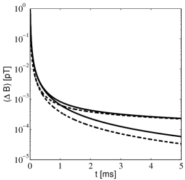
Figure 1: Uncertainty of the $B$-field in pT (1 pT = $10^{-12}$ T) as function of time. We use a 2 mm² interaction area, $2\times 10^{12}$ atoms, $5\times 10^{12}$ photons s^-1, $\Delta B_{0}=1$ pT, 1 GHz detuning, and 852 nm light, appropriate for the ¹³³Cs($6S_{1/2}(F=4)-6P_{1/2}(F=5))$ transition with decay rate $3.1\times 10^{7}$ s^-1 and corresponding atomic dipole moment $d=2.61\times 10^{-29}$ Cm. The effective couplings are $\kappa^{2}=1.83\times 10^{6}$ s^-1 and $\mu=8.79\times 10^{4}$ (s  pT)^-1. Factors of order unity related to the coupling matrix elements among different states of the actual Zeeman substructure are omitted. The lower curves are without inclusion of atomic decay, and the upper curves include atomic spontaneous emission with a rate $\eta=1.7577$ s^-1. The solid (dashed) curves are for coherent (squeezed, $r=3$) optical probe fields (see text).

We may now go back to (13) and derive the stochastic differential equation

$$d\langle B(t)\rangle=\sqrt{2}\kappa(\Delta Bp_{\text{at}})^{2}dW(t)$$ (16)

for the expectation value of the $B$-field. Here $dW(t)=\chi\sqrt{2dt}$ is a Wiener increment with gaussian white-noise statistics $\langle dW(t)\rangle=0$, $\langle dW(t)^{2}\rangle=dt$. $(\Delta Bp_{\text{at}})^{2}\simeq 3/(\kappa^{2}\mu t^{2})$ in the long time limit as determined by the Ricatti equation (14), and it follows that the locking of the value of $\langle B\rangle$, conditioned on the measurements, takes place predominantly in the early stages of the detection process. This is in agreement, of course, with the rapid reduction of the uncertainty as a function of time.

Together with the phase shift, there is a small probability that the atoms decay by spontaneous emission from the upper probe level to one of the two $m_{z}$ ground states. This occurs with a rate $\eta=\Phi\frac{\sigma}{A}\left(\frac{\Gamma^{2}/4}{\Gamma^{2}/4+\Delta^{2}}\right)$, where $\Gamma$ is the atomic decay width and $\sigma=\lambda^{2}/(2\pi)$ is the resonant photon absorption cross-section. The consequence of the decay is a loss of spin polarization. If every atom has a probability $\eta_{\tau}=\eta\tau$ to decay in time $\tau$ with equal probability into the two ground states, the collective mean spin vector is reduced by the corresponding factor $\langle\bm{J}\rangle\rightarrow\langle\bm{J}\rangle(1-\eta_{\tau})$. When the classical $x$-component is reduced this leads to a reduction with time of the coupling strengths $\kappa_{\tau}\mapsto\kappa_{\tau}\sqrt{1-\eta_{\tau}}$ and $\mu_{\tau}\mapsto\mu_{\tau}\sqrt{1-\eta_{\tau}}$, which was also discussed in Geremia et al. (2003); Hammerer et al. (2003), and the vector of expectation values evolves as $\langle\bm{y}(t+\tau)\rangle=\mathbf{L_{\tau}S_{\tau}}\langle\bm{y}(t)\rangle$ with $\mathbf{L_{\tau}}=\text{diag}(1,\sqrt{1-\eta_{\tau}},\sqrt{1-\eta_{\tau}},1,1)$.

The fraction $\eta_{\tau}$ of atoms that have decayed represents a loss of collective squeezing because its correlation with the other atoms is lost, whereas it still provides a contribution $\hbar^{2}/4$ per atom to the collective spin variance. The mean value of $J_{z}^{2}$ can be expressed in terms of the mean values of the $N_{\text{at}}(N_{\text{at}}-1)$ atomic correlations $\sigma_{z}^{i}\sigma_{z}^{j}$, and counting terms, we find that $\langle J_{z}^{2}\rangle\rightarrow(1-\eta_{\tau})^{2}\langle J_{z}^{2}\rangle+(\hbar^{2}N_{\text{at}}/4)(1-(1-\eta_{\tau})^{2})$. Translating this and similar expressions for $J_{y}^{2}$ and $J_{x}J_{y}$ into the appropriate formulae for the effective position and momentum observables, (8) generalizes to

$$\bm{\gamma}(t+\tau)=\mathbf{L_{\tau}}\mathbf{S_{\tau}}\bm{\gamma}(t)\mathbf{S}^{T}_{\tau}\mathbf{L_{\tau}}+\frac{\hbar N_{\text{at}}}{\langle J_{x}(t)\rangle}\mathbf{M_{\tau}},$$ (17)

for $\eta_{\tau}\ll 1$ with $\mathbf{M_{\tau}}=\text{diag}(0,\eta_{\tau},\eta_{\tau},0,0)$. The prefactor $\hbar N_{\text{at}}/\langle J_{x}(t)\rangle$ initially attains the value 2, and increases by the factor $(1-\eta_{\tau})^{-1}$ in each time step $\tau$. The effects of measurements on the covariance matrix and the expectation value vector are obtained as in the case without noise, and for $\eta_{\tau}=0$ we regain the noise-less case.

The upper solid curve in Fig. 1 shows the results of the measurement when noise is taken into account. The covariance matrix makes the atomic probe broader, and simultaneously, the effective coupling of the atoms to the light field and to the $B$-field is reduced, so that the knowledge acquired in the initial detection stages is preserved but the uncertainty $\Delta B$ does not decrease indefinitely.

The value of $B$ is estimated by the polarization rotation of the optical field, and it is natural to enquire whether the use of polarization squeezed light with a smaller variance of $x_{\text{ph}}$ may be utilized to improve the estimate. To analyze this proposal, we go back to our update formulae and represent each new segment of the incident field with gaussian variances $\mathbf{B}^{\prime}_{\gamma}=\text{diag}(1/r,r)$, and leave all other operations unchanged. The result is a reduction of the variance of our estimate, shown as the dashed curves in Fig. 1. The upper dashed curve is for the case when noise is included. The Ricatti equation can be solved in the noise-less case, and the only change of the result in (15) is that all occurrences of $\kappa^{2}$ are replaced by $r\kappa^{2}$. In the long time limit, the estimate is improved by the factor $1/r$. Since the optical field is not squeezed if the time segments $\tau$ are shorter than the squeezing bandwidth $\Omega$, we rely on a separation of time scales $\Omega^{-1}\ll\tau\ll\mu^{-1},\kappa^{-2}$ for the above update formulae to be valid, and for the Ricatti equation to provide a precise analytical solution. For the parameters used in Fig. 1, the squeezing bandwidth should be larger than 10 MHz. Effects of finite squeezing bandwidth will be analyzed elsewhere.

We can improve our estimate by noting that the covariance matrix describes correlations between the atomic observables and the $B$-field, and the uncertainty in the measurement is linked with the uncertainty of the atomic observable $x_{\text{at}}$. After the optical probing it is in principle possible to perform a destructive (Stern-Gerlach) measurement of this atomic variable. This can of course only be done once. The formal treatment of measurements in (12) also applies when the atomic component is being measured, and we can readily determine the new variance on the $B$-field estimate. From the Ricatti equations we know the covariance matrix $\mathbf{A}_{\gamma}$ analytically, and assuming an atomic measurement at time $t$, we obtain $\Delta B_{\text{SG}}(t)^{2}=\frac{(\Delta B_{0})^{2}}{1+2\mu^{2}(\Delta B_{0})^{2}t^{2}+\frac{2}{3}\kappa^{2}\mu^{2}(\Delta B_{0})^{2}t^{3}}$. This variance is smaller than $(\Delta B(t))^{2}$ from (15), and in the long-time limit the variance is reduced by a factor of 4.

In summary, we have described a theory for the estimation of a classical $B$-field by an atomic ensemble with a gaussian distribution of collective spin components. Our theory makes use of results obtained in the study of classification and characterization of entanglement in continuous-variable systems Eisert and Plenio (2003). In general, the gaussian ansatz holds for Hamiltonians which are at most second order polynomials in the canonical variables, and the gaussian character of a system is maintained under physical operations which are implemented using linear optical elements and homodyne measurements Giedke and Cirac (2002). It is clearly convenient to have a unified formalism that deals with both the probing field, the atomic probe, and the unknown $B$-field, and which bypasses the need for separate probabilistic arguments to yield the final estimator. The treatment of the unknown $B$-field as a quantum variable is not incompatible with our assumption that it is a classical parameter. We may imagine a canonically conjugate variable to $B$ having an uncertainty much larger than required by Heisenberg’s uncertainty relation and/or additional physical systems, entangled with the $B$-variable, in which cases the $B$-distribution is indeed incoherent and "classical". Also, one may argue that all classical variables are actually quantum mechanical variables for which a classical description suffices, and hence our theory provides the correct estimator: quantum mechanics dictates that the quantum state provides all the available knowledge about a system, and any estimator providing a tighter bound hence represents additional knowledge equivalent to a hidden variable, and this is excluded by quantum theory. It is of course crucial that our measurement scheme corresponds to a quantum non-demolition (QND) measurement, i.e., we assume that there is not a free evolution of the $B$-field induced by its conjugate variable which may thus remain unspecified. It is also this QND property of the measurement scheme that implies the monotonic reduction of $\Delta B$ which is consistent with the classical parameter estimation (we can not unlearn what we have already learnt about $B$), unlike, e.g., the uncertainty of the atomic $x_{\text{at}}$ variable which must increase when $\Delta p_{\text{at}}$ is reduced and when the atoms undergo spontaneous decay.

We expect extensions of the present theory to be applicable to the description of a variety of experiments aiming at ultra-high precision, including, e.g., atomic clocks, studies of parity violation, and the detection of gravitational waves.

L.B.M. is supported by the Danish Natural Science Research Council (Grant No. 21-03-0163).

References

- Carmichael (1993) H. Carmichael, An Open Systems Aproach to Quantum Optics ((Springer-Verlag, Berlin), 1993).
- Mabuchi (1996) H. Mabuchi, Quant. Semiclass. Opt. 8, 1103 (1996).
- Gambetta and Wiseman (2001) J. Gambetta and H. M. Wiseman, Phys. Rev. A 64, 042105 (2001).
- Stockton et al. (2003) J. K. Stockton, J. M. Geremia, A. C. Doherty, and H. Mabuchi, quant-ph/0309101 (2003).
- Geremia et al. (2003) J. Geremia, J. K. Stockton, A. C. Doherty, and H. Mabuchi, Phys. Rev. Lett. 91, 250801 (2003).
- Fiurášek (2002) J. Fiurášek, Phys. Rev. Lett. 89, 137904 (2002).
- Giedke and Cirac (2002) G. Giedke and J. I. Cirac, Phys. Rev. A 66, 032316 (2002).
- Eisert and Plenio (2003) J. Eisert and M. B. Plenio, quant-ph/0312071 (2003).
- Hammerer et al. (2003) K. Hammerer, K. Mølmer, E. S. Polzik, and J. I. Cirac, quant-ph/0312156 (2003).
- Maybeck (1979) P. S. Maybeck, Stochastic Models, Estimation and Control. Volume 1 (Academic Press: New York, 1979).