Collective effects in the dynamics of driven atoms in a high-Q resonator

Abstract

We study the quantum dynamics of N coherently driven two-level atoms coupled to an optical resonator. In the strong coupling regime the cavity field generated by atomic scattering interferes destructively with the pump on the atoms. This suppresses atomic excitation and even for strong driving fields prevents atomic saturation, while the stationary intracavity field amplitude is almost independent of the atom number. The magnitude of the interference effect depends on the detuning between laser and cavity field and on the relative atomic positions and is strongest for a wavelength spaced lattice of atoms placed at the antinodes of the cavity mode. In this case three dimensional intensity minima are created in the vicinity of each atom. In this regime spontaneous emission is suppressed and the dominant loss channel is cavity decay. Even for a cavity linewidth larger than the atomic natural width, one regains strong interference through the cooperative action of a sufficiently large number of atoms. These results give a new key to understand recent experiments on collective cavity cooling and may allow to implement fast tailored atom-atom interactions as well as nonperturbative particle detection with very small energy transfer.

I Introduction

Cavity quantum electrodynamics CQED using optical resonators has experienced important experimental progress in recent years. Several experimental groups achieved remarkable milestones in the realization of well defined strongly coupled atom-field systems Pinkse04 ; Hood00 ; Pinkse00 ; Mundt02 ; Sauer03 ; KimbleFORT03 ; Kimble95 ; Kuhn02 ; Kimble03a ; MPQ01 ; Horak02 ; Zimmerman03 ; Hemmerich03 ; Chan03 ; Black03 ; Kimble03b . This has lead to numerous applications like single atom trapping by a single photon Pinkse04 ; Hood00 ; Pinkse00 , conditional quantum phase shifts of very weak fields Kimble95 , deterministic sources of entangled photons Kuhn02 ; Kimble03a and a single atom thresholdless laser Kimble03b . Direct observations of the field mode structure MPQ01 ; Horak02 ; Eschner01 and of the mechanical effects of the cavity field on the atomic motion Hood00 ; Pinkse00 ; Juergen03 have been reported culminating in the recent demonstration of cavity induced cooling of single trapped atoms Pinkse04 .

Renewed interest was devoted to large ensembles of atoms commonly coupled to a cavity field with several modes, where collective atomic effects play a central role in the coupled atom-field dynamics Zimmerman03 ; Hemmerich03 ; Chan03 ; Black03 . These experiments have lead to unexpected results and opened new theoretical questions. As a particular example, collective phenomena in the presence of an external transverse driving field involving many atoms at different positions are not fully understood Chan03 ; Black03 .

In this work we study theoretically the dynamics of coherently driven atoms in a resonator. Our investigation takes into account the atomic spontaneous emission, the finite transmittivity of the cavity mirrors and the spatial structure of the cavity mode. The system state is characterized by the atomic fluorescence rate and the signal at the cavity output and studied as a function of the system’s parameter. To get further information on the system, we calculate the probe absorption spectrum and the field distribution in the vicinity of the atoms.

Our results extend the studies of Zippilli04a . There we showed that in the strong coupling regime the system dynamics exhibit enhanced cavity emission accompanied by suppression of fluorescence which occurs, for more than one atom, when the atoms are spatially localized such that they emit in phase into the cavity mode. This phenomenon shares several analogies with the behaviour found in the case of a single atom inside a lossless resonator Alsing92 ; Alsing92a . In fact, this behaviour can be traced back to destructive interference between the laser and the cavity field generated by atomic scattering, such that the atoms couple to a vanishing electric field. As a consequence, we show that the stationary cavity field is independent of the number of atoms and cavity decay becomes the dominant channel of dissipation. In a good cavity this allows to measure the light dissipated through cavity decay without destroying the interference, which is vital if one wants to get information on the cavity field and hence the current atomic positions. In addition, when the strong coupling regime is achieved by a large number of ordered atoms the dynamics we find are consistent with the experimental observations by Vuletic and coworkers Chan03 ; Black03 .

This article is organized as follows. In section II the model is introduced. In section III we review the results obtained for a lossless resonator Alsing92 and investigate the system’s dynamics when the decay rate of the cavity is finite. In section IV the field inside the cavity is investigated by means of (i) an additional weak laser coupled to the atom and (ii) an additional atom weakly coupling to the cavity field. In section V the scaling of the system dynamics with the number of atoms is studied and the results are discussed in connection with the experimental observations in Chan03 ; Black03 . In section VI the results are summarized and discussed, and several outlooks are provided. The appendices report the details of the calculations presented in Secs. III and IV.

II The Model

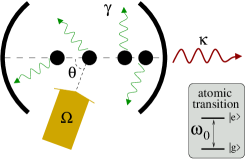
Figure 1: N atoms couple to a 1D optical resonator and are driven transversally by a laser which illuminate them homogeneously. The inset shows the atomic transition which is relevant to the dynamics.

We consider $N$ identical and point-like atoms, whose dipole transitions couple resonantly with the standing-wave mode of an optical resonator. The atoms are assumed to be located along the axis of the resonator, which we denote with the $x$-axis, and their center–of–mass motion is neglected. The relevant atomic degrees of freedom are the ground and excited electronic states $|g\rangle$, $|e\rangle$ of the dipole transition, which is at frequency $\omega_{0}$. The transition couples to the resonator’s mode at frequency $\omega_{c}$ and wave vector $k$, and it is driven by a laser at frequency $\omega_{\rm L}$ and Rabi frequency $\Omega$, as shown in Fig. 1. The laser is assumed to be a classical field. The dynamics of the composite system is described by the master equation for the density matrix $\rho$ of atoms and cavity mode

$$\frac{\partial}{\partial t}\rho=\frac{1}{{\rm i}\hbar}[H,\rho]+{\cal L}\rho+{\cal K}\rho$$ (1)

where $H$ is the Hamiltonian for the coherent dynamics, and ${\cal L}$, ${\cal K}$ are the superoperators describing dissipation due to spontaneous decay and cavity losses. In the reference frame rotating at the laser frequency $\omega_{\rm L}$ the Hamiltonian $H$ has the form

$$H = -\hbar\delta_{c}a^{\dagger}a-\hbar\Delta\sum_{n=1}^{N}|e\rangle_{n}\langle e|$$

$$+ \hbar\sum_{n=1}^{N}\left[g(x_{n})(a\sigma_{n}^{\dagger}+a^{\dagger}\sigma_{n})+\Omega\left({\rm e}^{i\phi_{n}}\sigma_{n}^{\dagger}+{\rm e}^{-i\phi_{n}}\sigma_{n}\right)\right]$$

where $a$, $a^{\dagger}$ are the annihilation and creation operators of a cavity photon; $\sigma_{n}=|g\rangle_{n}\langle e|$, $\sigma_{n}^{\dagger}=|e\rangle_{n}\langle g|$, are the dipole operators for the atom at the position $x_{n}$; $\delta_{c}=\omega_{\rm L}-\omega_{c}$, $\Delta=\omega_{\rm L}-\omega_{0}$ are the detunings of the laser from the frequency of the cavity and of the dipole, respectively. The coupling constant between the dipole at position $x_{n}$ and the cavity mode is $g(x_{n})=g_{0}\cos kx_{n}$, while the coupling with the driving laser depends on the atomic position through the phase $\phi_{n}=kx_{n}\cos\theta$, where $\theta$ is the angle between the cavity axis and the propagation direction of the laser. Finally, the incoherent dynamics is described by the superoperators

$${\cal L}\rho = \frac{\gamma}{2}\sum_{n}\left(2\sigma_{n}\rho\sigma_{n}^{\dagger}-\sigma_{n}^{\dagger}\sigma_{n}\rho-\rho\sigma_{n}^{\dagger}\sigma_{n}\right)$$ (3)

$${\cal K}\rho = \frac{\kappa}{2}(2a\rho a^{\dagger}-a^{\dagger}a\rho-\rho a^{\dagger}a)$$ (4)

where $\gamma$ is the rate of spontaneous emission of the dipole into the modes that are external to the cavity and $\kappa$ is the cavity decay rate. Collective effects in the spontaneous decay are neglected here, as the average distance between the atoms is assumed to be of the order of several wavelengths.

III Enhanced cavity emission in high-finesse cavities

In Alsing92 it has been shown that the steady state of a lossless cavity, coupled to a dipole and driven transversally, is a pure state, such that the energy of the atom and cavity mode is conserved. This regime is accessed when the driving laser is resonant with the cavity mode. Then, the atom is in the ground state and the cavity mode field, generated by atomic scattering, is described by a coherent state whose amplitude is determined by the intensity of the laser. This can be easily seen in Eq. (1) for $\kappa=0$ and $N=1$, after moving to the reference frame described by the unitary transformation

$${\cal D}(\beta)=\exp(\beta a^{\dagger}-\beta^{*}a),$$ (5)

which corresponds to displacing the field inside the cavity by the amplitude $\beta=-\Omega{\rm e}^{{\rm i}\phi}/\bar{g}$ (here, $\bar{g}=g(x)\neq 0$ Footnote:g=0 ). In this reference frame and for $\delta_{c}=0$, Eq. (II) takes the form of the Jaynes-Cummings Hamiltonian and the steady state of the transformed master equation (1) is evidently the state $|g,0\rangle$. In the original reference frame this corresponds to the steady state

$$\rho_{\rm ss}=|g,\beta\rangle\langle g,\beta|$$ (6)

which is a pure state. In fact, the state $|g,\beta\rangle$ is eigenstate of $H$ and is stable for $\kappa=0$. In particular, although the atom is driven both by laser and cavity mode, it is in the ground state as a result of the destructive interference between the atomic excitations induced by the two fields. Therefore, there is no atomic fluorescence and consequentely the only dissipation channel of the system is closed. State (6) exhibits thus the characteristic of a dark state. Moreover, as the atom does not scatter cavity photons and the cavity is assumed to be lossless, the energy of the cavity field is conserved.

In any realistic setup an optical resonator has a finite decay rate $\kappa$. When the atom is driven and $\delta_{c}=0$, the field decay induces dephasing at the atomic position and the state (6) has a finite lifetime. However, it is reasonable to expect Eq. (6) to approximate the steady state for $\kappa$ sufficiently small. In the following, we investigate the intensity of the fluorescence signal and of the signal at the cavity output in different parameter regimes, thereby verifying under which conditions energy dissipation through spontaneous decay can be neglected and when the state inside the cavity can be approximated by a coherent state.

In this section we restrict to the case of one atom and take $g(x)=\bar{g}\neq 0$. The density matrix at time $t$ for $\kappa\neq 0$ can be analytically determined by means of a perturbative expansion in the small parameter $\kappa$, where cavity decay is assumed to be slower than the rate at which the atom reaches the steady state Footnote:1 . At this purpose, we rewrite the master equation (1) in the form

$$\frac{\partial}{\partial t}\rho=\frac{1}{{\rm i}\hbar}\left(H_{\rm eff}\rho-\rho H_{\rm eff}^{\dagger}\right)+J\rho+\kappa{\cal K}_{0}\rho$$ (7)

where

$$H_{\rm eff} = \hbar\bar{g}(a\sigma^{\dagger}+a^{\dagger}\sigma)+\hbar\Omega(\sigma^{\dagger}+\sigma)$$

$$-\hbar\left(\Delta+{\rm i}\frac{\gamma}{2}\right)|e\rangle\langle e|-{\rm i}\hbar\frac{\kappa}{2}a^{\dagger}a$$

and $J\rho=\gamma\sigma\rho\sigma^{\dagger}$, ${\cal K}_{0}\rho=a\rho a^{\dagger}$ are the jump operators. The formal solution of Eq. (7) is Carmichael

$$\rho(t)={\cal S}(t)\rho(0)+\int_{0}^{t}{\rm d}\tau{\cal S}(t-\tau)(J+\kappa{\cal K}_{0})\rho(\tau)$$ (9)

with ${\cal S}(t)\rho(0)=\exp(-{\rm i}H_{\rm eff}t/\hbar)\rho(0)\exp({\rm i}H_{\rm eff}^{\dagger}t/\hbar)$. The perturbative expansion of Eq. (9) at second order in $\kappa$ is reported in Appendix A. The photon scattering rate at time $t$ by the atom into the modes of the continuum is $I_{\rm at}=\gamma{\rm Tr}\{\sigma^{\dagger}\sigma\rho(t)\}$, and grows quadratically with $\kappa$. At the cavity ouput the rate of photon scattering $I_{\rm cav}=\kappa{\rm Tr}\{a^{\dagger}a\rho(t)\}$ at time $t$ and in lowest order is linear in $\kappa$ and $I_{\rm cav}\gg I_{\rm at}$. An instructive case is found in the limit $\Delta=0$ and $\bar{g}\gg\gamma$. Here, these expressions acquire the simple form

$$I_{\rm at}\approx\kappa\frac{\Omega^{2}}{\bar{g}^{2}}\frac{1}{2C_{1}}$$ (10)

$$I_{\rm cav}\approx\kappa\frac{\Omega^{2}}{\bar{g}^{2}}\left(1-\frac{1}{2C_{1}}\right)$$ (11)

where $C_{1}=2\bar{g}^{2}/\gamma\kappa$ is the cooperativity parameter per atom Kimble94 . Thus, the two signals depend on $\kappa$ through the cooperativity parameter $C_{1}$ and the factor $\kappa\Omega^{2}/\bar{g}^{2}$, which is the decay rate of a cavity with mean photon number $\langle n\rangle=\Omega^{2}/\bar{g}^{2}$. From Eqs. (10) and (11) it is visible that for $C_{1}\gg 1$ the fluorescence signal is orders of magnitude smaller than the intensity at the cavity output.

Figure 2 displays $I_{\rm at}$ and $I_{\rm cav}$ as a function of $\kappa$ and for two different values of $\bar{g}$. The curves have been calculated by solving numerically (7). Here, for a wide range of values of the cavity decay rate $I_{\rm cav}$ exhibits a linear behaviour as a function of $\kappa$, while $I_{\rm at}$ is quadratic. Moreover, when $\bar{g}$ is increased (and thus when the cooperativity parameter is increased) the relation $I_{\rm at}\ll I_{\rm cav}$ is fulfilled for a wider range of values of $\kappa$, as it is visible by comparing Fig 2(a) with Fig 2(b). In particular, for $\bar{g}=10\gamma$ the signal $I_{\rm cav}$ largely exceeds the fluorescence signal $I_{\rm at}$ even for $\kappa>\gamma$.

Figure 2: $I_{\rm cav}$ (dashed line) and $I_{\rm at}$ (solid line) as a function of $\kappa$ in units of $\gamma$. Here, $\Omega=\gamma$, $\Delta=\delta_{c}=0$ and (a) $g(x)=\gamma$, (b) $g(x)=10\gamma$. The orizontal dashed-dotted line gives the rate of fluorescence of the atom in free space.

The zero-time correlation function $g^{(2)}(0)$ of the signal at the cavity mirror gives further insight into the dynamics of the cavity field. Figure 3(b) displays $g^{(2)}(0)$ as a function of $\kappa$ and Fig. 3(a) displays the corresponding average number of cavity photons $\langle a^{\dagger}a\rangle$. From these figures one sees that the cavity field exhibits a Poissonian behaviour for a fairly wide range of values of $\kappa$, corresponding to large cooperativity parameters. This behaviour is verified even when the average number of cavity photons is very small (solid line in Fig. 3(a) and (b)). It shows that the cavity mode is in a coherent state, independently of the average energy of the cavity field. This behaviour contrasts dramatically with the antibunching observed when the pump is set directly on the cavity Kimble94 ; Brecha99 .

Figure 3: (a) Mean number of cavity photon and (b) second-order correlation function $g^{(2)}(0)$ as a function of $\kappa$ in units of $\gamma$. Here, $\Delta=\delta_{c}=0$, $\Omega=\gamma$ and $g(x)=\gamma$ (dashed line), $g(x)=10\gamma$ (solid line).

IV Probing the system

In this section we investigate the response of the system to a weak probe in the parameter regime for which the steady state is given to good approximation by state (6). We restrict to the case of one atom, whose dipole transition couples to the driving field and to the cavity mode, and consider the spatial dependence of the coupling. The resonator’s mode function is a standing wave with $g(x)=g_{0}\cos kx$ and the atom is assumed to be at position $x$ such that $g(x)=\bar{g}\neq 0$. The laser is a plane wave, and its phase $\phi_{n}$ depends on the atomic position $x_{n}$ through the relation $\phi(x)=kx\cos\theta$, where $\theta$ is the angle between the direction of propagation of the laser and the cavity axis. We assume that laser and cavity are resonant, and analyze the system’s response to two types of probe: (i) a weak laser field, coupling to the atomic dipole, as shown in Fig. 4; (ii) a second atom of a different species, whose dipole transition frequency is far–off resonance from the cavity frequency, thereby negligibly perturbing the system.

IV.1 Excitation spectrum

We consider a probe driving the atom as illustrated in Fig. 4(a) and evaluate the excitation spectrum, namely the rate of photon scattering into the modes external to the cavity, as a function of the detuning $\delta_{P}=\omega_{P}-\omega_{L}$ of the probe frequency $\omega_{P}$ from the pump.

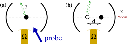
Figure 4: (a) Excitation spectrum: A weak probe is coupled to the atomic dipole and its frequency is scanned through atomic resonance. The fluorescence signal is measured as a function of the probe detuning. (b) A second atom of another species, weakly coupled to cavity and pump fields, probes the cavity field inducing a position-dependent phase shift on the cavity field. The phase shift can be measured by means of homodyne detection or by measuring the fluorescence of the second atom.

For $\delta_{c}=0$ and $\kappa=0$, the scattering rate of probe photons is evaluated for a probe Rabi frequency $\tilde{\Omega}_{P}$ such that $\tilde{\Omega}_{P}\ll\bar{g},\Omega,\gamma$. The details of the calculation are reported in Appendix B. The excitation spectrum is given by

$$w(\delta_{P})=\gamma\hbar\tilde{\Omega}_{P}^{2}\frac{\delta_{P}^{2}}{[\delta_{P}(\delta_{P}+\Delta)-\bar{g}^{2}]^{2}+\delta_{P}^{2}\gamma^{2}/4}$$ (12)

and it is plotted in Fig. 5 for two different values of the detuning $\Delta$ between atom and laser. From Eq. (12) it is evident that $w(\delta_{P}$) vanishes at $\delta_{P}=0$. This behaviour gives rise to a Fano–like profile of the excitation spectrum as a function of $\delta_{P}$ Lounis92 , which is visible in Fig. 5. This profile is a manifestation of destructive interference between the excitation paths contributing to the atomic dynamics, which can be identified with the absorption of photons from the laser and from the cavity field Rice96 . Interference is at the origin of the two resonances visible in Fig 5 where the rate of photon scattering is maximum. They correspond to values of the probe detuning $\delta_{P}=\delta_{\pm}$, with

$$\delta_{\pm}=\frac{1}{2}\left(-\Delta\pm\sqrt{\Delta^{2}+4\bar{g}^{2}}\right),$$

and have width $\gamma_{\pm}$, which for $\sqrt{\Delta^{2}+\bar{g}^{2}}\gg\gamma/2$ take the simple form

$$\gamma_{\pm}\approx\frac{\gamma}{4}\left(1\pm\frac{|\Delta|}{\sqrt{\Delta^{2}+4\bar{g}^{2}}}\right)$$ (13)

In the strong coupling regime these resonances correspond to the dressed states of the atom-cavity system, and their widths determine the characteristic time–scales of the system’s dynamics. Thus, for $\kappa\neq 0$ enhanced cavity emission accompanied by suppression of fluorescence are achieved when ${\rm min}(\gamma_{+},\gamma_{-})>\kappa$.

It is remarkable that $w(\delta_{P})$ does not depend on $\Omega$ and thus does not depend on the average number of photons inside the cavity. In particular, the position and width of the resonances are the ones found for an atom in an empty cavity. This result can be simply explained by observing that the field at the atomic dipole vanishes. In other words, in the reference frame described by the unitary transformation (5) the absorption of a probe photon induces a transition $|g,0\rangle\to|e,1\rangle$, whereby $|e,1\rangle$ is the superposition of the eigenstates of the system at frequencies $\delta_{\pm}$ corresponding to the resonances of the excitation spectrum. For $\kappa\neq 0$ we have verified that also the splitting at the cavity output depends on $g(x)$ and not on $\Omega$. This property suggests a use of this interference effect in order to probe the atomic position inside the cavity without significantly perturbing the system.

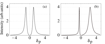
Figure 5: Excitation spectrum $w(\delta_{P})$ as a function of the probe detuning $\delta_{P}$ in units of $\gamma$, for the parameters $g(x)=\gamma$, $\delta_{c}=0$, $\kappa=0$ and (a) $\Delta=0$, (b) $\Delta=-2\gamma$.

IV.2 A second atom probing the cavity field

The electric field inside the cavity can be probed by means of an atom which is weakly coupled, as shown in Fig. 4(b). This can be, for instance, an atom of other species whose dipole transition frequency is far–off resonance from the cavity and the driving laser. This atom thus experiences a small a.c.–Stark shift $\delta_{\rm atom}$, whose intensity is a function of the distance $d=x^{\prime}-x$ from the atom which pumps the cavity. It can be measured with an homodyne detection of the cavity output field, where the pump field is the local oscillator, or by measuring the fluorescence of the probe atom. The shift $\delta_{\rm atom}$ is plotted in Fig. 6 as a function of the distance $d$ for different values $\kappa$. We observe that cavity decay tends to cancel the spatial modulation of the total electric field, which never vanishes inside the cavity for $\kappa\neq 0$. If the mechanical effects of light are considered, then Fig. 6 corresponds to the potential that the probing atom experiences. Hence, the latter may feel a binding or repulsive force in the vicinity of the first atom, depending on the sign of the detuning $\Delta_{2}$ of the laser from the probing atom resonance.

Figure 6: a.c.–Stark shift $\delta_{\rm atom}$ of the probing atom as a function of the distance from the atom pumping the cavity, which is at an antinode of the standing wave. Here, $g_{0}=\Omega=\gamma$, $\Delta=\delta_{c}=0$, and the laser propagation direction is perpendicular to the cavity axis. The detuning of the probe atom from the cavity frequency is $\Delta_{2}=1000\gamma$. Solid line: $\kappa=0$; Dashed line: $\kappa=\gamma$; Dash-Dotted line: $\kappa=2\gamma$.

V Scaling with the number of atoms

V.1 Two atoms inside the resonator

So far we have considered that only one atom couples to the cavity mode. If a second atom of the same kind is inside the cavity and is illuminated by the laser, the dynamics is in general non-trivial. For $\kappa=0$ suppression of fluorescence is observed when the atoms are at a distance $\Delta x$ which is an integer multiple of the wave length $\lambda$. When this occurs, the two atoms are coupled with the same coupling constant $\bar{g}$ to the cavity mode, and from Eq. (1) it can be verified that the state $|g_{1},g_{2},\beta\rangle$ is the steady state of the system with $\beta=-\Omega/\bar{g}$. Hence, the total electric field vanishes at both atoms, while the cavity field is the same as when only one atom couples to the resonator. In general, one can define the function

$$\beta(x)=\Omega(x)\exp({\rm i}(\pi+kx\cos\theta))/\bar{g},$$ (14)

where $\bar{g}=g(x)\neq 0$ and which includes inhomogeneity of the pumping field. Then, the condition for suppression of fluorescence with two atoms is fulfilled whenever two positions exist such that $\beta(x_{1})=\beta(x_{2})$, where the atoms are located. Clearly, there may exist parameters regimes for which function (14) is not periodic and a non-trivial solution for suppression of fluorescence with more than one atom does not exist.

Figures 7 and 8 display the average number of photons and the excited state populations as a function of the relative distance between the atoms, assuming that one atom is fixed at the antinode of the standing wave and that both atoms are homogeneously driven by the laser, which propagates perpendicularly to the cavity axis, i.e. $\theta=\pi/2$. Here it is visible that the excited state population of both atoms vanishes at $x_{2}=0,\lambda$. At these points the field inside the cavity is different from zero, and it is a local minimum as a function of $x_{2}$, as it is particularly evident in Fig 7. The population of the first atom vanishes as well when the second atom is at a node of the standing wave. In this case, the dynamics of the cavity are determined by the coupling with the atom at $x_{1}$, whereas the population of the second atom is determined by the laser intensity, as if it were in free space.

Figure 7: (a) mean number of photons and (b) excited state population of atom at $x_{1}$ (solid line) and at $x_{2}$ (dashed line) as a function of $x_{2}$. Here, $x_{1}$ is an antinode of the standing wave $g(x)=g_{0}\cos kx$. The parameters are $\kappa=0.2\gamma$, $\Omega=\gamma$, $g_{0}=10\gamma$, $\Delta=100\gamma$, $\delta_{c}=0$, and the laser propagation direction is perpendicular to the cavity axis.

Note that Fig. 7 displays the situation when the atoms are driven below saturation. Here both scatter coherently into the cavity mode and a second type of interference effect occurs for $x_{2}=\lambda/2$: At this point the cavity field vanishes, while the atomic populations are equal and different from zero. In fact, for $x_{2}=\lambda/2$ and below saturation the atoms scatter coherently into the cavity mode with opposite phase. At saturation, on the other hand, the scattered light is mostly incoherent, and the cavity field does not vanish at this point, as shown in Fig. 8.

Figure 8: Same as Fig. 7. Here, $\kappa=0.01\gamma$, $\Omega=\gamma$, $g=10\gamma$, $\Delta=\delta_{c}=0$, and the laser propagation direction is perpendicular to the cavity axis.

In Fig. 9 the ratio between the cavity and fluorescence signal is displayed for the case illustrated in Fig. 7 when the atoms are driven below saturation and the laser is orthogonal to the cavity axis. Here one sees clearly that this ratio is maximum when the atoms are a wavelength apart, namely where the function (14) assumes the same value at the atomic positions. For $\kappa\neq 0$ absolute maxima are found when the atoms are at the antinodes of the cavity mode, where the cooperativity parameter is largest and the total electric field vanishes.

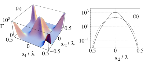
Figure 9: (a) Ratio $\Gamma=I_{\rm cav}/I_{\rm at}$ for two atoms as a function of their position $x_{1}$ and $x_{2}$ inside the cavity for the same parameters as in Fig. 7. (b) Ratio as in (a) as a function of $x_{2}$ for $x_{1}=0$. The dashed line shows $\Gamma$ for the same parameters but $\kappa=\gamma$. Note that $x_{1},~{}x_{2}$ are plotted modulus $\lambda$, and $x_{1}\neq x_{2}$.

These considerations can be extended to three dimensions in a straightforward way. The three-dimensional pattern is found taking into account the phase of the pump, which we always assume to be orthogonal to the cavity axis. The zeros of the electric field are then distributed according to a Body-Centered-Cubic lattice with distance $\lambda/2$ between adiacent planes Domokos02 ; Black03 . Fluorescence is suppressed when the atoms are localized at these points, thus forming a stationary pattern.

V.2 N atoms inside the resonator

The dynamics of the coupled system for generic parameters and number of atoms are very complex. Nevertheless, insight can be gained in the limit in which the atoms are driven below saturation. This assumption enables one to adiabatically eliminate the atomic degrees of freedom from the cavity equation, and corresponds to the parameter regime $|\gamma/2+{\rm i}\Delta|\gg\sqrt{N}g,~{}\sqrt{N}\Omega$, when the collective dipole is driven below saturation. Under these conditions the density matrix of the field $\rho_{\rm f}$ obeys the equation

$$\frac{\partial\rho_{\rm f}}{\partial t}=\frac{1}{2}(\gamma^{\prime}+\kappa)\left\{2a\rho_{\rm f}a^{\dagger}-a^{\dagger}a\rho_{\rm f}-\rho_{\rm f}a^{\dagger}a\right\}$$ (15)

$$+{\rm i}\delta^{\prime}[a^{\dagger}a,\rho_{\rm f}]-{\rm i}[(\xi a^{\dagger}+\xi^{*}a),\rho_{\rm f}]$$

where $\gamma^{\prime}(N)=Ns\gamma$ is the cavity decay rate due to photon scattering by spontaneous emission, $\delta^{\prime}(N)=\delta_{c}-Ns\Delta$ contains the a.c.-Stark shift due to the medium, and $\xi$ is the cavity drive mediated by the dipoles,

$$\xi=Ns\left(\Delta-{\rm i}\frac{\gamma}{2}\right)\frac{\sum_{n}g(x_{n})\Omega e^{i\phi_{n}}}{\sum_{n}|g(x_{n})|^{2}}$$ (16)

Here, $s=\sum s_{n}/N$ where $s_{n}$ is defined for the atom $n$ as

$$s_{n}=\frac{g(x_{n})^{2}}{(\gamma/2)^{2}+\Delta^{2}}$$ (17)

From Eq. (15) it is visible that the system dissipates with rate $\gamma^{\prime}+\kappa$, which determines the rate at which the steady state is reached. The steady state of (15) is $\rho_{\rm f,ss}=|\alpha\rangle\langle\alpha|$, where $|\alpha\rangle$ is a coherent state with amplitude

$$\alpha = -\frac{{\rm i}\xi}{(\gamma^{\prime}(N)+\kappa)/2+{\rm i}\delta^{\prime}(N)}$$

$$= -\Omega\frac{\sum_{n}g(x_{n}){\rm e}^{{\rm i}\phi_{n}}}{\sum_{n}|g(x_{n})|^{2}}\frac{(\gamma/2+{\rm i}\Delta)}{(Ns\gamma+\kappa)/2-{\rm i}(\delta_{c}-Ns\Delta)}$$

and which is the sum of the electric fields scattered at each atom. In fact, in this regime the collective dipole is driven well–below saturation and radiation is scattered elastically into the cavity mode.

For a large number of atoms the contributions of each atom sum up so that the field amplitude $\alpha$ exhibits a narrow peak at the maximum value $\alpha_{0}$ as a function of the mean square deviation of the phase $\Delta\phi_{n}$. This maximum corresponds to the case when all atoms scatter in phase, namely when they are distributed at the points $\{x_{1},\ldots,x_{N}\}$ where the function (14) acquires the same value. The necessary condition that this situation is verified is that $\beta(x)$ is periodic, as we have previously observed. In the following we assume that the laser propagates perpendicularly to the cavity axis, i.e. $\theta=\pi/2$. Hence, $\beta(x)$ has periodicity equal to $\lambda$. Assuming that the atoms scatter in phase into the cavity mode, the amplitude of the cavity field is given by

$$\alpha_{0}=-\frac{\Omega}{\bar{g}}\frac{Ns(\gamma/2+{\rm i}\Delta)}{Ns(\gamma/2+{\rm i}\Delta)+\kappa/2-{\rm i}\delta_{c}}$$ (19)

where $\bar{g}=g(x_{1})=\ldots=g(x_{N})$ and $\bar{g}\neq 0$, namely the atoms are spatially distributed in a pattern which has spatial periodicity $\lambda$. The pattern is here assumed to have low filling factor, such that sub- and supperradiance effects in the scattering in free space are negligible. Note that for large filling factors subradiance may give rise to other meta-stable states of the collective dynamics.

V.2.1 Stability of the atomic patterns

The atomic pattern in a standing wave cavity is invariant per translation by $\lambda$. In principle, there is an infinite number of patterns for any value of $x$ in the range $[0,\lambda)$, corresponding to different values of the coupling constant $g(x)$. When the mechanical effects of light are taken into account, however, the equilibrium positions are at the antinodes of the cavity-mode standing wave $x=0$ or $x=\lambda/2$. At these points, in fact, the force on the atoms vanishes. This is evident when we consider the force $F_{n}$ entering the semiclassical equation of the motion for the atom at $x_{n}$ moving along the cavity axis Domokos01 ; Domokos02 ; RitschReview

$$\dot{F}_{n} = \hbar kU_{0}|\alpha|^{2}\sin(2kx_{n})$$ (20)

$$+2\hbar k{\rm Im}\{\eta_{\rm eff}^{*}\alpha\}\sin(kx_{n})$$

where $U_{0}=g_{0}^{2}\Delta/(\Delta^{2}+\gamma^{2}/4)$ is the light shift due to the coupling to the cavity, $\Gamma_{0}=g_{0}^{2}\gamma/2(\Delta^{2}+\gamma^{2}/4)$ the rate of dissipation, and $\eta_{\rm eff}=\Omega g_{0}/(-{\rm i}\Delta+\gamma/2)$ the term due to the transversal pump on the atoms. The parameter $\alpha$ describes the field amplitude, which evolves according to Eq. (15). We denote with even (odd) pattern the atomic pattern where the atoms are localized at the equilibrium points $x_{n}^{(0)}$ such that $\cos kx_{n}^{(0)}=1$ ($\cos kx_{n}^{(0)}=-1$). For $\kappa=0$ and $\delta_{c}=0$, one has suppression of fluorescence when the cavity field coherent state has amplitude $\alpha=\beta_{\ell}=\Omega/g_{0}{\rm e}^{{\rm i}(\ell+1)\pi}$, with $\ell=0,1$ depending on whether the pattern is even or odd. Hence, the cavity fields due to each pattern differ by a phase $\pi$. Numerical studies have reported selforganization of the atoms in these patterns Domokos02 . Stability is found for small (but non-vanishing) negative values of $\delta_{c}$, as we have verified numerically Zippilli04 . From Eq. (20) we can estimate the force $\delta f_{n}$ around these points when the atoms undergoes a small displacement $\delta x_{n}$ from the equilibrium position $x_{n}^{(0)}$. At first order in $\delta x_{n}$ the force takes the form

$$\delta f_{n}\sim 2\hbar k^{2}\left(\frac{\Omega}{g_{0}}\right)^{2}\frac{\delta_{c}}{N}\delta x_{n}$$ (21)

and it is clearly a restoring force for $\delta_{c}<0$. This condition is sufficient, since the field amplitude $\alpha$ does not vary in first order in $\delta x_{n}$, nor does the force for small fluctuations in $\alpha$. Remarkably, Eq. (21) is independent of $\Delta$. Moreover, its intensity depends on the mean number of cavity photons, and thus on the pump intensity. This result has been confirmed by numerical simulations and is in line with the experimentally observed dependence of enhanced cavity emission on the intensity of the pump, showing that the effect manifests itself when the pump intensity exceeds a threshold value Chan03 . We remark that result (21) is valid when the ratio $\delta_{c}/N$ is sufficiently small, so that to good approximation the field inside the cavity is given by $\beta_{\ell}=(-1)^{\ell+1}\Omega/g_{0}$ and the total field at the atomic positions almost vanishes. The dependence of the system dynamics on the atom number $N$ is discussed in the following subsection.

V.2.2 The cavity field when the atoms emit in phase

We now assume that the atoms are localized in an even pattern, such that the cavity field amplitude is $\beta_{\ell}=\beta_{0}=-\Omega/g_{0}$, and disregard the mechanical effects of light. For $\kappa=0$ and $\delta_{c}=0$ we recover from Eq. (19) the result $\alpha_{0}=\beta_{0}$. Thus, in this limit the stationary field is independent of the number $N$ of atoms and of the detuning $\Delta$ between laser and dipole transition. The field amplitude achieves the maximum value as a function of $\delta_{c}$ for $\delta^{\prime}=0$, corresponding to the condition $\delta_{c}=Ns\Delta$. This is visible in Fig. 10, where the average number of photons is plotted as a function of $\delta_{c}$ and for two different values of $\Delta$. For $\Delta\neq 0$ the detuning $\delta_{c}=Ns\Delta$ is the a.c.-Stark shift of the cavity mode frequency due to the coupling with the atomic dipoles. For this value the classical field drives the system resonantly, and the amount of energy transferred into the cavity mode is maximum. Note that the position of the resonance $\delta_{c}=Ns\Delta$ scales linearly with $N$ and for $|\Delta|\gg\gamma$ is inversely proportional to $\Delta$. The corresponding linewidth $\gamma^{\prime}+\kappa$ scales as $N/\Delta^{2}$ for $\gamma^{\prime}\gg\kappa$. Obviously, large values of $\kappa$ broaden the resonances.

Figure 10: Mean number of cavity photons as a function of $\delta_{c}$ in units of $\gamma$. The solid line corresponds to $\kappa=0$, the dotted line to $\kappa=0.01\gamma$. For $N=1$ atom, the parameters are $\Omega=g=0.1\gamma$, and (a) $\Delta=0$, (b) $\Delta=\gamma$.

Figure 11: Excited state population as a function of $\delta_{c}$ in units of $\gamma$, Same parameters as in Fig. 10.

At the amplitude of the cavity field of Eq. (19) the population of the excited state of an atom in any of the pattern positions is given by

$$\Pi_{e}=\frac{\Omega^{2}}{(\gamma/2)^{2}+\Delta^{2}}\frac{\kappa^{2}/4+\delta_{c}^{2}}{(\gamma^{\prime}+\kappa)^{2}/4+\delta^{\prime 2}}$$ (22)

and is displayed in Fig. 11 as a function of $\delta_{c}$ for some parameter regimes. Clearly, for $\kappa=0$ and $\delta_{c}=0$ the excited state population vanishes, indicating that the atoms stop fluorescing. For $\Delta\neq 0$ the population $\Pi_{e}$ exhibits a maximum, which is located at $\delta_{c}\sim Ns\Delta(1+\gamma^{2}/4\Delta^{2})$ for $|\Delta|\gg\gamma$. For $\kappa\neq 0$ the center-frequencies of the resonances are shifted by an amount proportional to the cavity decay rate, the curves are broadened, and the excited states population does not vanish at $\delta_{c}=0$.

The behaviour of the system as the number of atoms $N$ is varied exhibits remarkable features. In fact, $N$ appears in the denominator of Eqs. (19) and (22), scaling the atomic effects in the cavity dynamics. In particular, a critical value $N_{0}$ for the number of atoms can be identified, such that for $N\gg N_{0}$ the coupling with the atoms affects relevantly the cavity dynamics, whereas for $N\ll N_{0}$ atoms and cavity are weakly coupled.

For $\Delta=\delta_{c}=0$ one finds the value $N_{0}=\kappa/s\gamma=1/2C_{1}$ where $C_{1}=2g_{0}^{2}/\kappa\gamma$ is the one-atom cooperativity parameter Kimble94 . Thus for $N\gg N_{0}$ the system is characterized by a large cooperativity parameter. In particular, when $N\ll N_{0}$ the excited states population in Eq. (22) acquires approximately the value as in free space, while the cavity field amplitude scales linearly with the number of atoms. There is thus no back–action of the cavity on the atomic dynamics, since the cavity decay rate is faster than the rate at which the atomic degrees of freedom reach their steady state. On the other hand, when $N\gg N_{0}$ the field amplitude tends to the asymptotic value $\alpha\to-\Omega/g$, while $\Pi_{e}\bigl{|}_{0}\propto\kappa^{2}/N^{2}$. Thus, the power dissipated by spontaneous emission scales with $1/N$, while the signal at the cavity output is constant and independent on the number of atoms. Figure 12 displays the signal at the cavity output and the total fluorescence signal evaluated from Eqs. (19) and (22), respectively as a function for $N$. For these parameters $N_{0}\sim 10^{3}$.

Figure 12: $I_{\rm cav}$ and total $I_{\rm at}$ as a function of $N$ for $\Omega=g=\kappa=10^{-3}\gamma$, and $\Delta=\delta_{c}=0$.

Figure 13: $I_{\rm cav}$ and total $I_{\rm at}$ as a function of $N$ for $\Omega=g=\kappa=10\gamma$, $\Delta=-1000\gamma$ and (a) $\delta_{c}=0$, (b) $\delta_{c}=-5\gamma$

An analogous behaviour can be found for large values of $\Delta$, and is illustrated in Fig. 13. For $|\Delta|\gg\gamma,\kappa$ the critical number of atoms, determining the regime of strong coupling, is given by $N_{0,\Delta}=|\Delta|\kappa/g^{2}$, and enhanced cavity emission accompanied by suppression of fluorescence is observed for $N\gg N_{0,\Delta}$. This behaviour is also found for values of the detuning $\delta_{c}\neq 0$, as shown in Fig. 13(b) for $\delta_{c}=-5\gamma$, provided that $N$ is sufficiently large to fulfill the relation $|\delta_{c}|\ll Ns|\Delta|$. Note that for values of $N$ such that $\delta_{c}=Ns\Delta$, namely when a collective state of the system is driven resonantly, the signals in Fig. 13(b) exhibit a maximum. Nevertheless, as $N$ increases, $I_{\rm cav}$ tends asymptotically to the value $I_{\rm cav}\to\kappa|\Omega/g_{0}|^{2}$ which is independent, among others, of $N$ and of $\Delta$. It should be noted that in this case increasing $N$ corresponds to increasing the width of the window around the value $\delta_{c}=0$ appearing in the atomic population as a function of $\delta_{c}$, as shown in Fig. 11. Thus, the condition $|\delta_{c}|\ll Ns|\Delta|$ corresponds to values of the detuning $\delta_{c}$ which are much smaller than the a.c.-Stark shift, hence for which the condition of destructive intereference is still (although approximately) fulfilled.

The parameter regimes discussed in Fig. 13(b) are consistent with the ones of the experiment by Black03 , that reported a rate of emission into the cavity modes exceeding by orders of magnitude the rate of fluorescence into the modes external to the cavity. This observation was accompanied by the measurement of a coherent cavity field whose characteristic gave evidence of atomic self-organization. This behaviour has been explained as Bragg scattering of the pump light by the atomic grating. However, from the results presented in this section we can argue that Bragg scattering is actually suppressed in this regime, as the experimental regime of Black03 can be classified to be in the region with $N\gg N_{0}$. In fact, in the strong coupling regime a cavity field establishes when the atoms organize spatially, that cancels out with the pump at the atomic positions. As a consequence the atoms decouple from the cavity and pump field, and are in the ground state. Therefore, there is no fluorescence nor superradiant scattering into the cavity mode. In this regime the main source of dissipation is through cavity decay. We remark that these dynamics is encountered also in the case of a single atom. In fact for strong coupling the stationary cavity field is solely determined by pump intensity and cavity coupling at the atomic position, while the atoms are in the ground state. In particular, the regime of large $N$ in Figs. 12-13 corresponds to large cooperativity parameters, while in Fig. 2 strong coupling is achieved for small $\kappa$. Note that, differently from optical bistability OpticalBistability , where bistable dynamics are observed for large cooperativity, here there is only one steady state, where the atoms are in the ground state.

In summary, the enhanced cavity emission of Black03 can be traced back to an interference effect between pump and cavity field, which is established for large cooperativity parameters. Although in this treatment we have neglected the center-of-mass motion, this hypothesis is supported by the stability of the pattern in this parameter regime.

Finally, it should be observed that one important condition for these dynamics is that the atoms are localized according to a stationary pattern. This condition constitutes a substantial difference to the collective scattering via acceleration observed in the dynamics of the collective atomic recoil laser Zimmerman03 ; CARL .

VI Discussion and outlook

Collective effects play an important role in the dynamics of N coherently driven atoms within a cavity mode. For a resonant laser and a sufficiently large cooperativity parameter the atomic scattering of photons into the cavity field may exceed the scattering into the free-space modes by several orders of magnitude despite weak coupling and low excitation of each individual atom. In this regime the cavity output exhibits Poissonian photon statistics independent of the mean cavity photon number. In addition the probe excitation spectra of the atoms reveal the cavity vacuum-Rabi splitting even for strong pump fields, when the mean number of cavity photons is large.

The phenomenon can be understood as interference between the transverse pump and the cavity field, which is established when the coupling between atoms and cavity mode is sufficiently stronger than other effects determining the system’s dynamics. Remarkably, the establishing of this regime corresponds to the situation in which the total electric field at the atomic position vanishes. For two or more atoms inside the cavity these conditions are accessed when the atoms are distributed according to a spatial pattern with periodicity equal to the mode wavelength. By means of a simple model we have shown that stable patterns are achieved for suitable laser and cavity parameters, when the locations of the pattern are at the antinodes of the cavity standing wave. We have identified two patterns, which correspond to fields inside the cavity which are shifted by a phase $\pi$. The results predicted by this model are in qualitative agreement with the dynamics reported in Domokos02 ; Chan03 ; Black03 , and provide a physical picture of the phenomena observed. It should be noted that the cavity used in Chan03 ; Black03 is multimode, whereas in this work we consider a single mode cavity. Nevertheless the dynamics reported in Black03 can be reproduced with a model consisting in a single mode cavity and two level atoms, showing that the basic physical phenomena can be traced back to the interference effect discussed here.

The phenomenon of interference in the driven Jaynes-Cummings model has been denoted with ”cavity induced transparency” by Rice and Brecha Rice96 , and it can be traced back to the classical dynamics of two coupled damped oscillators Nussenzveig01 . Rice and collaborators have theoretically investigated the dynamics of a classical dipole coupling resonantly to a cavity mode when the cavity is driven Brecha99 ; Clemens00 . In this case the field due to atomic polarization cancels out with the drive on the cavity. Due to this effect the cavity electric field vanishes. Thus, the phenomenon is established when the dipole decay rate is smaller than the cavity decay rate and, once this regime is accessed, energy is dissipated mainly by spontaneous decay. This situation might seem equivalent in many respects to the case discussed by Carmichael and coworkers in Alsing92 , where the role of cavity and atom are exchanged. Nevertheless, when the cavity is driven quantum noise and saturation effects on the dipole give rise to deviations from its classical behaviour and thus from interference. Here interference is recovered for a sufficiently large number of dipoles $N$, so that the collective dipole is to good approximation an oscillator. Another interesting difference between the driven-cavity and the driven-atom case is the signal at the cavity output. When the cavity is driven and $\gamma\ll\kappa$, the $g^{(2)}(\tau)$ function is antibunched at $\tau=0$ Brecha99 ; Clemens00 . On the contrary, when the atoms are driven and $\kappa\ll\gamma$, we have shown that $g^{(2)}(0)=1$ even when the mean energy of the cavity field energy is very small.

It is instructive to compare the phenomenon of suppression of fluorescence investigated in this work with the phenomenon of electromagnetically induced transparency manifesting itself in driven multilevel atomic transitions EIT . The two types of interference arise because of different dynamics: In EIT the atomic polarization is orthogonal to the field polarization, so that the atom does not absorb photons. In ”cavity-induced transparency” the laser and the cavity field cancel out, so that the total electric field at the atom is zero. It is this very property that leads to the vacuum Rabi splitting observed in the excitation spectrum even when the mean energy of the cavity field is significantly large.

There are several interesting questions which are worth investigating starting from these results. For instance, do other patterns exist, than the ones found, which may be stable and bring to a different steady state of the cavity field? In this context,we have considered a transverse pump whose propagation direction is orthogonal to the cavity axis. In this way, the periodicity of the pattern is determined solely by the periodicity of the cavity standing wave. When the angle between cavity and pump is different the situation may change drastically, even giving no a priori possibility of finding a stable pattern for more than one atom. For other cases, when the cavity mode is not a standing wave, but, say, a ring cavity Hemmerich03 ; Zimmerman03 , again other dynamics are expected. Such questions will be tackled by treating systematically the mechanical effects of light-atom interaction, and will be subject of following works Zippilli04 .

For systems of one or few atoms in high-Q cavities the interference phenomenon presents several potentialities for implementing coherent dynamics of quantum systems. For instance, the vacuum Rabi splitting observed by probing the system depends on the position of the atom in the mode, and may allow to determine the spatial mode structure MPQ01 , as well as to implement feedback schemes on the atomic motion FeedbackRempe ; Mancini . Moreover, several experimental setups can presently trap single or few atoms and couple them in a controlled way to the cavity field Eschner01 ; MPQ01 ; Mundt02 ; Sauer03 ; KimbleFORT03 . The dynamics discussed here can be applied for instance to implementations of quantum information processing, since interference effects are rather robust against noise and decoherence. In addition, the coherence properties of the transmitted signal, which are preserved even for very small photon numbers, suggest an alternative kind of photon-emitters to the one investigated in Kuhn02 ; Kimble03a ; Kimble03b .

Appendix A Evaluation of the perturbative corrections in $\kappa$

In this appendix we present the main steps to determine $\rho(t)$ in (9) to second order in $\kappa$. In the displaced frame defined by the unitary transformation (5) $\tilde{\rho}(t)={\cal D}(\beta)^{\dagger}\rho(t){\cal D}(\beta)$, and Eq. (9) takes the form

$$\tilde{\rho}(t)=\tilde{\cal S}(t)\tilde{\rho}(0)+\int_{0}^{t}{\rm d}\tau\tilde{\cal S}(t-\tau)(\kappa\tilde{\cal K}_{0}+\gamma J)\tilde{\rho}(\tau)$$

where $\tilde{\rho}(0)={\cal D}(\beta)^{\dagger}\rho_{\rm ss}{\cal D}(\beta)=|g,0\rangle\langle g,0|$ and

$$\tilde{\cal K}_{0}X=aXa^{\dagger}-\frac{\Omega}{g}(aX+Xa^{\dagger})+\left(\frac{\Omega}{g}\right)^{2}X$$

$$\tilde{S}(t)X=U_{\rm eff}(t)XU_{\rm eff}(t)^{\dagger}$$

$$U_{\rm eff}(t)=\exp\left(-\frac{1}{{\rm i}\hbar}\tilde{H}_{\rm eff}t\right)$$

Here, $\tilde{\cal K}_{0}$, $\tilde{S}(t)$ are the transformed superoperators defined on a density matrix $X$ and $U_{\rm eff}(t)$ is a non–unitary operator, with $\tilde{H}_{\rm eff}={\cal D}(\beta)^{\dagger}H_{\rm eff}{\cal D}(\beta)$. The operator $\tilde{H}_{\rm eff}$ is non–Hermitian. Its spectrum and eigenvectors are calculated by solving the secular equations for the right and left eigenvectors of $\tilde{H}_{\rm eff}$, according to $\tilde{H}_{\rm eff}|v_{\lambda}\rangle=\hbar\lambda|v_{\lambda}\rangle$, $\tilde{H}_{\rm eff}^{\dagger}\overline{|v_{\lambda}\rangle}=\hbar\lambda^{*}\overline{|v_{\lambda}\rangle}$. The states $\{|v_{\lambda}\rangle,\overline{|v_{\lambda}\rangle}\}$ constitute a biorthogonal basis, such that $\sum_{\lambda}|v_{\lambda}\rangle\overline{\langle v_{\lambda}|}=1$. In this basis the operator $U_{\rm eff}(t)$ can be written as

$$U_{\rm eff}(t)=\sum_{\lambda}{\rm e}^{-{\rm i}\lambda t}|v_{\lambda}\rangle\overline{\langle v_{\lambda}|}$$ (23)

We expand now $U_{\rm eff}(t)$ in second order in the parameter $\kappa$, $U_{\rm eff}(t)=U_{\rm eff}^{(0)}(t)+\kappa U^{(1)}_{\rm eff}(t)+\kappa^{2}U^{(2)}_{\rm eff}(t)$, where the superscript indicates the corresponding order in the perturbative expansion. In order to evaluate these terms we define

$$\tilde{H}_{\rm eff}=\tilde{H}_{\rm eff}^{(0)}+\kappa V$$ (24)

with

$$\tilde{H}_{\rm eff}^{(0)} = \hbar g(a\sigma^{\dagger}+a^{\dagger}\sigma)-\hbar\left(\Delta+{\rm i}\frac{\gamma}{2}\right)|e\rangle\langle e|$$ (25)

$$V = -\frac{{\rm i}\hbar}{2}\left(a^{\dagger}a+\frac{\Omega^{2}}{g^{2}}\right)+\frac{{\rm i}\hbar}{2}\frac{\Omega}{g}(a^{\dagger}+a)$$ (26)

and solve the eigenvalue equation at second order in $\kappa$, obtaining

$$\lambda=\lambda^{(0)}+\kappa\lambda^{(1)}+\kappa^{2}\lambda^{(2)}+{\rm o}(\kappa^{3})$$

$$|v_{\lambda}\rangle={\cal N}^{-1/2}(|v_{\lambda}^{(0)}\rangle+\kappa|v_{\lambda}^{(1)}\rangle+\kappa^{2}|v_{\lambda}^{(2)}\rangle+{\rm o}(\kappa^{3}))$$

and analogously for the left eigenvectors, where ${\cal N}=\overline{\langle v_{\lambda}}|v_{\lambda}\rangle$. In particular, the solutions at zero order have the form

$$\lambda_{n,\pm}^{(0)}=-\frac{1}{2}\left(\Delta+{\rm i}\frac{\gamma}{2}\mp\sqrt{\left(\Delta+{\rm i}\frac{\gamma}{2}\right)^{2}+4g^{2}n}\right)$$ (27)

with the respective right eigenvectors

$$|v_{n\pm}^{(0)}\rangle=a_{n,\pm}|e,n-1\rangle+b_{n,\pm}|g,n\rangle$$ (28)

and

$$a_{n,\pm}=\lambda_{n,\pm}{\cal N}_{n,\pm}^{-1/2}$$

$$b_{n,\pm}=g\sqrt{n}{\cal N}_{n,\pm}^{-1/2}$$

while the left eigenvectors $\overline{|v\rangle}$ have the form $\overline{|v_{n,\pm}\rangle}=a_{n,\pm}^{*}|e,n-1\rangle+b_{n,\pm}^{*}|g,n\rangle$, where ${\cal N}_{n,\pm}=\overline{\langle v_{n,\pm}}|v_{n,\pm}\rangle$. Using this expansion, the terms of the perturbative expansion of the operator $U_{\rm eff}(t)$ are immediately found, and the evaluation of $\tilde{\rho}(t)=\tilde{\rho}^{(0)}(t)+\kappa\tilde{\rho}^{(1)}(t)+\kappa^{2}\tilde{\rho}^{(2)}(t)+{\rm o}(\kappa^{3})$, consists in the evaluation of the integrals

$$\tilde{\rho}^{(0)}(t)={\cal S}^{(0)}(t)|g,0\rangle\langle g,0|$$ (29)

$$\tilde{\rho}^{(1)}(t)=\int_{0}^{t}{\rm d}\tau{\cal S}^{(0)}(t-\tau){\cal K}_{0}{\cal S}^{(0)}(\tau)|g,0\rangle\langle g,0|$$

$$\tilde{\rho}^{(2)}t)={\cal S}^{(2)}(t)|g,0\rangle\langle g,0|+\int_{0}^{t}{\rm d}\tau\Bigl{[}{\cal S}^{(0)}(t-\tau)J{\cal S}^{(2)}(\tau)$$

$$+{\cal S}^{(0)}(t-\tau){\cal K}_{0}{\cal S}^{(1)}(\tau)+{\cal S}^{(1)}(t-\tau){\cal K}_{0}{\cal S}^{(0)}(\tau)\Bigr{]}|g,0\rangle\langle g,0|$$

where ${\cal S}^{(l)}(t)X=\sum_{p=0}^{l}U_{\rm eff}^{(l-p)}(t)XU^{(p)}_{\rm eff}(t)^{\dagger}$. Note that in (29) we have omitted to write the terms containing $J{\cal S}^{(j)}(\tau)|g,0\rangle\langle g,0|$ (with $j=0,1$), since they vanish.

Appendix B Evaluation of the excitation spectrum

We evaluate the excitation spectrum by calculating the transition amplitude which describes the scattering of a probe photon into the modes of the electromagnetic field, into which the dipole spontaneously emit. The modes of the electromagnetic field are here treated quantum mechanically. The Hamiltonian determining the dynamics is

$$H^{\prime}=H+H_{\rm probe}+H_{\rm emf}$$ (30)

where $H$ is defined in Eq. (II), $H_{\rm probe}=\hbar\delta_{P}b^{\dagger}b+V$, with $b$, $b^{\dagger}$ annihilation and creation operators of a probe photon, $\delta_{P}$ detuning of the probe from the cavity frequency, and

$$V=\hbar\Omega_{P}\left(b\sigma_{n}^{\dagger}+b^{\dagger}\sigma_{n}\right)$$ (31)

the interaction of the probe with the dipole, with $\Omega_{P}$ vacuum Rabi frequency. The term $H_{\rm emf}$ describes the coupling of the dipole to the other external modes of the electromagnetic field , $H_{\rm emf}=\sum_{\bf k}\hbar\delta_{\bf k}b_{\bf k}^{\dagger}b_{\bf k}+W$, where ${\bf k}$ labels the mode at frequency $\delta_{\bf k}$ (in the reference frame of the drive) and wave vector ${\bf k}$, with corresponding creation and annihilation operators $b_{\bf k}^{\dagger}$, $b_{\bf k}$, and $W$ describes the interaction with the atomic dipole,

$$W=\sum_{\bf k}\hbar g_{\bf k}\left(\sigma^{\dagger}b_{\bf k}+\sigma b_{\bf k}^{\dagger}\right)$$ (32)

Here, $g_{\rm k}$ is the vacuum Rabi frequency for the coupling of the mode to the dipole.

We assume that at $t=0$ the system is in the stationary state of the driven dipole and cavity system, the probe field is a coherent state of amplitude $\eta$ such that $|\eta|^{2}\ll 1$ and the other modes of the electromagnetic field are in the vacuum $|0_{\bf k}\rangle$. As we are interested in the probability that a probe photon is scattered into the modes of the e.m.f.-field, the initial state is given with probability $|\eta|^{2}$ by

$$|\psi_{i}\rangle=|g,\beta;1_{P},0_{\bf k}\rangle$$ (33)

and it is at energy $E_{i}=\hbar\Delta+\hbar\delta_{P}$, while the final state is

$$|\psi_{f,{\bf k}}\rangle=|g,\beta;0_{P},1_{\bf k}\rangle$$ (34)

The transition amplitude is the element of the scattering matrix $S_{i,f_{\bf k}}$,

$$S_{if_{\bf k}}=-2{\rm i}\pi\lim_{T\rightarrow\infty}\delta^{(T)}(E_{f_{\bf k}}-E_{i})T_{if_{\bf k}}(E_{i})$$ (35)

where $\delta^{(T)}(E)$ is the diffraction function,

$$\delta^{(T)}(E)=\frac{1}{\pi}\frac{\sin(ET/2\hbar)}{E}$$ (36)

and $T_{fi}(E_{i})$ is the transition matrix element, which at lowest non-vanishing order has the form

$$T_{if_{\bf k}}(E_{i})=\langle\psi_{f,{\bf k}}|W\frac{1}{E_{i}-H_{\rm eff}}V|\psi_{i}\rangle$$ (37)

Here, $H_{\rm eff}^{\prime}$ is the effective Hamiltonian,

$$H_{\rm eff}^{\prime}=H_{\rm eff}+\hbar\delta_{P}b^{\dagger}b$$ (38)

where $H_{\rm eff}$ is given in (III). At lowest order in $\eta$, the transition matrix element (37) has the form

$$T_{if_{\bf k}}(E_{i})=\hbar^{2}g_{\bf k}\tilde{\Omega}_{P}\langle e,\beta;0_{P},0_{\bf k}|\frac{1}{E_{i}-H_{\rm eff}^{\prime}}|e,\beta;0_{P},0_{\bf k}\rangle$$

(39)

where $\tilde{\Omega}_{P}=\eta\Omega_{P}$. The solution of (39) can be easily found in the reference frame defined by (5): Here, $H_{\rm eff}^{\prime}=\tilde{H}_{\rm eff}^{(0)}+\hbar\delta_{P}b^{\dagger}b$, where we have used (25). Finally, we obtain

$$T_{if_{\bf k}}(E_{i})=\hbar g_{\bf k}\tilde{\Omega}_{P}\frac{\delta_{P}}{\delta_{P}[\delta_{P}+\Delta+{\rm i}\gamma/2]-g^{2}}$$ (40)

By substituting this result in Eq. (35) we find the transition amplitude. The rate (12) is found from (35) after summing over all modes of the continuum and taking the modulus squared divided by the time $T$ Lounis92 .

References

- (1) P. Maunz, T. Puppe, I. Schuster, N. Syassen, P.W.H. Pinkse and G. Rempe, Nature 428, 50, 2004
- (2) C.J. Hood, T.W. Lynn, A.C. Doherty, and H.J. Kimble, Science 287, 1447 (2000).
- (3) P.W.H. Pinkse, T. Fisher, P. Maunz, and G. Rempe, Nature (London) 404, 365 (2000).
- (4) A.B. Mundt, A. Kreuter, C. Becher, D. Leibfried, J. Eschner, F. Schmidt-Kaler, and R. Blatt, Phys. Rev. Lett. 89, 103001 (2002).
- (5) J.A. Sauer, K.M. Fortier, M.S. Chang, C.D. Hamley, M.S. Chapman, Phys. Rev. A 69 051804 (2004).
- (6) J. McKeever, J.R. Buck, A.D. Boozer, A. Kuzmich, H.C. Nägerl, D.M. Stamper-Kurn, H.J. Kimble, Phys. Rev. Lett. 90, 133602 (2003).
- (7) Q.A. Turchette, C.J. Hood, W. Lange, H. Mabuchi, H.J. Kimble, Phys. Rev. Lett. 75, 4710 (1995).
- (8) A. Kuhn, M. Hennrich, and G. Rempe, Phys. Rev. Lett. 89, 067901 (2002).
- (9) A. Kuzmich, W.P. Bowen, A.D. Boozer, A. Boca, C.W. Chou, L.-M. Duan, H.J. Kimble, Nature (London) 423, 731 (2003).
- (10) J. McKeever, A. Boca, A.D. Boozer, J.R. Buck, H.J. Kimble, Nature (London) 425, 268 (2003).
- (11) G.R. Guthöhrlein, M. Keller, K. Hayasaka, W. Lange, and H. Walther, Nature 414, 49 (2001).
- (12) P. Horak, H. Ritsch, T. Fischer, P. Maunz, T. Puppe, P.W.H. Pinkse, G. Rempe, Phys. Rev. Lett. 88, 043601 (2002).
- (13) D. Kruse, C. von Cube, C. Zimmerman, Ph.W. Courteille, Phys. Rev. Lett. 91, 183601 (2003).
- (14) B. Nagorny, Th. Elsässer, A. Hemmerich, Phys. Rev. Lett. 91, 153003 (2003).
- (15) H.W. Chan, A.T. Black, V. Vuletic, Phys. Rev. Lett. 90, 063003 (2003).
- (16) A.T. Black, H.W. Chan, V. Vuletic, Phys. Rev. Lett. 91, 203001 (2003).
- (17) S. Zippilli, G. Morigi, H. Ritsch, Phys. Rev. Lett. 93, 123002 (2004).
- (18) J. Eschner, Ch. Raab, F. Schmidt-Kaler, and R. Blatt, Nature 413, 495 (2001).
- (19) P. Buschev, A. Wilson, J. Eschner, Ch. Raab, F. Schmidt-Kaler, Ch. Becher, R. Blatt, Phys. Rev. Lett. 92, 223602 (2004).
- (20) P.M. Alsing, D.A. Cardimona, H.J. Carmichael, Phys. Rev. A 45, 1793 (1992).
- (21) P. Alsing, D.-S. Guo, H.J. Carmichael, Phys. Rev. A 45, 5135 (1992).
- (22) The limit corresponds to no coupling to the cavity where the dynamics discussed in Alsing92 do not apply. One may however ask what happens when , where it may seem that the average energy inside the cavity diverges. In this case, in a lossless resonator energy would be continuously pumped into the system. These considerations are not relevant in realistic cases, where cavity decay cannot be neglected. In any case, when the atom is at a node of the cavity mode it scatters laser photons and fluorescence is observed.
- (23) More precisely, the perturbative expansion is valid when , where are the eigenvalues of in Eq. (III) and . Here, gives the average number of photons at steady state in the ideal case . The scaling of the perturbative corrections with is visible in Eqs. (10), (11).
- (24) H.J. Carmichael, An Open Systems Approach to Quantum Optics, Springer-Verlag (Berlin, Heidelberg, New York, 1993).
- (25) H.J. Kimble, in Cavity Quantum Electrodynamics, p. 203, ed. by P.R. Berman, Academic Press (New York, 1994).
- (26) R.J. Brecha, P.R. Rice, M. Xiao, Phys. Rev. A 59, 2392 (1999).
- (27) B. Lounis, C. Cohen-Tannoudij, J. de Phys. II (France) 2, 579 (1992).
- (28) P.R. Rice, R.J. Brecha, Opt. Comm. 126, 230 (1996).
- (29) P. Domokos and H. Ritsch, Phys. Rev. Lett. 89, 253003 (2002).
- (30) P. Domokos, P. Horak, H. Ritsch, J. Phys. B 34, 187 (2001).
- (31) P. Domokos and H. Ritch, J. Opt. Soc. Am. B 20, 1098 (2003).
- (32) S. Zippilli, J. Asboth, G. Morigi, H. Ritsch, to be published in Appl. Phys. B.
- (33) R. Bonifacio and L.A. Lugiato, Opt. Comm. 19, 172 (1976); Phys. Rev. A 18, 1129 (1978); L.A. Lugiato in Progress in Optics vol. XXI, pp. 69ff, ed. E. Wolf (North-Holland, Amsterdam 1984).
- (34) R. Bonifacio and L. DeSalvo, Nucl. Instrum. Methods 341, 360 (1994); R. Bonifacio, L. De Salvo, L.M. Narducci, and E.J. D’Angelo, Phys. Rev. A 50, 1716 (1994).
- (35) J.P. Clemens and P.R. Rice, Phys. Rev. A 61, 063810 (2000).
- (36) C.L. Garrido Alzar, M.A.G. Martinez, P. Nussenzveig, Am. J. Phys. vol. 70 (1), pp. 37 – 41 (2002).
- (37) E. Arimondo, Progress in Optics XXXV, ed. by E. Wolf (North-Holland, Amsterdam, 1996), p. 259; S.E. Harris, Phys. Today 50, No. 7, 36 (1997).
- (38) S. Mancini, D. Vitali, P. Tombesi, Phys. Rev. Lett. 80, 688 (1998).
- (39) T. Fischer, P. Maunz, P.W.H. Pinkse, T. Puppe, G. Rempe, Phys. Rev. Lett. 88, 163002 (2002).