Generalized GHZ States and Distributed Quantum Computing

Abstract.

A key problem in quantum computing is finding a viable technological path toward the creation of a scalable quantum computer. One possible approach toward solving part of this problem is distributed computing, which provides an effective way of utilizing a network of limited capacity quantum computers.

In this paper, we present two primitive operations, cat-entangler and cat-disentangler, which in turn can be used to implement non-local operations, e.g. non-local CNOT and quantum teleportation. We also show how to establish an entangled pair, and use entangled pairs to efficiently create a generalized GHZ state. Furthermore, we present procedures which allow us to reuse channel qubits in a sequence of non-local operations.

These non-local operations work on the principle that a cat-like state, created by cat-entangler, can be used to distribute a control qubit among multiple computers. Using this principle, we show how to efficiently implement non-local control operations in many situation, including a parallel implementation of a certain kind of unitary transformation. Finally, as an example, we present a distributed version of the quantum Fourier transform.

1. Introduction

Distributed computing provides an effective means of utilizing a network of limited capacity quantum computers. By connecting a network of limited capacity quantum computers via classical and quantum channels, a group of small quantum computers can simulate a quantum computer with a large number of qubits. This approach is useful for the development of quantum computers because the earliest useful quantum computers will most likely hold only a small number of qubits. This constraint limits the usage of such quantum computers to small problems.

We propose that distributed quantum computing (DQC) is a possible solution to this problem. Furthermore, even if one could construct a large quantum computer, the distributed computing model can still provide an effective means of increasing computational power.

By a distributed quantum computer, we mean a network of small quantum computers, connected by classical and quantum channels. Each quantum computer (or node) has a register that can hold only a limited number of qubits. Each node also possesses a small number of channel qubits which can be sent back and forth over the network. A qubit in a register can freely interact with any other qubit in the same register. It also can freely interact with channel qubits that are in the same node. To interact with qubits on a remote computer, the qubits have to be teleported or physically transported to the remote computer, or have to interact via non-local operations.

Indeed, distributed quantum computing can simply be implemented by teleporting or physically transporting qubits back and forth. A more efficient implementation of DQC has been proposed by Eisert et al [1] using a non-local CNOT gate. Since the control NOT gate (CNOT) together with all one-qubit gates is universal [2], a distributed implementation of any unitary transformation reduces to the implementation of non-local CNOT gates. Eisert et al also prove that one shared entangled pair (ebit) and two classical bits (cbits) are necessary and sufficient to implement a non-local CNOT gate.

In this paper, we present two primitive operations, cat-entangler and cat-disentangler, which in turn can be used to implement non-local operations, e.g. a non-local CNOT and quantum teleportation protocol. The cat-entangler and cat-disentangler can be implemented using only local operation and classical communication (LOCC), assuming that an entanglement has already been established. We show how to establish an entangled pair between two nodes, and use entangled pairs to efficiently create a generalized GHZ state. Furthermore, we present procedures which allow us to reuse channel qubits in a sequence of non-local operations.

To implement a non-local CNOT gate, first an entangled pair must be established between two computers. Then the cat-entangler transforms a control qubit $\alpha|{0}\rangle+\beta|{1}\rangle$ and an entangled pair ${{1\over\sqrt{2}}(|{00}\rangle+|{11}\rangle)}$ into the state $\alpha|{00}\rangle+\beta|{11}\rangle$, called a “cat-like” state. This state allows two computers to share the control qubit. As a result, each computer now can use a qubit shared within the cat-like state as a local control qubit. After completion of the control operation, cat-disentangler is then applied to disentangle and restore the control qubit from the cat-like state. Finally, the channel qubits are then be reset so that the entangled pair can be re-established.

To teleport an unknown qubit to a target qubit, we begin by establishing an entangled pair between two computers. Then we apply the cat-entangler operation to create a cat-like state from an unknown qubit and the entangled pair. After that, we apply a slightly modify cat-disentangler operation to disentangle and restore the unknown qubit from the cat-like state into the target qubit. Finally, we reset the channel qubits. In other words, quantum teleportation can be considered as a composition of the cat-entangler operation followed by the cat-disentangler operation.

The cat-entangler and cat-disentangler operations can be extended to a multi-party environment by replacing the entangled pair with a generalized Greenberger-Horne-Zeilinger (GHZ) state (also called a cat state) expressed as ${1\over\sqrt{2}}(|{00\ldots 0}\rangle+|{11\ldots 1}\rangle)$. The state $\alpha|{00\ldots 0}\rangle+\beta|{11\ldots 1}\rangle$ (also called a cat-like state) can be created using only LOCC. A cat-like state can be used to share a control qubit between multiple computers, allowing each computer to use a qubit shared within the cat-like state as a local control line. In many cases, this idea leads to an efficient implementation of multi-party control gates. In addition, a parallel implementation of some unitary transformations can also be realized.

Before performing any non-local operation, an entanglement between computers must be established. Moreover, the entanglement has to be refreshed after its use. Brennen, Song, and Williams address this issue in a lattice model quantum computer using entanglement swapping [7], which can be used to establish and refresh entanglement between two qubits. The multiple entanglement swapping [8] can create a generalized GHZ state, which is used by multiple computers.

We address these same issues for the quantum network model by showing how to establish two entangled pairs by sending two qubits, one in each direction. Asymptotically, this is equivalent to establishing one entangled pair at the cost of sending one qubit. Furthermore, we show how to convert a number of entangled pairs into a generalized GHZ state, which in turn is used to distribute control over multiple computers.

We also address refreshing entanglement by observing that measurements, made during the primitive operations, provide crucial information for resetting channel qubits to $|{0}\rangle$. Hence, channel qubits can be re-entangled with other channel qubits at a later time.

The idea of using a cat-like state to distribute control qubits is discussed in section 2. Next, the cat-entangler and cat-disentangler are presented. After that, we use these operations to construct non-local CNOT and teleportation operations. Section 3 discusses various constructions of non-local control gates in different situations. Issues related to establishing and refreshing entanglement are addressed in section 4 via constructing entangling gates. Finally, an example of a distributed version of the quantum Fourier transform is presented in section 5.

Notation

We adopt the notation found in [5]. For any one-qubit unitary matrix $U=\left(\begin{array}[]{cc}{u_{00}}&{u_{01}}\\ {u_{10}}&{u_{11}}\end{array}\right)$, and integer $m\in\left\{{0,1,2,\ldots}\right\}$, the operator $\wedge_{m}(U)$ which acts on $m+1$ qubits, is defined as

$$\wedge_{m}(U)|{x_{1},\ldots,x_{m},y}\rangle=\left\{\begin{array}[]{l}u_{y0}|{x_{1},\ldots,x_{m},0}\rangle+u_{y1}|{x_{1},\ldots,x_{m},1}\rangle\mbox{ if }\wedge^{m}_{k=1}x_{k}=1\\ |{x_{1},\ldots,x_{m},y}\rangle\mbox{ if }\wedge^{m}_{k=1}x_{k}=0\end{array}\right.$$

for all $x_{1},\ldots,x_{m},y\in\left\{{0,1}\right\}$, where “$\wedge$” denotes logical ‘and.’

In other words, $\wedge_{m}(U)$ is an $m$-fold control-$U$ gate. For example, if $U=X=\left(\begin{array}[]{cc}{0}&{1}\\ {1}&{0}\end{array}\right),$ then $\wedge_{1}(U)$ is the CNOT gate, and $\wedge_{2}(U)$ is the Toffoli gate. More detailed discussion about this notation can be found in [5].

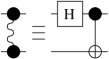
Figure 1. This diagram represents an entangling gate, denoted by $E$. This gate can be locally implemented using a Hadamard gate and a CNOT gate, as shown. A distributed version of the entangling gate is discussed in section 4.

To reduce the complexity of diagrams, we introduce a diagram for an entangling gate, called an $E$ gate, as shown in figure 1. Two qubits are entangled by this $E$ gate. In particular, if the input state is $|{00}\rangle$, the output state will be ${1\over\sqrt{2}}(|{00}\rangle+|{11}\rangle)$.

The entangling gate $E$ can be generalized to an $m$-fold entangling gate, denoted by $E_{m}$, which creates the cat state ${1\over\sqrt{2}}(|{00\ldots 0}\rangle+|{11\ldots 1}\rangle)$ upon the input state $|{00\ldots 0}\rangle$. The $E_{3}$ gate is illustrated in figure 2.

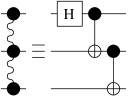
Figure 2. This diagram represents a generalized entangling gate for 3 qubits, denoted by $E_{3}$. It creates the GHZ state if the input is the state $|{000}\rangle$. This gate can be locally implemented by a Hadamard gate and two CNOT gates, as shown.

Finally, figure 3 shows a diagram for the swap gate. Section 4 discusses the distributed implementations of the $E_{m}$ gate and the swap gate.

Figure 3. A swap gate. The discussion of distributed implementation of this gate can be found on section 4.4

2. Distributing Control via a Cat-like State

In this section, we discuss how a cat-like state can distribute control over multiple computers. This is the key idea of the construction of non-local interaction presented in this paper. We will demonstrate this idea using the simplest control gate, i.e., the CNOT gate.

The CNOT gate $\wedge_{1}(X)$ is defined on a two-qubit system as follows: For any control qubit $\alpha|{0}\rangle+\beta|{1}\rangle$ and target bit $|{t}\rangle$,

(2.1) $$\wedge_{1}(X)((\alpha|{0}\rangle+\beta|{1}\rangle)|{t}\rangle) = \alpha|{0}\rangle|{t}\rangle+\beta|{1}\rangle X(|{t}\rangle).$$

We assume that a cat-state ${1\over\sqrt{2}}(|{0\ldots 0}\rangle+|{1\ldots 1}\rangle)$ has already been shared between multiple computers. Then cat-entangler can be used to transform a control qubit and a cat-state into a cat-like state. As a result, equation 2.1 becomes

(2.2) $$\alpha|{00\ldots 0}\rangle|{t}\rangle+\beta|{11\ldots 1}\rangle X(|{t}\rangle),$$

which can be rewritten as

(2.3) $$\wedge_{1}(X)((\alpha|{00\ldots 0}\rangle+\beta|{11\ldots 1}\rangle)|{t}\rangle).$$

Equations 2.2 and 2.3 show that we can use any qubit, shared in the cat-like state, as a control line. For example, the two circuits in figure 4 have an equivalent effect on the target bit, assuming that the state of lines one and two is the cat-like state $\alpha|{00}\rangle+\beta|{11}\rangle$.

Figure 4. Since line one and line two are in the state $|{c}\rangle=\alpha|{00}\rangle+\beta|{11}\rangle$, the target qubit $|{t}\rangle$ can be controlled by either line one or two.

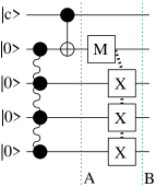
Figure 5. Given a qubit $|{c}\rangle=\alpha|{0}\rangle+\beta|{1}\rangle$ and a generalized GHZ state ${1\over\sqrt{2}}(|{0000}\rangle+\beta|{1111}\rangle)$, created by an entangling gate $E_{4}$, one can create a cat-like state $\alpha|{0000}\rangle+\beta|{1111}\rangle$ with the above circuit.

A cat-entangler is shown in figure 5. The box labeled by $M$ is a standard basis measurement. Since a result of the measurement (represented by a dotted line) is a classical bit, we can distribute and reuse the result to control many $X$-gates at the same time.

Theorem 2.1.

Given a qubit $|{c}\rangle=\alpha|{0}\rangle+\beta|{1}\rangle$ and an $m$-fold cat state ${1\over\sqrt{2}}(|{00\ldots 0_{m}}\rangle+|{11\ldots 1_{m}}\rangle)$, a cat-like state $|{\psi_{c}}\rangle=\alpha|{00\ldots 0_{m}}\rangle+\beta|{11\ldots 1_{m}}\rangle$ can be created by a CNOT gate, local operations (i.e., one measurement and $X$-gates), and classical communication.

Proof: A quantum circuit that creates an $m$-fold cat-like state can be generalized from the circuit shown in figure 5. Assume that an m-fold GHZ state is created by a $E_{m}$ gate.

At point A, after applying the CNOT gate, the state of the circuit is

(2.4) $${1\over\sqrt{2}}(\alpha|{000\dots 0_{m}}\rangle+\alpha|{011\ldots 1_{m}}\rangle+\beta|{110\ldots 0_{m}}\rangle+\beta|{101\ldots 1_{m}}\rangle)$$

After the measurement, the state is either

(2.5a) $$\alpha|{0\underline{0}0\dots 0_{m}}\rangle+\beta|{1\underline{0}1\ldots 1_{m}}\rangle$$

or

(2.5b) $$\alpha|{0\underline{1}1\dots 1_{m}}\rangle+\beta|{1\underline{1}0\ldots 0_{m}}\rangle,$$

where the underlined qubit is the measured qubit.

Assume that the result of measurement is a classical bit $r$. After applying $X$ controlled by the classical bit $r$ (represented by a dotted line on the $X$ gates), the state at point B is

(2.6) $$\alpha|{0\underline{r}0\dots 0_{m}}\rangle+\beta|{1\underline{r}1\ldots 1_{m}}\rangle.$$

Hence, an m-fold cat-like state shared between the qubit $|{c}\rangle$ and other qubits from the cat state (except the measured qubit) is created.

To complete the non-local CNOT operation, the control line must be disentangled and restored. This can be accomplished by a cat-disentangler, as demonstrated in figure 6.

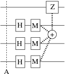
Figure 6. An input state at point $A$, $\alpha|{0000}\rangle+\beta|{1111}\rangle$, is transformed by a cat-disentangler into a state $(\alpha|{0}\rangle+\beta|{1}\rangle)|{r_{2}r_{3}r_{4}}\rangle$, where $r_{k}$ is the result of measurements on line $k$. The phase-flip gate ($Z$-gate) is controlled by the mod 2 sum of the $r_{k}$, written by $\oplus_{k}r_{k}$.

Theorem 2.2.

A state $|{\psi_{c}}\rangle=\alpha|{00\ldots 0_{m}}\rangle+\beta|{11\ldots 1_{m}}\rangle$ can be transformed into a state $\alpha|{0}\rangle+\beta|{1}\rangle)|{r}\rangle$, where $r\in\left\{{0,1,\ldots,2^{m-1}-1}\right\}$ is the result of $m$ $1$-qubit measurements, by a cat-disentangler, which can be generalized from the circuit shown in figure 6.

Proof: Assume the input of the circuit is $|{\psi_{c}}\rangle$. After applying Hadamard transformations, the state of the circuit is

(2.7) $$\alpha|{0}\rangle\sum_{r=0}^{2^{m-1}-1}|{r}\rangle+\beta|{1}\rangle\sum_{r=0}^{2^{m-1}-1}(-1)^{\oplus_{k}r_{k}}|{r}\rangle$$

where the binary representation of $r$ is $r_{1}r_{2}\cdots r_{m-1}$.

After the measurements, the state becomes

(2.8) $$(\alpha|{0}\rangle+(-1)^{\oplus_{k}r_{k}}\beta|{1}\rangle)|{r}\rangle$$

where $r_{i}$ is the result of the measurement on line $i+1$.

To correct the phase, we use the result of the computation $\oplus_{k}r_{k}$ to control the $Z$ gate applied to the first line. Hence, the state at the end of the circuit is $(\alpha|{0}\rangle+\beta|{1}\rangle)|{r}\rangle$.

By considering the circuit in figure 6, the first line can be switched with another line. Therefore, the control state can be restored to any qubit involved in the cat-like state. Furthermore, we can leave more qubits to be untouched, which means we do not apply Hadamard and measurement on one or more qubits. As a result, the remaining qubits form a smaller cat-like state.

2.1. Constructing a Teleportation Circuit

A teleportation circuit can be considered as a composition of the cat-entangler and cat-disentangler as shown in figure 7.

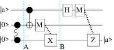
Figure 7. This figure shows a construction of a teleportation circuit using the cat-entangler and cat-disentangler. An unknown quantum state $|{a}\rangle$ is teleported from the first line to the third line.

If the cat-entangler is applied, then the state of qubits $1$ and $3$ is in the cat-like state $\alpha|{00}\rangle+\beta|{11}\rangle$. We next apply the cat-disentangler. However, the unknown qubit $|{a}\rangle$ is restored on line $3$, not on line $1$.

After carefully considering the teleportation circuit, the group of operations applied on the first two qubits after the entangling gate, is actually the Bell basis transformation followed by standard basis measurement. These operations are equivalent to a complete Bell measurement. Furthermore, the result of the measurement is used to control the $X$ and $Z$ gates, as in the teleportation circuit described in [3].

3. Constructing Non-local Control Gates

In this section, we begin by discussing the construction of a non-local CNOT gate. Then we show how to construct efficient distributed control gates in different situations. We assume that we have distributed entangling gates, which create and share a cat state among multiple computers. Construction of distributed entangling gates is described in section 4.

3.1. Constructing a Non-local CNOT Gate

By observing that a control line can be distributed by a cat-like state, a non-local CNOT gate can be implemented as shown in figure 8.

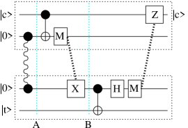
Figure 8. After applying the cat-entangler, the state of the control line and the third line becomes a cat-like state $\alpha|{00}\rangle+\beta|{11}\rangle$. Instead of using the control line (the first line) directly, line $3$ can be used to control line 4. Then we apply a cat-disentangler to restore the control qubit. Each computer boundary is indicated by a tightly dotted box.

Theorem 3.1.

Given a control line $|{c}\rangle=\alpha|{0}\rangle+\beta|{1}\rangle$ and an entangled pair ${{1\over\sqrt{2}}(|{00}\rangle+|{11}\rangle)}$ created by an entangling gate, a non-local CNOT gate can be implemented from the cat-entangler and cat-disentangler, as shown in the figure 8.

Proof: After applying the cat-entangler, the state at point $B$ is

(3.1) $$(\alpha|{0r0}\rangle+\beta|{1r1}\rangle)|{t}\rangle,$$

where $r$ denotes the result of the measurement.

Since line 1 and line 3 are in a cat-like state $\alpha|{00}\rangle+\beta|{11}\rangle$. We can use either line 1 or line 3 to control the $X$ gate. In this case, we use line 3, which is on the local machine.

Because the control line does not change after applying CNOT, the state of line 1 and line 3 remains in a cat-like state. Therefore after applying the cat-disentangler, the control qubit is restored to line 1. Hence, we have completed a non-local CNOT operation.

This circuit is proven to be the optimal implementation by [1, 4], i.e. one ebit and two cbits are necessary and sufficient for implementing a non-local CNOT gate. Furthermore, the cat-entangler and cat-disentangler can be applied to create a $\wedge_{1}(U)$. In many cases, we have an efficient implementation of $\wedge_{1}(U)$.

3.2. Constructing of Small Non-local Control Gates

In this section, we assume that a unitary transformation $U$ is small enough to implement on one computer, but that the control line is on a different computer. Moreover, the transformation $U$ is composed of a number of basic gates, i.e, $U=U_{1}\cdot U_{2}\cdots U_{k}$, for some integer $k$.

After a cat-entangler creates a cat-like state, this establish distributed control between two computers. Since the control line can be reused, only one cat-entangler is needed. Therefore, one ebit and two cbits are needed to implement this type of non-local $\wedge_{1}(U)$ gate. This idea is demonstrated in figure 9, where $U=U_{1}\cdot U_{2}\cdot CNOT$.

Because the control line is reused, the cost of implementing the $\wedge_{1}(U_{i})$ gates can be shared among the basic gates. In other words, each non-local $\wedge_{1}(U_{i})$ can be implemented using only ${1\over{k}}$ ebits and $2\over k$ cbits, asymptotically.

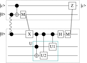
Figure 9. Assume $U=U_{1}\cdot U_{2}\cdot CNOT$. Then $\wedge_{1}(U)=\wedge_{1}(U_{1})\cdot\wedge_{1}(U_{2})\cdot\wedge_{1}(CNOT)$ can be distributed as shown. The control line needs to be distributed only once, because it can be reused. This implementation allows the cost of distributing the control qubit to be shared among the elementary gates.

3.3. Constructing Large Non-local Control-U Gates

In this section, we assume that a unitary transformation $U$ is too big to implement on one computer. Therefore, $U$ has to be decomposed into a number of smaller transformations, where each transformation can be implemented on one computer. In this setting, there are two scenarios to consider.

In the first scenario, we assume that there are no shared qubits between the components of $U$, i.e. $U$ is decomposed into smaller transformations, where each transformation is applied to different qubits. For example, assume $U$ is a unitary transformation for a 7-qubit system, and $U=U_{1}\cdot U_{2}\cdot U_{3}$, where $U_{1}$ is a unitary transformation acting on qubits 1 and 2, $U_{2}$ is a unitary transformation acting on qubits 3, 4, and 5, and $U_{3}$ is a unitary transformation acting on qubits 6 and 7. In this case, not only the cat-like state can be used to distribute a control line among three computers, but $\wedge_{1}(U)$ can also be executed in parallel, as demonstrated in figure 10.

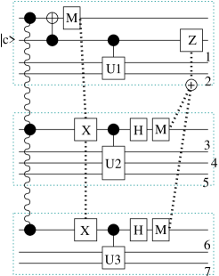
Figure 10. In this case, the transformation $U$ can be decomposed into a set of small transformations. The cat-like state allows the control to be distributed among multiple computers, and also allows each computer to execute in parallel.

In the second scenario, there are shared qubits between these transformations. For example, assume a transformation $U$ is a transformation on a 3-qubit system, and $U=U_{1}\cdot U_{2}\cdot U_{3}\cdot U_{4}$, where $U_{1},U_{4}$ acts on qubit 1 and 2 and $U_{2},U_{3}$ acts on qubit 2 and 3.

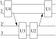
Figure 11. $U$ can be decomposed into a set of smaller transformations that can be implemented on one computer. However, they share qubit number $2$. A distributed version of this case can be implemented by transporting or teleporting qubit number $2$ back and forth between the top and the bottom machine. Line $2$ becomes line $2^{\prime}$ in the bottom computer.

In this case, the shared qubits can be physically transported or teleported from one computer to another. However, sending this shared qubit introduces a communication overhead, which is not present in a non-distributed implementation of $\wedge_{1}(U)$.

3.4. Constructing a $\wedge_{m}(U)$ Gate

A non-local $\wedge_{m}(U)$ can simply be implemented by using $m$ cat-like pairs to distribute $m$ control qubits to one machine, and then to implement $\wedge_{m}(U)$ locally, as suggested in [1]. Figure 12 shows an instance of $\wedge_{2}(U)$.

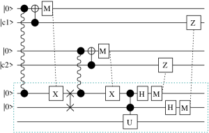
Figure 12. Both control lines $|{c_{1}}\rangle$ and $|{c_{2}}\rangle$ are distributed via two cat-like states to the bottom machine so that $\wedge_{2}(U)$ can be implemented locally. The swap gate moves the control line from the channel qubit and resets it to $|{0}\rangle$, so that the channel qubit can be reused.

However, this requires the computer to have enough qubits to implement $\wedge_{m}(U)$ locally. Therefore, the number of non-local control lines is limited by the number of qubits available on one computer.

Figure 13. In this case, $m=6$ and $n=2$. The $\wedge_{4}(X)$ gate is simulated by two $\wedge_{2}$ gates and two $\wedge_{3}$ gates as shown.

Barenco et al show that the $\wedge_{m-2}(X)$ gate can be linearly simulated on $m$-qubit system [5]. For example, for any $m\geq 5$, $2\leq n\leq m-3$, a $\wedge_{m-2}(X)$ gate can be implemented as two $\wedge_{n}(X)$ gates and two $\wedge_{m-n-1}(X)$ gates on an $m$-qubit system. An implementation for the case of $m=6$ and $n=2$ is shown in figure 13.

This technique can be used to break down a large $\wedge_{m}(U)$ gate into a sequence of smaller gates. After thus making the number of control lines small enough, we can distribute these control lines to one machine, and implement each gate locally.

A distributed implementation of figure 13 is demonstrated in figure 14. We group lines 1, 2, and 5 together on the top machine. Then we distribute line 5 to line 5’ and then use it to perform a control operation with lines 3 and 4 applied to line 6 in the bottom machine.

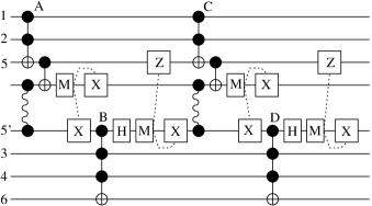
Figure 14. This circuit presents a distributed version of $\wedge_{4}(X)$, where $m=6$ and $n=2$. Line 5 becomes line 5’ on the bottom machine.

4. Establishing and Refreshing an Entangled Pair

Before any non-local CNOT and teleportation operations are performed, an entangled pair must be established between channel computers. Moreover, after the operation is finished, the channel qubits must be reset to refresh the pair. We discuss establishing and refreshing procedure in the next section via the construction of entangling gates.

4.1. Constructing the $E_{2}$ Gate

Because establishing entanglement can not be accomplished by any local operations, channel qubits must be on one machine. The simplest way to establish an entangled pair is described as follow:

To establish an ebit between a remote and a local computers, the remote computer sends a channel qubit to the local machine. Then, the local machine entangles the remote channel qubit with one of the local channel qubits. Then one qubit of the pair is sent back to the remote machine. This process establishes one ebit by sending two qubits, one in each direction.

If we allow each machine to have two channel qubits, then two ebits can be established by sending two qubits. To do so, each computer entangles its own channel qubits, then exchanges one qubit of the pair with the other computer, as demonstrated in figure 15. As a result, one ebit is established with the cost of sending one qubit, asymptotically. To refresh the entanglement, the procedure is simply repeated. However, the channel qubits must be reset to state $|{0}\rangle$ before they can be re-entangled.

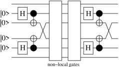
Figure 15. Assuming each machine holds a pair of channel qubits. Each machine entangles its channel pair, and then exchanges one qubit of the pair with another machine.

Channel qubits need to be in the state $|{0}\rangle$ before being entangled. Therefore the channel qubits must be reset to the state $|{0}\rangle$ before the entangled pair can be refreshed. Because the measurement result reveals the current state of the measured qubit, we can use the measurement result to control the $X$-gate to set the channel qubit to $|{0}\rangle$, as shown in figure 16.

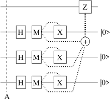
Figure 16. This figure demonstrates how the channel qubits can be reset to $|{0}\rangle$ by considering the result of the measurement. Assume the input state at point A is $\alpha|{0000}\rangle+\beta|{1111}\rangle$. The output of the circuit is the state $(\alpha|{0}\rangle+\beta|{1}\rangle)|{000}\rangle$.

4.2. Constructing the $E_{m}$ Gate

A non-distributed version of $E_{m}$ gate can be linearly implemented using a Hadamard gate, and a sequence of CNOT gates as shown in figure 2 (for three qubits case.) However, it takes $O(m)$ steps to create an m-fold GHZ state. An efficient way of implementing a non-distributed version of an $E_{m}$ gate is shown in figure 17. This implementation utilizes a binary tree idea to reduce the number of steps from $O(m)$ to $O(\log m)$.

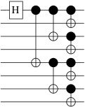
Figure 17. This figure represent an efficient implementation of $G_{8}$, using a Hadamard gate and 7 CNOT gates. A generalized GHZ state can be created after applying $O(\log m)$ gates. However, this implementation requires more channel qubits.

A distributed version of $E_{m}$ gate can be implemented by using non-local CNOT gates. In this process, we exchange $m-1$ ebits with the $m$-fold cat state by replacing CNOT gates with non-local CNOT gates.

In the linear implementation of $E_{m}$, each computer requires at least two channel qubits to establish entanglement with its neighbors. This number is fixed regardless of the number of computers involved.

On the contrary, in the binary implementation, the number of channel qubits on each computer increases with respect to $m$. In fact, the number of channel qubits required is $O(\log m)$. This is true because the first computer has to simultaneously establish $O(\log m)$ entangled pairs with others computers, as shown in figure 17, before an $m$-fold cat state is created. However, the trade off is justified because the number of steps required to establish the $m$-fold cat state is reduced from $O(m)$ to $O(\log m)$.

4.3. Re-constructing a Teleportation Circuit

In the implementation of a non-local CNOT gate, measurements are performed on both channel qubits. Therefore, the channel qubits can be reset by considering the measurement results. In the teleportation circuit, the remote channel qubit is not measured. Moreover, it holds the unknown state which is teleported by the circuit. Pati and Braunstein show in [9] that an unknown qubit can not be deleted. To solve this problem, we can swap the remote channel qubit with $|{0}\rangle$ held by another qubit in the register on the same machine. By swapping, the unknown qubit is preserved and the channel qubit is reset. The construction of the teleportation circuit, with channel qubits reset, is shown in figure 18.

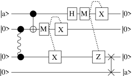
Figure 18. The remote channel qubit can be reset by swapping with a empty qubit ($|{0}\rangle$). In addition, after teleportation, the original qubit is reset to $|{0}\rangle$ state.

One remaining question is how many $|{0}\rangle^{\prime}s$ (or empty qubits) are needed to support the teleportation protocol. We observe that, after teleportation, the original unknown qubit on the source machine is reset to state $|{0}\rangle$. Therefore, we can use this qubit as an empty qubit in the next inbound teleportation. However, the required number of empty qubits still depends on how many qubits are teleported into the machine before another qubit is teleported out. In other words, we can consider the $|{0}\rangle$ qubit as an empty space. To teleport a qubit in, we need an empty space to receive the qubit. The more qubits teleported into the machine, the more spaces needed.

4.4. Constructing a Distributed Swap Gate

A distributed swap gate can be implemented by using two teleportations to exchange two qubits. If each machine has two channel qubits involved in a swapping operation, we do not need any empty qubits in the registers. The channel qubit becomes a swapping buffer, because the first teleportation creates an empty qubit for the second teleportation to use. However, if we have only one channel qubit in a swapping operation, one empty qubit is needed for a swapping buffer.

In [4], Collins, Linden, and Popescu show that an optimal non-local swap gate requires two ebits and two cbits in each direction. Therefore, implementing a swap gate by two teleportations is an optimal implementation.

5. Distributed Fourier Transform

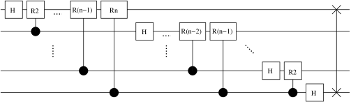
Figure 19. The Fourier transformation is a sequence of Hadamard and control-$R_{k}$ gates. At the end, a swapping gate is used to reset the order of the qubits.

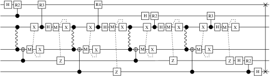
Figure 20. By applying non-local control $R_{k}$ gates, we construct a distributed Fourier transformation. This figure shows the distributed Fourier transformation for 4 qubits which is implemented on two machines. The swap gate can be implemented by teleporting qubits back and forth between two computers.

The quantum Fourier transform is a unitary transformation defined on basis states as follows,

(5.1) $$|{j}\rangle\rightarrow{1\over{\sqrt{2^{n}}}}\sum_{k=0}^{2^{n}-1}e^{2\pi\imath jk/2^{n}}|{k}\rangle,$$

where $n$ is the number of qubits. See [2, 10] for more details.

Shor presents the quantum Fourier transformation in [2] as a routine used in the factoring algorithm. Later on, it becomes a standard routine used in many quantum algorithms, such as phase estimation, and the hidden subgroup algorithms. An efficient circuit for the quantum Fourier transformation, found in [10], is shown in figure 19. The gate $R_{k}$ is defined as follows,

(5.4) $$R_{k}=\left(\begin{array}[]{cc}{1}&{0}\\ {0}&{e^{2\pi\imath/2^{k}}}\end{array}\right),$$

where $k\in\left\{{2,3,\ldots}\right\}$.

We use the construction of $\wedge_{1}(U)$ to implement a distributed version of the Fourier transformation. The swap gate can be implemented by teleporting qubits back and forth between two computers.

The communication resources needed depend on how many non-local control gates have to be implemented. Assume that we implement the Fourier transformation on $m$ computers, and each computer has $k$ qubits, not including the channel qubits. Let $n=mk$. Therefore, there are $(n-1)n/2$ control gates to implement. Hence, for each computer, there are $(k-1)k/2$ local control gates. The number of local control gates is $m(k-1)k/2=(n/m-1)n/2$. The number of non-local control gates is $(n-1)n/2-(n/m-1)n/2$ gates. Hence, the communication resources are $O(n^{2})$.

An implementation of the distributed Fourier transformation of $4$ qubits is shown in figure 20

6. Conclusion

The teleportation circuit and the non-local CNOT gate can be implemented using two primitive operations, cat-entangler and cat-disentangler. These two primitive operations work on the idea that a cat-like state can be used to distribute a control line. This principle is extended to construct non-local operations efficiently in many cases.

For example, the communication cost can be shared among elementary gates because a control line can be reused after being distributed via cat-like state. Moreover, the cat-like state allows parallel implementation of some control gates.

Before using a non-local operation, an entanglement has to be established. Moreover, it has to be refreshed after being used. Fortunately, by looking at the measurement results, we can reset channel qubits, and re-establish entanglement. This procedure works well with non-local CNOT gates. To reset channel qubits in the teleportation operation, the channel qubits have to be swapped with empty qubits ($|{0}\rangle$).

In general, if we can break down a unitary transformation into a sequence of CNOT gates and one-qubit gates, a distributed version of the unitary transformation can be simply implemented by replacing CNOT gates with non-local CNOT gates. Therefore, the communication overhead is dependent on the number of non-local CNOT gates needed to be implemented. With help from teleportation to move qubits back and forth between computers, better distributed implementation can be accomplished.

References

- [1] J. Eisert, K. Jacobs, P. Papadopoulos, and M.B. Plenio, Phys. Rev. A, 62, 052317-1 (2000). quant-ph/0005101.
- [2] Peter W. Shor, quant-ph/9508027 (1995).
- [3] Charles H. Bennett, Gilles Brassard, Claude Crépeau, Richard Jozsa, Asher Peres, and William K. Wootters, Phys. Rev. Lett. 70, 1895 (1993).
- [4] Daniel Collins, Noah Linden, and Sandu Popescu, Phys. Rev. A, 64, 032302 (2001). quant-ph/0005102.
- [5] Adriano Barenco, Charles H. Bennett, Richard Cleve, David P. DiVincenzo, Norman Margolus, Perter Shor, Tycho Sleator, John A. Smolin, and Harald Weinfurter, Phys. Rev. A, 52, 3457 (1995). quant-ph/9503016.
- [6] K. Brennen, Daegene Song, and Carl J. Williams, quant-ph/0301012 (2003).
- [7] M. Zekowski, A. Zeilinger, M.A. Horne and A.K. Ekert, Phys. Rev. Lett, 71, 4287 (1993); S. Bose, V. Vedral and P.L. Knight, Phys. Rev. A, 57, 822 (1998).
- [8] S. Bose, V. Vedral, and P.L. Knight, Phys. Rev. A, vol 57 822 (1997); Lucien Hardy and David D. Song, Phys. Rev. A, vol 62, 052315 (2000).
- [9] Arun K. Pati and Samuel L. Braunstein, quant-ph/9911090 v2 (2000).
- [10] M. A. Nielsen and I. L. Chuang, “Quantum Computation and Quantum Information”, Cambridge press, 2000.