Quantum Phase Space in Relativistic Theory:
the Case of Charge-Invariant Observables

Abstract

Mathematical method of quantum phase space is very useful in physical applications like quantum optics and non-relativistic quantum mechanics. However, attempts to generalize it for the relativistic case lead to some difficulties. One of problems is band structure of energy spectrum for a relativistic particle. This corresponds to an internal degree of freedom, so-called charge variable. In physical problems we often deal with such of dynamical variables that do not depend on this degree of freedom. These are position, momentum, and any combination of them. Restricting our consideration to this kind of observables we propose the relativistic Weyl–Wigner–Moyal formalism that contains some surprising differences from its non-relativistic counterpart.

This paper is devoted to the phase space formalism that is specific representation of quantum mechanics. This representation is very close to classical mechanics and its basic idea is a description of quantum observables by means of functions in phase space (symbols) instead of operators in the Hilbert space of states.

The first idea about this representation has been proposed in the early days of quantum mechanics in the well-known Weyl work [1]. Let us put the operator $\hat{A}$, which acts in the Hilbert space of states of a quantum system, into correspondence to a function on the phase space (symbol) $A\left(p,q\right)$ according with the following rule

$$\hat{A}=\int\limits_{-\infty}^{+\infty}A\left(p,q\right)\hat{W}\left(p,q\right)dpdq,$$ (1)

where $\hat{W}\left(p,q\right)$ is an operator generalization of $\delta$-function that is called operator of quasiprobability density. This operator is defined as Fourier image of operator exponent (operator of representation of the Heisenberg-Weyl group)

$$\hat{W}\left(p,q\right)=\frac{1}{2\pi\hbar}\int\limits_{-\infty}^{+\infty}\exp\left\{\frac{i}{\hbar}\left[Q\left(p-\hat{p}\right)-P\left(q-\hat{q}\right)\right]\right\}dQdP.$$ (2)

Nowadays, this transformation is known as Weyl transform.

In table 1 one can find correspondences among some constructions in classical mechanics and in the Hilbert space and phase space representations of quantum mechanics. First of all, it is related to two binar operations, namely, usual product and bracket. In classical mechanics there exist conventional commutative multiplication of two functions and Poisson bracket. It is well known that corresponding operations in the Hilbert space representation of quantum mechanics are non-commutative product of two observables and commutator. In the phase space representation of quantum mechanics we deal with so-called star product and Moyal bracket.

Table 1: Some constructions in classical mechanics and in quantum mechanics (Hilbert space and phase space representations) are shown. First line corresponds to the usual product of two observables. Brackets (Poisson, commutator, Moyal) are shown in the second line. Evolution equations in Heisenberg and Schrödinger representations are presented in third and fourth lines respectively. In the fifth line one can see expressions for mean value of an observable. Expressions for a pure state are presented in the sixth line.

Classical mechanics	Quantum mechanics (Hilbert space)	Quantum mechanics (phase space)
$A\left(p,q\right)B\left(p,q\right)$	$\hat{A}\hat{B}$	$\scriptstyle{A\left(p,q\right)\star B\left(p,q\right)},$ $\scriptstyle{\star=\exp\left\{\frac{i\hbar}{2}\left(\overleftarrow{\partial_{q}}\overrightarrow{\partial_{p}}-\overleftarrow{\partial_{p}}\overrightarrow{\partial_{q}}\right)\right\}}$
$\begin{array}[]{l}\left\{A(p,q),B(p,q)\right\}_{P}\\ \scriptstyle{=A(p,q)\left(\overleftarrow{\partial_{q}}\overrightarrow{\partial_{p}}-\overleftarrow{\partial_{p}}\overrightarrow{\partial_{q}}\right)B(p,q)}\end{array}$	$\left[\hat{A},\hat{B}\right]=\hat{A}\hat{B}-\hat{B}\hat{A}$	$\begin{array}[]{l}\left\{A(p,q),B(p,q)\right\}_{M}\\ \scriptstyle{=\frac{1}{i\hbar}\left(A(p,q)\star B(p,q)-B(p,q)\star A(p,q)\right)}\\ \scriptstyle{=\frac{2}{\hbar}A(p,q)\sin\left\{\frac{\hbar}{2}\left(\overleftarrow{\partial_{q}}\overrightarrow{\partial_{p}}-\overleftarrow{\partial_{p}}\overrightarrow{\partial_{q}}\right)\right\}B(p,q)}\end{array}$
$\partial_{t}A=\left\{A,H\right\}_{P}$	$\partial_{t}\hat{A}=\frac{1}{i\hbar}\left[\hat{A},\hat{H}\right]$	$\partial_{t}A=\left\{A,H\right\}_{M}$
$\partial_{t}\rho=\left\{H,\rho\right\}_{P}$	$\partial_{t}\hat{\rho}=\frac{1}{i\hbar}\left[\hat{H},\hat{\rho}\right]$	$\partial_{t}W=\left\{H,W\right\}_{M}$
$\scriptstyle{\bar{A}=\int\limits_{-\infty}^{+\infty}A\left(p,q\right)\rho\left(p,q\right)dpdq}$	$\bar{A}=\mathop{\mathrm{Tr}}\nolimits\left(\hat{A}\hat{\rho}\right)$	$\scriptstyle{\bar{A}=\int\limits_{-\infty}^{+\infty}A\left(p,q\right)W\left(p,q\right)dpdq}$
$\begin{array}[]{l}\scriptstyle{\rho\left(p,q\right)=\delta\left(p-p(t)\right)\delta\left(q-q(t)\right)}\\ {}\scriptstyle\end{array}$	$\hat{\rho}=\left|\psi\right\rangle\left\langle\psi\right|$	$\begin{array}[]{l}\scriptstyle{W\left(p,q\right)}\\ \scriptstyle{=\frac{1}{{2\pi\hbar}}\int\limits_{-\infty}^{+\infty}{\psi^{*}\left({p+\frac{P}{2}}\right)\psi\left({p-\frac{P}{2}}\right)e^{-\frac{i}{\hbar}Pq}dP}}\end{array}$

One can see a very important property: when $\hbar\rightarrow 0$, quantum mechanics in the phase space transforms to classical mechanics.

Now, it is possible to write down quantum counterparts for the evolution equations (Hamilton or Liouville), expressions for expected values of observables, and distribution function for a pure state. In quantum mechanics this function has been presented firstly by Wigner in 1932 [2], and nowadays is well-known as Wigner function.

This formalism is very useful in a lot of branches of modern physics, e.g. in quantum optics (see for an example [3].) The fact that Wigner function does not satisfy Kolmogorov axiomatic for probability has helped us to better understand the nature of quantum non-locality [4], [5].

However, generalization of this formalism to the relativistic case meets some problems. A very interesting feature is the fact that Weyl transform is not Lorentz invariant in an explicit form. We do not consider this question in the paper. Some consideration of it and references one can find in [6], [7]. Here, we concentrate our attention on another problem, that is absence of a well-defined position operator in relativistic case.

Consider the simplest example, a scalar charged particle in a constant magnetic field. This system is described by the Klein–Gordon equation

$$-\hbar^{2}\partial_{t}^{2}\Psi=\left(c^{2}\left(\hat{p}-eA\left(q\right)\right)^{2}+m^{2}c^{4}\right)\Psi.$$ (3)

This is well-known that energy spectrum of this equations is subdivided in two bands: lower and upper (see Fig. 1)

$$E\left(n,\pm\right)=\pm mc^{2}\sqrt{1+\frac{2}{mc^{2}}e\left(n\right)},$$ (4)

where $e\left(n\right)$ is the spectrum of a non-relativistic particle. Moreover, according with modern notions about the field theory, one supposes that lower band is occupied by particles (so-called Dirak Sea.)

Figure 1: Energy spectrum of a relativistic particle.

The Klein–Gordon equation is a second-order equation in time. One can rewrite it in accordance with the Feshbach–Villars formalism [8] as a system of two first-order equations. To achieve this one should provide changing variables

$$\Psi=\frac{1}{\sqrt{2}}\left(\varphi+\chi\right), i\hbar\partial_{t}\Psi=\frac{mc^{2}}{\sqrt{2}}\left(\varphi-\chi\right).$$ (5)

As a result we can write down the Klein–Gordon equation in the form of the Schrödinger equation

$$i\hbar\partial_{t}\psi=\hat{H}\psi,$$ (6)

with two-component wave function $\psi=\left(\begin{array}[]{c}\varphi\\ \chi\end{array}\right)$ and Hamiltonian $\hat{H}=\left(\tau_{3}+i\tau_{2}\right)e\left(\hat{n}\right)+\tau_{3}mc^{2}$. In the last equation $e\left(\hat{n}\right)$ is non-relativistic Hamiltonian, and $\tau_{i}$ are the Pauli matrices. In fact, they present a specific internal degree of freedom, so-called charge variable.

The point is that eigenfunctions of position and momentum operators belong to both bands. Hence, the question about measurement of position and momentum in the relativistic case is not so trivial.

If one has an aim to construct the phase space formalism for a relativistic particle, the charge variable should be taken into account as an independent degree of freedom, and $\tau_{i}$ have to be considered as a specific part of the phase space. Such a kind of formalism would be very useful. However, we will consider a simpler case.

Let us restrict our attention only to such observables that commute with all matrices $\tau_{i}$

$$\left[\hat{A},\tau_{i}\right]=0, i=1,2,3.$$ for (7)

In fact, this means that these observables are operator functions of position and momentum and do not depend on $\tau_{i}$

$$\hat{A}=F\left(\hat{p},\hat{q}\right).$$ (8)

We call elements of corresponding subalgebra of the dynamical algebra as charge-invariant observables. Indeed, all these operators are invariant relatively to unitary transformations (or, to be more precise, generalized unitary transformations [8]) in charge subspace of the Hilbert space. A lot of important observables belong to the subalgebra of charge-invariant observables. These are position, momentum, second moments, etc. However, it is worth noting that Hamiltonian and current do not belong to this subalgebra. Hence, one cannot use formalism presented here for those ones.

Using the phase space formalism, one can provide analysis for such a subalgebra of dynamical algebra. An interesting feature of these observables is the fact that even $[A]$ and odd $\{A\}$ parts of corresponding operators (diagonal and not diagonal components of matrices $2\times 2$ in the energy representation, see [8]) are not independent. In [6], [7], one can find a proof of the following constraint for them (in the energy representation)

$$\{A\}_{nm}=\frac{{E(m)-E(n)}}{{E(m)+E(n)}}\tau_{1}[A]_{nm}.$$ (9)

Another very important property of charge-invariant observables is the fact that it is possible for them to present usual (scalar, not matrix-valued) Wigner function with conventional rule for the calculation of mean values

$$\overline{A}=\int\limits_{-\infty}^{+\infty}A(p,q)W(p,q)dpdq.$$ (10)

Nevertheless, there are very important differences from the non-relativistic case. First of all, this object is a sum of four components

$$W(p,q)=\sum_{\alpha=\pm 1}\left(W_{[\alpha]}(p,q)+W_{\{\alpha\}}(p,q)\right).$$ (11)

Namely, these are two even components, which correspond to particle and antiparticle

$$W_{[\pm]}(p,q)=\!\sum_{n,m=0}^{\infty}{\varepsilon(m,n)}W_{nm}(p,q)C_{m;}^{*}{}_{\pm}C_{n;}{}^{\pm},$$ (12)

and two odd (non-physical) components, which correspond to the interference between particle and antiparticle

$$W_{\{\pm\}}(p,q)=\!\sum_{n,m=0}^{\infty}{\chi(m,n)}W_{nm}(p,q)C_{m;}^{*}{}_{\pm}C_{n;}{}^{\mp}.$$ (13)

In equations (12) and (13) $C_{n;}{}^{\pm}$ is a wave function in the energy representation, $W_{nm}(p,q)$ is a Hermitian generalization of the Wigner function (see [7], [9]), functions

$$\varepsilon\left(n,m\right)=\frac{{E\left(n\right)+E\left(m\right)}}{{2\sqrt{E\left(n\right)E\left(m\right)}}}$$ (14)

and

$$\chi\left(n,m\right)=\frac{{E\left(n\right)-E\left(m\right)}}{{2\sqrt{E\left(n\right)E\left(m\right)}}}$$ (15)

are so-called $\varepsilon$- and $\chi$-factors.

One can find evolution equations (quantum Liouville equation) for each component separately

$$\partial_{t}W_{[\pm]}(p,q,t)=\pm\left\{E(p,q),W_{[\pm]}(p,q,t)\right\}_{M},$$ (16)

$$\partial_{t}W_{\{\pm\}}(p,q,t)=\mp\left[E(p,q),W_{\{\pm\}}(p,q,t)\right]_{M},$$ (17)

where

$$E(p,q)=\sqrt[\star]{m^{2}c^{4}+c^{2}\left(p-eA\left(q\right)\right)^{2}}$$ (18)

is the effective Hamiltonian. Here one has two surprising features as well.

First of all, the symbol of the Hamiltonian is defined by means of square root in a sense of star product. This means that Weyl symbol of the Hamiltonian differs from the Hamilton function in classical mechanics. In non-relativistic mechanics they coincide.

Second, the evolution equation for the odd components is formulated using “anti-Moyal” bracket, which is counterpart of the anti-commutator. This means that evolution of odd part is a non-unitary operation.

Moreover, there are once more, the most important property. Definition of even component include a very important multiplier, $\varepsilon$-factor (14). It is absent in the non-relativistic theory. Consider its properties more closely:

1. $\varepsilon(n,m)=\varepsilon(m,n)$.

2. $\varepsilon(n,n)=1$.

3. $\varepsilon(n,m)>1$, if $n\neq m$.

This is very similar to the case, when one considers an arbitrary system in an environment. For the Wigner function in this case one can write down the following expression

$$W(p,q)=\sum\limits_{n=0}^{\infty}W_{nn}(p,q)\left|C_{n}\right|^{2}+\sum\limits_{n\neq m}a(m,n)W_{nm}(p,q)C_{m}^{*}C_{n}.$$ (19)

However, non-diagonal components of $a(m,n)$ (counterpart of $\varepsilon$-factor) are always smaller than $1$. Therefore, in the relativistic case, influence of vacuum is inverted to the decoherence process. This means that relativistic system has more quantum non-local properties than its non-relativistic counterpart.

It is possible to consider this question from the more formal point of view. It is well-known that not every normalized function can be regarded as Wigner function presenting a real quantum physical state [10]. In the non-relativistic case there exists so-called quantization condition that selects Wigner functions from set of functions on the phase space. In our case this condition can be presented in the following way (for a free particle).

Theorem 1

For the functions $W_{[\pm]}\left(p,q\right)$ and $W_{\{\pm\}}\left(p,q\right)$ to be even and odd components of the Wigner function for charge-invariant observables, it is necessary and sufficient that all constrains hold true (see [6]) and the following conditions are satisfied:

$$\frac{{\partial^{2}}}{{\partial p_{1}\partial p_{2}}}\ln\int\limits_{-\infty}^{+\infty}W_{[\pm]}\left(\frac{1}{2}(p_{1}+p_{2}),q\right)\exp\left(\frac{i}{\hbar}(p_{1}-p_{2})q\right)dq$$

$$=-\frac{c^{4}p_{1}p_{2}}{E(p_{1})E(p_{2})(E(p_{1})+E(p_{2}))^{2}},$$ (20)

$$\frac{{\partial^{2}}}{{\partial p_{1}\partial p_{2}}}\ln\int\limits_{-\infty}^{+\infty}W_{\{\pm\}}\left(\frac{1}{2}(p_{1}+p_{2}),q\right)\exp\left(\frac{i}{\hbar}(p_{1}-p_{2})q\right)dq$$

$$=-\frac{c^{4}p_{1}p_{2}}{E(p_{1})E(p_{2})(E(p_{1})-E(p_{2}))^{2}}.$$ (21)

A proof of this criterion can be found in [6], and formulation for a more general case in [7].

The main difference from the non-relativistic case is the fact that in the right-hand-side of equation (20) one has an expression that differs from $0$. In the non-relativistic case this is exactly $0$.

Consider a simple example. Figure 2 shows the Wigner function for the coherent state of a free particle [11]. In fact, this is a Gauss distribution for non-strong space localization . However, when localization along position is very strong, additional “vacuum fluctuations” appear. They counteract to the strong localization. This means that coherent state (which is classical in terms of work [5]) manifests a quantum feature.

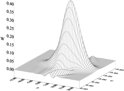
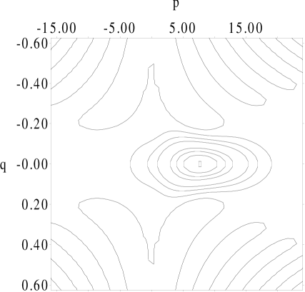
Figure 2: Wigner function and its contours for the coherent state of a free relativistic particle. Position is given in the units of Compton wavelength, momentum is given in $mc$ units.

For a conclusion, we note that quantum quasidistributions of relativistic systems are more different from classical distributions than their non-relativistic counterparts. This means that relativistic systems are more interesting objects for investigation of quantum non-locality and non-classicality.

References

- [1] Weyl H. The theory of groups and quantum mechanics, Dover Publications, Inc., 1931.
- [2] Wigner E.P. On the quantum correction for the thermodynamic equilibrium, Phys. Rev., 1932, V.40, N 5, 749–759.
- [3] Schleich W.P., Quantum optics in phase space, Wiley-VCH, Berlin, 2001.
- [4] Klyshko D.N., Basic quantum mechanical concepts from the operational viewpoint, Physics–Uspekhi, 1998, V.41, N 9, 885–922.
- [5] Richter Th. and Vogel W., Nonclassicality of quantum states: a hierarchy of observable conditions, Phys. Rev. Lett., 2002, V.89, N 28, 283601.
- [6] Lev B.I., Semenov A.A. and Usenko C.V., Pecularities of the Weyl–Wigner–Moyal formalism for scalar charged particle, J. Phys. A: Math. Gen., 2001, V.34, N 20, 4323–4339.
- [7] Lev B.I., Semenov A.A. and Usenko C.V., Scalar charged particle in Weyl–Wigner–Moyal phase space. Constant magnetic field, J. Rus. Las. Res., 2002, V.23, N 4, 347–368. /quant-ph:0112146.
- [8] Feshbach H. and Villars F., Elementary relativisic wave mechanics of spin and spin particles, Rev. Mod. Phys., 1958, V.30, N 1, 24–45.
- [9] Fairlie D.B., The formulation of quantum mechanics in terms of phase space function, Proc. Cambr. Phil. Soc., 1964, V.60, N 3, 581–586.
- [10] Tatarskii V.I. Wigner representation of quantum mechanics, Sov. Physics – Uspekhi, 1983, V.26, N 4, 311.
- [11] Lev B.I., Semenov A.A., Usenko C.V. and Klauder J.R., Relativistic coherent states and charge structure of the coordinate and momentum operators, Phys. Rev. A, 2002, V.66, N 2, 022115.