Feedback Control of Quantum State Reduction

Abstract

Feedback control of quantum mechanical systems must take into account the probabilistic nature of quantum measurement. We formulate quantum feedback control as a problem of stochastic nonlinear control by considering separately a quantum filtering problem and a state feedback control problem for the filter. We explore the use of stochastic Lyapunov techniques for the design of feedback controllers for quantum spin systems and demonstrate the possibility of stabilizing one outcome of a quantum measurement with unit probability.

I Introduction

It is a basic fact of nature that at small scales—at the level of atoms and photons—observations are inherently probabilistic, as described by the theory of quantum mechanics. The traditional formulation of quantum mechanics is very different, however, from the way stochastic processes are modeled. The theory of quantum measurement is notoriously strange in that it does not allow all quantum observables to be measured simultaneously. As such there is yet much progress to be made in the extension of control theory, particularly feedback control, to the quantum domain.

One approach to quantum feedback control is to circumvent measurement entirely by directly feeding back the physical output from the system [1, 2]. In quantum optics, where the system is observed by coupling it to a mode of the electromagnetic field, this corresponds to all-optical feedback. Though this is in many ways an attractive option it is clear that performing a measurement allows greater flexibility in the control design, enabling the use of sophisticated in-loop signal processing and non-optical feedback actuators. Moreover, it is known that some quantum states obtained by measurement are not easily prepared in other ways [3, 4, 5].

We take a different route to quantum feedback control, where measurements play a central role. The key to this approach is that quantum theory, despite its entirely different appearance, is in fact very closely related to Kolmogorov’s classical theory of probability. The essential departure from classical probability is the fact that in quantum theory observables need not commute, which precludes their simultaneous measurement. Kolmogorov’s theory is not equipped to deal with such objects: one can always obtain a joint probability distribution for random variables on a probability space, implying that they can be measured simultaneously. Formalizing these ideas leads naturally to the rich field of noncommutative or quantum probability [6, 7, 8]. Classical probability is obtained as a special case if we consider only commuting observables.

Let us briefly recall the setting of stochastic control theory. The system dynamics and the observation process are usually described by stochastic differential equations of the Itô type. A generic approach to stochastic control [9, 10] separates the problem into two parts. First one constructs a filter which propagates our knowledge of the system state given all observations up to the current time. Then one finds a state feedback law to control the filtering equation. Stochastic control theory has traditionally focused on linear systems, where the optimal (LQG) control problem can be solved explicitly.

A theory of quantum feedback control with measurement can now be developed simply by replacing each ingredient of stochastic control theory by its noncommutative counterpart. In this framework, the system and observations are described by quantum stochastic differential equations. The next step is to obtain quantum filtering equations [11, 12, 13, 14]. Remarkably, the filter is a classical Itô equation due to the fact that the output signal of a laboratory measuring device is a classical stochastic process. The remaining control problem now reduces to a problem of classical stochastic nonlinear control. As in the classical case, the optimal control problem can be solved explicitly for quantum systems with linear dynamics.

The field of quantum stochastic control was pioneered by V. P. Belavkin in a remarkable series of papers [15, 11, 12, 13] in which the quantum counterparts of nonlinear filtering and LQG control were developed. The advantage of the quantum stochastic approach is that the details of quantum probability and measurement are hidden in a quantum filtering equation and we can concentrate our efforts on the classical control problem associated with this equation. Recently the quantum filtering problem was reconsidered by Bouten et al. [14] and quantum optimal control has received some attention in the physics literature [16, 17].

The goal of this paper is twofold. We review the basic ingredients of quantum stochastic control: quantum probability, filtering, and the associated geometric structures. We then demonstrate the use of this framework in a nonlinear control problem. To this end, we study in detail an example directly related to our experimental apparatus [4]. As this is not a linear system, the optimal control problem is intractable and we must resort to methods of stochastic nonlinear control. We use stochastic Lyapunov techniques to design stabilizing controllers, demonstrating the feasibility of such an approach.

We are motivated in studying the quantum control problem by recent developments in experimental quantum optics [4, 18, 19, 20]. Technology has now matured to the point that state-of-the-art experiments can monitor and manipulate atomic and optical systems in real time at the quantum limit; i.e. the sources of extraneous noise are sufficiently suppressed that essentially all the noise is fundamental in nature. The experimental implementation of quantum control systems is thus within reach of current experiments, with important applications in e.g. precision metrology [20, 21, 22, 23] and quantum computing [24, 25]. Further development of quantum control theory is an essential step in this direction.

This paper is organized as follows: in section II we give an introduction to quantum probability and sketch a simple derivation of quantum filtering equations. We also introduce the particular physical system that we study in the remainder of the paper. In section III we study the dynamical behavior of the filtering equation and the underlying geometric structures. Finally, section IV is devoted to the design of stabilizing controllers using stochastic Lyapunov methods.

II Quantum probability and filtering

The purpose of this section is to clarify the connections between quantum mechanics and classical probability theory. The emphasis is not on rigor as we aim for a brief but broad overview; we refer to the references for a complete treatment.

II-A Finite-dimensional quantum probability

We begin by reviewing some of the traditional elements of quantum mechanics (e.g. [26]) with a probabilistic flavor.

An observable of a finite-dimensional quantum system is represented by a self-adjoint linear operator $X=X^{*}$ on some underlying finite-dimensional complex Hilbert space $\mathcal{H}$ ($*$ denotes Hermitian conjugation). Every self-adjoint operator has a spectral decomposition

$$X=\sum_{i}\lambda_{i}P_{i},~{}~{}~{}~{}~{}~{}~{}\lambda_{i}\in\mathbb{R},~{}~{}P_{i}=P_{i}^{2}=P_{i}^{*}$$ (1)

where $\lambda_{i}$ are the eigenvalues of $X$ and $P_{i}$ are projectors onto orthogonal eigenspaces in $\mathcal{H}$ such that $\sum_{i}P_{i}={\rm Id}_{\mathcal{H}}$.

If we were to measure $X$ we would obtain one of the values $\lambda_{i}$ as the measurement outcome. The $P_{i}$ represent the events that can be measured. To complete the picture we still need a probability measure. This is provided by the density operator $\rho$, which is a linear operator on $\mathcal{H}$ satisfying

$$\rho=\rho^{*},~{}~{}~{}~{}~{}~{}~{}{\rm Tr}\rho=1,~{}~{}~{}~{}~{}~{}~{}\rho\geq 0.$$ (2)

The probability of an event $P_{i}$ is given by

$$p_{i}={\rm Tr}[\rho P_{i}].$$ (3)

We can now easily find the expectation of $X$:

$$\langle X\rangle=\sum_{i}\lambda_{i}\,{\rm Tr}[\rho P_{i}]={\rm Tr}[\rho X].$$ (4)

In quantum mechanics $\rho$ is also called the system state.

As in classical probability, it will be useful to formalize these ideas into a mathematical theory of quantum probability [6, 7, 8]. The main ingredient of the theory is the quantum probability space $(\mathcal{A},\rho)$. Here $\mathcal{A}$ is a $*$-algebra, i.e. an algebra with involution $*$ of linear operators on $\mathcal{H}$, and $\rho$ is the associated state. An observable on $(\mathcal{A},\rho)$ is a sum of the form (1) with $P_{i}\in\mathcal{A}$. In the finite-dimensional case this implies that every observable is a member of $\mathcal{A}$, but we will see that this need not be the case in infinite dimensions.

$\mathcal{A}$ does not necessarily contain all self-adjoint operators on $\mathcal{H}$. Of special importance is the case in which $\mathcal{A}$ is a commutative algebra, i.e. all the elements of $\mathcal{A}$ commute ($[X,Y]=XY-YX=0$ $\forall X,Y\in\mathcal{A}$.) It is easily verified that there is a one-to-one correspondence (up to isomorphism) between commutative quantum probability spaces $(\mathcal{A},\rho)$ and classical probability spaces $(\Omega,\mathcal{F},\mathbb{P})$ with ${\rm card}\,\Omega=\dim\mathcal{H}$. As $\mathcal{A}$ is commutative we may represent all its elements by diagonal matrices; the diagonals are then interpreted as functions $f:\Omega\to\mathbb{R}$. The projectors $P_{i}\in\mathcal{A}$ now correspond to indicator functions $\chi_{A_{i}}$ on $\Omega$ and hence define the $\sigma$-algebra $\mathcal{F}=\{A_{i}\}$. Finally, $\mathbb{P}$ is defined by $\mathbb{P}[A_{i}]={\rm Tr}[P_{i}\rho]$.

Clearly classical probability is a special case of quantum probability. However, noncommutative $\mathcal{A}$ are inherent to quantum mechanical models. Suppose $A,B$ are two events (projectors) that do not commute. Then $A$ and $B$ cannot be diagonalized simultaneously, and hence they cannot be represented as events on a single classical probability space. Suppose we wish to measure $A$ and $B$ simultaneously, i.e. we ask what is the probability of the event ($A$ and $B$)? In the classical case this would be given by the joint probability $\mathbb{P}[A,B]=\mathbb{P}[A\cap B]=\mathbb{E}[\chi_{A}\chi_{B}]$. However in the noncommutative case this expression is ambiguous as ${\rm Tr}[\rho AB]\neq{\rm Tr}[\rho BA]$. We conclude that ($A$ and $B$) is an invalid question and its probability is undefined. In this case, the events $A$ and $B$ are said to be incompatible. Similarly, two observables on $\mathcal{A}$ can be measured simultaneously only if they commute.

We conclude this section with the important topic of conditional expectation. A traditional element of the theory of quantum measurement is the projection postulate, which can be stated as follows. Suppose we measure an observable $X$ and obtain the outcome $\lambda_{i}$. Then the measurement causes the state to collapse:

$$\rho|_{i}=\frac{P_{i}\rho P_{i}}{{\rm Tr}[\rho P_{i}]}.$$ (5)

Suppose that we measure another observable $X^{\prime}$ after measuring $X$. Using (5) we write

$$P[X^{\prime}=\lambda^{\prime}_{j}|X=\lambda_{i}]={\rm Tr}[P^{\prime}_{j}\rho|_{i}]=\frac{{\rm Tr}[\rho P_{i}P^{\prime}_{j}P_{i}]}{{\rm Tr}[\rho P_{i}]}.$$ (6)

Now compare to the definition of conditional probability in classical probability theory:

$$\mathbb{P}[B|A]=\frac{\mathbb{P}[B\cap A]}{\mathbb{P}[A]},~{}~{}~{}~{}~{}~{}~{}A,B\in\mathcal{F}.$$ (7)

Clearly (6) and (7) are completely equivalent if $X,X^{\prime}$ commute. It is now straightforward to define the quantum analog of conditional expectation:

$$\mathcal{E}[X^{\prime}|\mathcal{B}]=\sum_{i}\frac{{\rm Tr}[\rho P_{i}X^{\prime}P_{i}]}{{\rm Tr}[\rho P_{i}]}P_{i}.$$ (8)

Here $\mathcal{B}$ is the $*$-algebra generated by $X$, i.e. it is the algebra whose smallest projectors are $P_{i}$. This definition also coincides with the classical conditional expectation if $X,X^{\prime}$ commute.

We obtain ambiguous results, however, when $X,X^{\prime}$ do not commute, as then the fundamental property $\langle\mathcal{E}[X^{\prime}|\mathcal{B}]\rangle=\langle X^{\prime}\rangle$ is generally lost. This implies that if we measure an observable, but “throw away” the measurement outcome, the expectation of the observable may change. Clearly this is inconsistent with the concept of conditional expectation which only changes the observer’s state of knowledge about the system, but this is not surprising: noncommuting $X,X^{\prime}$ cannot be measured simultaneously, so any attempt of statistical inference of $X^{\prime}$ based on a measurement of $X$ is likely to be ambiguous. To avoid this problem we define the conditional expectation only for the case that $X^{\prime}$ commutes with every element of $\mathcal{B}$. The measurement $\mathcal{B}$ is then said to be nondemolition [11] with respect to $X^{\prime}$.

The essence of the formalism we have outlined is that the foundation of quantum theory is an extension of classical probability theory. This point of view lies at the heart of quantum stochastic control. The traditional formulation of quantum mechanics can be directly recovered from this formalism. Even the nondemolition requirement is not a restriction: we will show that the collapse rule (5) emerges in a quantum filtering theory that is based entirely on nondemolition measurements.

II-B Infinite-dimensional quantum probability

The theory of the previous section exhibits the main features of quantum probability, but only allows for finite-state random variables. A general theory which allows for continuous random variables is developed along essentially the same lines where linear algebra, the foundation of finite-dimensional quantum mechanics, is replaced by functional analysis. We will only briefly sketch the constructions here; a lucid introduction to the general theory can be found in [6].

A quantum probability space $(\mathcal{A},\rho)$ consists of a Von Neumann algebra $\mathcal{A}$ and a state $\rho$. A Von Neumann algebra is a $*$-algebra of bounded linear operators on a complex Hilbert space $\mathcal{H}$ and $\rho:\mathcal{A}\to\mathbb{C}$ is a linear map such that $\rho({\rm Id}_{\mathcal{H}})=1$, $\rho(A^{*}A)\geq 0$ $\forall A\in\mathcal{A}$ and $\rho(A^{*}A)=0$ iff $A=0$. We gloss over additional requirements related to limits of sequences of operators. It is easily verified that the definition reduces in the finite-dimensional case to the theory in the previous section, where the density operator $\rho$ is identified with the map $X\mapsto{\rm Tr}[\rho X]$. We always assume ${\rm Id}_{\mathcal{H}}\in\mathcal{A}$.

As in the finite-dimensional case there is a correspondence between classical probability spaces and commutative algebras. Given the classical space $(\Omega,\mathcal{F},\mathbb{P})$ the associated quantum probability space is constructed as follows:

$$\mathcal{H}=L^{2}(\Omega;\mathbb{C}),~{}~{}~{}~{}~{}\mathcal{A}=L^{\infty}(\Omega;\mathbb{C}),~{}~{}~{}~{}~{}\rho:f\mapsto\int_{\Omega}f\,d\mathbb{P}$$ (9)

where $\mathcal{A}$ acts on $\mathcal{H}$ by pointwise multiplication. Conversely, every commutative quantum probability space corresponds to a classical probability space. This fundamental result in the theory of operator algebras is known as Gel’fand’s theorem.

Observables are represented by linear operators that are self-adjoint with respect to some dense domain of $\mathcal{H}$. The spectral decomposition (1) is now replaced by the spectral theorem of functional analysis, which states that every self-adjoint operator $X$ can be represented as

$$X=\int_{\mathbb{R}}\lambda\,E(d\lambda),~{}~{}~{}~{}~{}~{}~{}E:\mathcal{B}_{\mathbb{R}}\to\mathcal{P}(\mathcal{H}).$$ (10)

Here $E$ is the spectral or projection-valued measure associated to $X$, $\mathcal{P}(\mathcal{H})$ is the set of all projection operators on $\mathcal{H}$, and $\mathcal{B}_{\mathbb{R}}$ is the Borel $\sigma$-algebra on $\mathbb{R}$. $X$ is affiliated to $\mathcal{A}$ if $E(\Lambda)\in\mathcal{A}$ $\forall\Lambda\in\mathcal{B}_{\mathbb{R}}$, replacing the concept of measurability in classical probability theory. For $X$ affiliated to $\mathcal{A}$ the probability law and expectation are given by

$$P[X\in\Lambda]=\rho(E(\Lambda)),~{}~{}~{}~{}~{}~{}~{}\langle X\rangle=\int_{\mathbb{R}}\lambda\,\rho(E(d\lambda)).$$ (11)

Note that unlike in finite dimensions not all observables affiliated to $\mathcal{A}$ are elements of $\mathcal{A}$; observables may be unbounded operators, while $\mathcal{A}$ only contains bounded operators.

It remains to generalize conditional expectations to the infinite-dimensional setting, a task that is not entirely straightforward even in the classical case. Let $\mathcal{B}\subset\mathcal{A}$ be a commutative Von Neumann subalgebra. As before we will only define conditional expectations for observables that are not demolished by $\mathcal{B}$, i.e. for observables affiliated to the commutant $\mathcal{B}^{\prime}=\{A\in\mathcal{A}:[A,B]=0~{}\forall B\in\mathcal{B}\}$.

Definition 1

The conditional expectation onto $\mathcal{B}$ is the linear surjective map $\mathcal{E}[\cdot|\mathcal{B}]:\mathcal{B}^{\prime}\to\mathcal{B}$ with the following properties: for all $A\in\mathcal{B}^{\prime}$

1. $\mathcal{E}[{\rm Id}_{\mathcal{H}}|\mathcal{B}]={\rm Id}_{\mathcal{H}}$,

2. $\mathcal{E}[A|\mathcal{B}]\geq 0$ if $A\geq 0$,

3. $\mathcal{E}[B_{1}AB_{2}|\mathcal{B}]=B_{1}\mathcal{E}[A|\mathcal{B}]B_{2}$ $\forall B_{1},B_{2}\in\mathcal{B}$, and

4. $\rho(\mathcal{E}[A|\mathcal{B}])=\rho(A)$.

The definition extends to any observable $X$ affiliated to $\mathcal{B}^{\prime}$ by operating $\mathcal{E}[\cdot|\mathcal{B}]$ on the associated spectral measure.

It is possible to prove (e.g. [14]) that the conditional expectation exists and is unique.

II-C Quantum stochastic calculus

Having extended probability theory to the quantum setting, we now sketch the development of a quantum Itô calculus.

We must first find a quantum analog of the Wiener process. Denote by $(\Omega,\mathcal{F},\mathbb{P})$ the canonical Wiener space of a classical Brownian motion. The analysis in the previous section suggests that quantum Brownian motion will be represented by a set of observables on the Hilbert space $\Gamma=L^{2}(\Omega;\mathbb{C})$. Define the symmetric Fock space over $L^{2}(U)$ as

$$\Gamma_{s}(L^{2}(U))=\mathbb{C}\oplus\bigoplus_{n=1}^{\infty}L^{2}(U;\mathbb{C})^{\odot n},~{}~{}~{}~{}~{}~{}~{}U\subset\mathbb{R}_{+}$$ (12)

where $\odot$ denotes the symmetrized tensor product. It is well known in stochastic analysis (e.g. [8]) that $\Gamma$ and $\Gamma_{s}(L^{2}(\mathbb{R}_{+}))$ are isomorphic, as every $L^{2}$-functional on $\Omega$ is associated to its Wiener chaos expansion. Now define the operators

$$\begin{split}A_{g}{\bf k}&=\sum_{i=1}^{n}k_{1}\odot\cdots\odot\hat{k}_{i}\odot\cdots\odot k_{n}\int_{\mathbb{R}_{+}}g^{*}k_{i}\,dt\\ A^{*}_{g}{\bf k}&=g\odot k_{1}\odot\cdots\odot k_{n}\end{split}$$ (13)

where ${\bf k}=k_{1}\odot\cdots\odot k_{n}$, $g,k_{i}\in L^{2}(\mathbb{R}_{+})$ and $\hat{k}_{i}$ means that the term $i$ is omitted. It is sufficient to define the operators for such vectors as their linear span $\Gamma_{0}$ is dense in $\Gamma$. We get

$$[A_{g},A_{h}]=[A_{g}^{*},A_{h}^{*}]=0,~{}~{}~{}~{}~{}~{}~{}[A_{g},A_{h}^{*}]=\int_{\mathbb{R}_{+}}g^{*}h\,dt$$ (14)

and indeed $(v,A_{g}w)=(A_{g}^{*}v,w)$ for $v,w\in\Gamma_{0}$.

We will construct Wiener processes from $A$ and $A^{*}$, but first we must set up the quantum probability space. We take $\mathcal{A}$ to contain all bounded linear operators on $\Gamma$. To construct $\rho$ consider the vector $\Delta=1\oplus 0\in\Gamma_{s}(L^{2}(\mathbb{R}_{+}))$. Then

$$\rho:\mathcal{A}\to\mathbb{C},~{}~{}~{}~{}\rho(X)=(\Delta,X\Delta).$$ (15)

Now consider the operator $A_{g}^{*}+A_{g}$. Using (14) and the Baker-Campbell-Hausdorff lemma we obtain

$$\langle e^{i(A_{g}^{*}+A_{g})}\rangle=(\Delta,e^{iA_{g}^{*}}e^{-\frac{1}{2}\|g\|^{2}}e^{iA_{g}}\Delta)=e^{-\frac{1}{2}\|g\|^{2}}$$ (16)

where $\|g\|^{2}$ is the integral of $|g|^{2}$ over $\mathbb{R}_{+}$. However, the characteristic functional of a classical Wiener process is

$$\mathbb{E}[e^{i\int_{0}^{\infty}\!\tilde{g}(t)dW_{t}}]=e^{-\frac{1}{2}\|\tilde{g}\|^{2}}$$ (17)

where $\tilde{g}$ is a real function. Clearly $A_{g}^{*}+A_{g}$ is equivalent in law to a classical Wiener integral, and any $Q_{t}=A_{g_{t}}^{*}+A_{g_{t}}$ with $g_{t}(s)=\chi_{[0,t]}(s)\,e^{i\varphi(s)}$ is a quantum Wiener process.

It is easy to verify that $[Q_{t},Q_{s}]=0$ $\forall t,s$. This important property allows us to represent all $Q_{t}$, $t\in\mathbb{R}_{+}$ on a single classical probability space, and hence $Q_{t}$ is entirely equivalent to a classical Wiener process. Two such processes with different $\varphi$ do not commute, however, and are thus incompatible.

The Fock space (12) has the following factorization property: for any sequence of times $t_{1}<t_{2}<\ldots<t_{n}\in\mathbb{R}_{+}$

$$\Gamma=\Gamma_{t_{1}]}\otimes\Gamma_{t_{1},t_{2}}\otimes\Gamma_{t_{2},t_{3}}\otimes\cdots\otimes\Gamma_{t_{n-1},t_{n}}\otimes\Gamma_{[t_{n}}$$ (18)

with $\Gamma_{s,t}=\Gamma_{s}(L^{2}([s,t]))$, $\Gamma_{t]}=\Gamma_{0,t}$ and $\Gamma_{[t}=\Gamma_{t,\infty}$. Thus $\Gamma$ can be formally considered as a continuous tensor product over $\Gamma_{s}(L^{2}(\{t\}))$, a construction often used implicitly in physics literature. A process $S_{t}$ is called adapted if $S_{t}=S_{t]}\otimes{\rm Id}$ in $\Gamma_{t]}\otimes\Gamma_{[t}$ for every $t\in\mathbb{R}_{+}$. $Q_{t}$ is adapted for any $\varphi$.

It is customary to define the standard noises

$$A_{t}=A_{\chi_{[0,t]}},~{}~{}~{}~{}~{}~{}~{}A_{t}^{*}=A_{\chi_{[0,t]}}^{*},~{}~{}~{}~{}~{}~{}~{}t\in\mathbb{R}_{+}.$$ (19)

One can now define Itô integrals and calculus with respect to $A_{t},A_{t}^{*}$ in complete analogy to the classical case. We will only describe the main results, due to Hudson and Parthasarathy [27], and refer to [7, 8, 27] for the full theory.

Let $\mathcal{H}$ be the Hilbert space of the system of interest; we will assume that $\dim\mathcal{H}<\infty$. Now let $\mathcal{A}$ be the set of all bounded operators on $\mathcal{H}\otimes\Gamma$. The state $\rho=\rho_{\mathcal{H}}\otimes\rho_{\Gamma}$ is given in terms some state $\rho_{\mathcal{H}}$ on $\mathcal{H}$ and $\rho_{\Gamma}$ as defined in (15). The Hudson-Parthasarathy equation

$$U_{s,t}={\rm Id}+\int_{s}^{t}(L\,dA_{t}^{*}-L^{*}\,dA_{t}-(iH+\tfrac{1}{2}L^{*}L)\,dt)\,U_{s,t}$$ (20)

defines the flow $U_{s,t}$ of the noisy dynamics. Here $L$ and $H$ are operators of the form $L\otimes{\rm Id}$ on $\mathcal{H}\otimes\Gamma$ and $H$ is self-adjoint. It can be shown that $U_{s,t}$ is a unitary transformation of $\mathcal{H}\otimes\Gamma_{s,t}$ and $U_{s,t}=U_{k,t}U_{s,k}$. Given an observable $S$ at time $0$, the flow defines the associated process $S_{t}=U_{0,t}^{*}SU_{0,t}$.

Quantum stochastic differential equations are easily manipulated using the following rules. The expectation of any integral over $dA_{t}$ or $dA_{t}^{*}$ vanishes. The differentials $dA_{t},dA_{t}^{*}$ commute with any adapted process. Finally, the quantum Itô rules are $dA_{t}\,dA_{t}^{*}=dt$, $dA_{t}^{2}=(dA_{t}^{*})^{2}=dA_{t}^{*}\,dA_{t}=0$.

Let $X\in\mathcal{H}$ be any system observable; its time evolution is given by $j_{t}(X)=U_{0,t}^{*}(X\otimes{\rm Id})U_{0,t}$. We easily obtain

$$dj_{t}(X)=j_{t}(\mathcal{L}X)\,dt+j_{t}([L^{*},X])\,dA_{t}+j_{t}([X,L])\,dA_{t}^{*}$$ (21)

where $\mathcal{L}X=i[H,X]+L^{*}XL-\tfrac{1}{2}(L^{*}LX+XL^{*}L)$. This expression is the quantum analog of the classical Itô formula

$$dj_{t}(f)=j_{t}(\mathscr{L}f)\,dt+j_{t}(\Sigma f)\,dW_{t}$$ (22)

where $j_{t}(f)=f(x_{t})$ with $dx_{t}=b(x_{t})\,dt+\sigma(x_{t})\,dW_{t}$, $\mathscr{L}$ is the infinitesimal generator of $x_{t}$ and $\Sigma f=\sigma^{i}\partial_{i}f$. Similarly, $\mathcal{L}$ is called the generator of the quantum diffusion $U_{s,t}$.

In fact, the quantum theory is very similar to the classical theory of stochastic flows [28, 29] with one notable exception: the existence of incompatible observables does not allow for a unique sample path interpretation ($x_{t}$ in the classical case) of the underlying system. Hence the dynamics is necessarily expressed in terms of observables, as in (21).

II-D Measurements and filtering

We now complete the picture by introducing observations and conditioning the system observables on the observed process. The following treatment is inspired by [12, 13].

II-D1 Classical filtering

To set the stage for the quantum filtering problem we first treat its classical counterpart. Suppose the system dynamics (22) is observed as $y_{t}$ with

$$dy_{t}=j_{t}(h)\,dt+\kappa\,dV_{t}$$ (23)

for uncorrelated noise $V_{t}$ with strength $\kappa>0$. We wish to calculate the conditional expectation $\pi_{t}(f)=\mathbb{E}[j_{t}(f)|\mathcal{F}_{t}^{y}]$.

Recall the classical definition: $\mathbb{E}[X|\mathcal{F}]$ is the $\mathcal{F}$-measurable random variable such that $\mathbb{E}[\mathbb{E}[X|\mathcal{F}]Y]=\mathbb{E}[XY]$ for all $\mathcal{F}$-measurable $Y$. Suppose $\mathcal{F}$ is generated by some random variable $F$. The definition suggests that to prove $\hat{X}=\mathbb{E}[X|\mathcal{F}]$ for some $\mathcal{F}$-measurable $\hat{X}$, it should be sufficient to show that

$$\mathbb{E}[\hat{X}e^{F\xi}]=\mathbb{E}[Xe^{F\xi}]~{}~{}~{}~{}~{}~{}~{}\forall\xi\in\mathbb{R},$$ (24)

i.e., the conditional generating functions coincide.

We will apply this strategy in the continuous case. As $\pi_{t}(f)$ is an $\mathcal{F}_{t}^{y}$-semimartingale we introduce the ansatz

$$d\pi_{t}(f)=C_{t}\,dt+D_{t}\,dy_{t}$$ (25)

with $C_{t},D_{t}$ $\mathcal{F}_{t}^{y}$-adapted. We will choose $C_{t},D_{t}$ such that $\mathbb{E}[e_{t}^{g}\pi_{t}(f)]=\mathbb{E}[e_{t}^{g}j_{t}(f)]$ for all functions $g$, where

$$e_{t}^{g}=e^{\int_{0}^{t}g(s)dy_{s}-\tfrac{1}{2}\kappa^{2}\int_{0}^{t}g(s)^{2}ds},~{}~{}~{}~{}~{}~{}~{}de_{t}^{g}=g(t)e_{t}^{g}\,dy_{t}.$$ (26)

The Itô correction term in the exponent was chosen for convenience and does not otherwise affect the procedure.

Using Itô’s rule and the usual properties of conditional expectations we easily obtain

$$\frac{d\,\mathbb{E}[e_{t}^{g}j_{t}(f)]}{dt} =\mathbb{E}[e_{t}^{g}\pi_{t}(\mathscr{L}f)+g(t)e_{t}^{g}\pi_{t}(hf)]$$ (27)

$$\begin{split}\frac{d\,\mathbb{E}[e_{t}^{g}\pi_{t}(f)]}{dt}&=\mathbb{E}[e_{t}^{g}(C_{t}+\pi_{t}(h)D_{t})\\ &\phantom{=\mathbb{E}[}+g(t)e_{t}^{g}(\kappa^{2}D_{t}+\pi_{t}(h)\pi_{t}(f))].\end{split}$$ (28)

Requiring these expressions to be identical for any $g$ gives

$$d\pi_{t}(f)=\pi_{t}(\mathscr{L}f)\,dt+\kappa^{-1}(\pi_{t}(hf)-\pi_{t}(h)\pi_{t}(f))\,d\overline{W}_{t}$$ (29)

where the innovations process $d\overline{W}_{t}=\kappa^{-1}(dy_{t}-\pi_{t}(h)\,dt)$ is a Wiener process. Eq. (29) is the well-known Kushner-Stratonovich equation of nonlinear filtering [30, 31].

II-D2 Quantum filtering

The classical approach generalizes directly to the quantum case. The main difficulty here is how to define in a sensible way the observation equation (23)?

We approach the problem from a physical perspective [32]. The quantum noise represents an electromagnetic field coupled to the system (e.g. an atom.) Unlike classically, where any observation is in principle admissible, a physical measurement is performed by placing a detector in the field. Hence the same noise that drives the system is used for detection, placing a physical restriction on the form of the observation.

We will consider the observation $Y_{t}^{\prime}=U_{0,t}^{*}(A_{t}^{*}+A_{t})U_{0,t}+\kappa(B_{t}^{*}+B_{t})$. Here $B_{t}$ is a noise uncorrelated from $A_{t}$ that does not interact with the system (the Hilbert space is $\mathcal{H}\otimes\Gamma\otimes\Gamma$, etc.) Physically we are measuring the field observable $A_{t}^{*}+A_{t}$ after interaction with the system, corrupted by uncorrelated noise of strength $\kappa>0$. Using the Itô rule and (20) we get

$$dY_{t}^{\prime}=j_{t}(L^{*}+L)\,dt+dA_{t}^{*}+dA_{t}+\kappa(dB_{t}^{*}+dB_{t}).$$ (30)

It is customary in physics to use a normalized observation $Y_{t}$ such that $dY_{t}^{2}=dt$. We will use the standard notation

$$dY_{t}=\sqrt{\eta}\,(j_{t}(L^{*}+L)\,dt+dA_{t}^{*}+dA_{t})+\sqrt{1-\eta}\,dV_{t}$$ (31)

where $V_{t}=B_{t}^{*}+B_{t}$ and $\eta=(1+\kappa^{2})^{-1}\in(0,1]$.

$Y_{t}^{\prime}$ and $Y_{t}$ satisfy the following two crucial properties:

1. $Y_{t}^{\prime}$ is self-nondemolition, i.e. $[Y_{t}^{\prime},Y_{s}^{\prime}]=0$ $\forall s<t$. To see this, note that $[Y_{t}^{\prime},Y_{s}^{\prime}]=[U_{0,t}^{*}Q_{t}U_{0,t},U_{0,s}^{*}Q_{s}U_{0,s}]$ with $Q_{t}=A_{t}^{*}+A_{t}$. But $U_{s,t}$ is a unitary transformation of $\mathcal{H}\otimes\Gamma_{s,t}$ and $Q_{s}={\rm Id}\otimes Q_{s]}\otimes{\rm Id}$ on $\mathcal{H}\otimes\Gamma_{s]}\otimes\Gamma_{[s}$; thus we get $U_{s,t}^{*}Q_{s}U_{s,t}=Q_{s}U_{s,t}^{*}U_{s,t}=Q_{s}$, so $U_{0,s}^{*}Q_{s}U_{0,s}=U_{0,t}^{*}Q_{s}U_{0,t}$. But then $[Y_{t}^{\prime},Y_{s}^{\prime}]=U_{0,t}^{*}[Q_{t},Q_{s}]U_{0,t}=0$ as we have already seen that $Q_{t}$ is self-nondemolition.

2. $Y_{t}^{\prime}$ is nondemolition, i.e. $[j_{t}(X),Y_{s}^{\prime}]=0$ $\forall s<t$ for all system observables $X$ on $\mathcal{H}$. The proof is identical to the proof of the self-nondemolition property.

These properties are essential in any sensible quantum filtering theory: self-nondemolition implies that the observation is a classical stochastic process, whereas nondemolition is required for the conditional expectations to exist. A general filtering theory can be developed that allows any such observation [11, 12]; we will restrict ourselves to our physically motivated $Y_{t}$.

We wish to calculate $\pi_{t}(X)=\mathcal{E}[j_{t}(X)|\mathcal{B}_{t}]$ where $\mathcal{B}_{t}$ is the algebra generated by $Y_{s\leq t}$. Introduce the ansatz

$$d\pi_{t}(X)=C_{t}\,dt+D_{t}\,dY_{t}$$ (32)

where $C_{t},D_{t}$ are affiliated to $\mathcal{B}_{t}$. Define

$$e_{t}^{g}=e^{\int_{0}^{t}g(s)dY_{s}-\tfrac{1}{2}\int_{0}^{t}g(s)^{2}ds},~{}~{}~{}~{}~{}~{}~{}de_{t}^{g}=g(t)e_{t}^{g}\,dY_{t}.$$ (33)

Using the quantum Itô rule and Def. 1 we get

$$\begin{split}\frac{d\langle e_{t}^{g}j_{t}(X)\rangle}{dt}&=\langle e_{t}^{g}\pi_{t}(\mathcal{L}X)+\\ &\phantom{=\langle~{}~{}}g(t)e_{t}^{g}\pi_{t}(XL+L^{*}X)\sqrt{\eta}\rangle\end{split}$$ (34)

$$\begin{split}\frac{d\langle e_{t}^{g}\pi_{t}(X)\rangle}{dt}&=\langle e_{t}^{g}(C_{t}+\pi_{t}(L^{*}+L)D_{t}\sqrt{\eta})+\\ &\phantom{=\langle~{}~{}}g(t)e_{t}^{g}(D_{t}+\pi_{t}(L^{*}+L)\pi_{t}(X)\sqrt{\eta})\rangle.\end{split}$$ (35)

Requiring these expressions to be identical for any $g$ gives

$$d\pi_{t}(X)=\pi_{t}(\mathcal{L}X)\,dt+\sqrt{\eta}(\pi_{t}(XL+L^{*}X)\\ -\pi_{t}(L^{*}+L)\pi_{t}(X))(dY_{t}-\sqrt{\eta}\,\pi_{t}(L^{*}+L)\,dt)$$ (36)

which is the quantum analog of (29). It can be shown that the innovations process $dW_{t}=dY_{t}-\sqrt{\eta}\,\pi_{t}(L^{*}+L)\,dt$ is a martingale (e.g. [14]), and hence it is a Wiener process by Lévy’s classical theorem.

II-E The physical model

Quantum (or classical) probability does not by itself describe any particular physical system; it only provides the mathematical framework in which physical systems can be modeled. The modeling of particular systems is largely the physicist’s task and a detailed discussion of the issues involved is beyond the scope of this article; we limit ourselves to a few general remarks. The main goal of this section is to introduce a prototypical quantum system which we will use in the remainder of this article.

The emergence of quantum models can be justified in different ways. The traditional approach involves “quantization” of classical mechanical theories using an empirical quantization rule. A more fundamental theory builds quantum models as “statistical” representations of mechanical symmetry groups [33, 34]. Both approaches generally lead to the same theory.

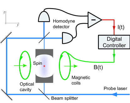
Figure 1: Schematic of an experiment for continuous quantum measurement and control. The spin interacts with an optical mode, which is measured continuously by homodyne detection. A magnetic field is used for feedback.

The model considered in this paper (Fig. 1) is prototypical for experiments in quantum optics; in fact, it is very similar to our laboratory apparatus [4]. The system consists of a cloud of atoms, collectively labeled “spin”, interacting with an optical field (along $\hat{z}$) produced by a laser. After interacting with the system the optical field is detected using a photodetector configuration known as a homodyne detector. A pair of magnetic coils (along $\hat{y}$) are used as feedback actuators.

The optical and magnetic fields are configured so they only interact, to good approximation, with the collective angular momentum degrees of freedom of all the atoms [35]. Rotational symmetry implies that observables of angular momentum must form the rotation Lie algebra $\mathfrak{so}(3)$. If we impose additionally that the total angular momentum is conserved, then it is a standard result in quantum mechanics [26] that the angular momentum observables form an irreducible representation of $\mathfrak{so}(3)$. Such a system is called a spin.

We take $\mathcal{H}$ to be the spin Hilbert space. Any finite dimension $2\leq\dim\mathcal{H}<\infty$ supports an irrep of $\mathfrak{so}(3)$; the choice of $\dim\mathcal{H}=2j+1$ depends on the number of atoms and their properties. We can choose an orthonormal basis $\{\psi_{m}\in\mathcal{H},~{}m=-j,-j+1,\ldots,j\}$ such that the observables $J_{x,y,z}$ of angular momentum around the $x,y,z$-axis are defined by

$$\begin{split}J_{x}\psi_{m}&=c_{m}\psi_{m+1}+c_{-m}\psi_{m-1}\\ J_{y}\psi_{m}&=ic_{m}\psi_{m+1}-ic_{-m}\psi_{m-1}\\ J_{z}\psi_{m}&=m\psi_{m}\end{split}$$ (37)

with $c_{m}=\tfrac{1}{2}\sqrt{(j-m)(j+m+1)}$. It is easily verified that $J_{x,y,z}$ indeed generate $\mathfrak{so}(3)$, e.g. $[J_{x},J_{y}]=iJ_{z}$.

Note that $J_{x,y,z}$ are discrete random variables; the fact that angular momentum is “quantized”, unlike in classical mechanics, is one of the remarkable predictions of quantum mechanics that give the theory its name. Another remarkable non-classical effect is that $J_{x,y,z}$ are incompatible observables.

The noise in our model and its interaction with the atoms emerges naturally from quantum electrodynamics, the quantum theory of light [36]. Physical noise is not white; however, as the correlation time of the optical noise is much shorter than the time scale of the spin dynamics, a quantum analog of the classical Wong-Zakai procedure [37, 38] can be employed to approximate the dynamics by an equation of the form (20). In fact, the term $-\tfrac{1}{2}L^{*}L$ in (20) is precisely the Wong-Zakai correction term that emerges in the white noise limit.

We now state the details of our model without further physical justification. The system is described by (20) with $L=\sqrt{M}\,J_{z}$ and $H=B(t)\,J_{y}$. Here $M>0$ is the strength of the interaction between the light and the atoms; it is regulated experimentally by the optical cavity. $B(t)$ is the applied magnetic field and serves as the control input. Finally, homodyne detection [32] provides exactly the measurement (31), where $\eta$ is determined by the efficiency of the photodetectors.

In the remainder of the paper we will study the spin system of Fig. 1. Before we devote ourselves entirely to this situation, however, we mention a couple of other common scenarios.

Often $L$ is not self-adjoint; in this case, the system can emit or absorb energy through interaction with the field. This situation occurs when the optical frequency of the cavity field is resonant with an atomic transition. In our case the frequency is chosen to be far off-resonant; this leads to self-adjoint $L$ after adiabatic elimination of the cavity dynamics (e.g. [16]). The filter dynamics in this scenario, to be described below, is known as state reduction. The sequence of approximations that is used for our particular model is described in [39].

Finally, a different detector configuration may be chosen. For example, a drastically different observation, known as photon counting, gives rise to a Poisson (jump) process. We refer to [32] for a full account of the quantum stochastic approach to observations in quantum optics.

III Geometry and dynamics of the filter

In the previous section we introduced our physical model. A detailed analysis resulted in the filtering equation (36), where $\pi_{t}(X)$ is the best estimate of the observable $X$ given the observations $Y_{s\leq t}$. We will now study this equation in detail.

Note that (36) is driven by the observation $Y_{t}$, which is a classical stochastic process. Hence (36) is entirely equivalent to a classical Itô equation. This is an important point, as it means that in the remainder of this article we only need classical stochastic calculus.

III-A The state space

We begin by investigating the state space on which the filter evolves. Clearly (36) defines the time evolution of a map $\pi_{t}$; we will show how this map can be represented efficiently.

The map $\pi_{t}$ associates to every observable $X$ on $\mathcal{H}$ a classical stochastic process which represents the expectation of $X$ conditioned on the observations up to time $t$. It is easily verified that $\pi_{t}$ is linear, identity-preserving, and maps positive observables to positive numbers: in fact, it acts exactly like the expectation of $X$ with respect to some finite-dimensional state on $\mathcal{H}$. We will denote this state by $\rho_{t}$, the conditional density at time $t$, where by definition $\pi_{t}(X)={\rm Tr}[\rho_{t}X]$.

It is straightforward to find an expression for $\rho_{t}$. We get

$$d\rho_{t}=\mathcal{L}^{*}\rho_{t}\,dt+\sqrt{\eta}(L\rho_{t}+\rho_{t}L^{*}-{\rm Tr}[\rho_{t}(L+L^{*})]\rho_{t})\,dW_{t}$$ (38)

with the innovations $dW_{t}=dY_{t}-\sqrt{\eta}{\rm Tr}[\rho_{t}(L+L^{*})]\,dt$ and the adjoint generator $\mathcal{L}^{*}\rho=-i[H,\rho]+L\rho L^{*}-\tfrac{1}{2}(L^{*}L\rho+\rho L^{*}L)$. In physics this equation is also known as a quantum trajectory equation or stochastic master equation.

Let $\dim\mathcal{H}=n$; as $n$ is finite, we can represent linear operators on $\mathcal{H}$ by complex matrices. Thus (38) is an ordinary, finite-dimensional Itô equation. We saw in section II-A that $\rho_{t}$ is a density matrix, i.e. it belongs to the space

$$\mathcal{P}=\{\rho\in\mathbb{C}^{n\times n}:\rho=\rho^{*},~{}{\rm Tr}\rho=1,~{}\rho\geq 0\}.$$ (39)

By construction $\mathcal{P}$ is an invariant set of (38), and forms the natural state space of the filter.

III-B Geometry of $\mathcal{P}$

The geometry of $\mathcal{P}$ is rather complicated [40]. To make the space more manageable we will reparametrize $\mathcal{P}$ so it can be expressed as a semialgebraic set.

Let us choose the matrix elements $\rho_{ij}$ of $\rho$ as follows. For $i>j$ set $\rho_{ij}=\lambda_{ij}+i\mu_{ij}$ with $\lambda_{ij},\mu_{ij}\in\mathbb{R}$. For $i<j$ set $\rho_{ij}=\rho_{ji}^{*}$. Finally, choose an integer $k$ between $1$ and $n$. For $i\neq k$ set $\rho_{ii}=\nu_{i}$, $\nu_{i}\in\mathbb{R}$, and $\rho_{kk}=1-\sum_{i\neq k}\nu_{i}$. Collect all $n^{2}-1$ numbers $\lambda_{ij},\mu_{ij},\nu_{i}$ into a vector $\Lambda$. Then clearly the map $h:\Lambda\mapsto\rho$ is an isomorphism between $\mathbb{R}^{n^{2}-1}$ and $\{\rho\in\mathbb{C}^{n\times n}:\rho=\rho^{*},~{}{\rm Tr}\rho=1\}$.

It remains to find the subset $K\subset\mathbb{R}^{n^{2}-1}$ that corresponds to positive definite matrices. This is nontrivial, however, as it requires us to express nonnegativity of the eigenvalues of $\rho$ as constraints on $\rho_{ij}$. The problem was solved by Kimura [40] using Descartes’ sign rule and the Newton-Girard identities for symmetric polynomials; we quote the following result:

Proposition 1

Define $k_{p}(\rho)$, $p=2\ldots n$ recursively by

$$pk_{p}(\rho)=\sum_{q=1}^{p}(-1)^{q-1}\,{\rm Tr}[\rho^{q}]\,k_{p-q}(\rho)$$ (40)

with $k_{0}=k_{1}=1$. Define the semialgebraic set

$$K=\{\Lambda\in\mathbb{R}^{n^{2}-1}:k_{p}(h(\Lambda))\geq 0,~{}p=2\ldots n\}.$$ (41)

Then $h$ is an isomorphism between $K$ and $\mathcal{P}$.

Note that $2k_{2}=1-{\rm Tr}[\rho^{2}]\geq 0$ implies $\|\Lambda\|^{2}=\sum_{i}\nu_{i}^{2}+\sum_{i>j}(\lambda_{ij}^{2}+\mu_{ij}^{2})\leq{\rm Tr}[h(\Lambda)^{2}]\leq 1$. Hence $K$ is compact.

We work out explicitly the simplest case $n=2$ (spin $j=\tfrac{1}{2}$). Set $\rho_{11}=\nu$, $\rho_{22}=1-\nu$, $\rho_{21}=\lambda+i\mu=\rho_{12}^{*}$. Then

$$K_{2}=\{\Lambda=(\lambda,\mu,\nu)\in\mathbb{R}^{3}:\lambda^{2}+\mu^{2}+\nu(\nu-1)\leq 0\}.$$ (42)

This is just a solid sphere with radius $\tfrac{1}{2}$, centered at $(0,0,\tfrac{1}{2})$. The case $n=2$ is deceptively simple, however: it is the only case with a simple topology [41, 40].

We can also express (38) in terms of $\Lambda$. Specifically, we will consider the spin system $L=\sqrt{M}\,J_{z}$, $H=B(t)\,J_{y}$ in the basis $\psi_{1/2}=(1,0)$, $\psi_{-1/2}=(0,1)$ on $\mathbb{C}^{2\times 2}$. We obtain

$$\begin{split}d\lambda_{t}&=(B(t)(\nu_{t}-\tfrac{1}{2})-\tfrac{1}{2}M\lambda_{t})\,dt+\sqrt{M\eta}\,\lambda_{t}(1-2\nu_{t})\,dW_{t}\\ d\mu_{t}&=-\tfrac{1}{2}M\mu_{t}\,dt+\sqrt{M\eta}\,\mu_{t}(1-2\nu_{t})\,dW_{t}\\ d\nu_{t}&=-B(t)\lambda_{t}\,dt-2\sqrt{M\eta}\,\nu_{t}(\nu_{t}-1)\,dW_{t}.\end{split}$$ (43)

By construction, $K_{2}$ is an invariant set for this system.

III-C Convexity and pure states

Just like its classical counterpart, the set of densities $\mathcal{P}$ is convex. We have the following fundamental result:

Proposition 2

The set $\mathcal{P}$ is the convex hull of the set of pure states $\mathcal{Q}=\{vv^{*}\in\mathbb{C}^{n\times n}:v\in\mathbb{C}^{n},~{}\|v\|=1\}\subset\mathcal{P}$.

Proof:

As any $\rho\in\mathcal{P}$ is self-adjoint it can be written as $\rho=\sum_{i}\lambda_{i}v_{i}v_{i}^{*}$, where $v_{i}$ are orthonormal eigenvectors of $\rho$ and $\lambda_{i}$ are the corresponding eigenvalues. But ${\rm Tr}\rho=1,~{}\rho\geq 0$ imply that $\sum_{i}\lambda_{i}=1$ and $\lambda_{i}\in[0,1]$. Hence $\mathcal{P}\subset{\rm conv}\,\mathcal{Q}$. Conversely, it is easily verified that ${\rm conv}\,\mathcal{Q}\subset\mathcal{P}$. ∎

Pure states are the extremal elements of $\mathcal{P}$; they represent quantum states of maximal information. Note that classically extremal measures are deterministic, i.e. $\mathbb{P}[A]$ is either $0$ or $1$ for any event $A$. This is not the case for pure states $\rho=vv^{*}$, however: any event $A=ww^{*}$ with $0<\|w^{*}v\|<1$, $\|w\|=1$ will have $0<{\rm Tr}[\rho A]<1$. Thus no quantum state is deterministic, unless we restrict to a commutative algebra $\mathcal{A}$.

Intuitively one would expect that if the output $Y_{t}$ is not corrupted by independent noise, i.e. $\eta=1$, then there is no loss of information, and hence an initially pure $\rho_{0}$ would remain pure under (38). This is indeed the case. Define

$$dv_{t}=[(h_{t}L-\tfrac{1}{2}L^{*}L-\tfrac{1}{2}h_{t}^{2}-iH)\,dt+(L-h_{t})\,dW_{t}]\,v_{t}$$ (44)

where $h_{t}=\tfrac{1}{2}v_{t}^{*}(L^{*}+L)v_{t}$. Then it is easily verified that $\rho_{t}=v_{t}v_{t}^{*}$ obeys (38) with $\eta=1$. It follows that if $\eta=1$, $\mathcal{Q}$ is an invariant set of (38). In the concrete example (43) it is not difficult to verify this property directly: when $\eta=1$, the sphere $\lambda^{2}+\mu^{2}+\nu(\nu-1)=0$ is invariant under (43).

III-D Quantum state reduction

We now study the dynamics of the spin filtering equation without feedback $B(t)=0$. We follow the approach of [42].

Consider the quantity $V_{t}=\pi_{t}(J_{z}^{2})-\pi_{t}(J_{z})^{2}$. We obtain

$$\frac{d\,\mathbb{E}[V_{t}]}{dt}=-4M\eta\,\mathbb{E}[V_{t}^{2}].$$ (45)

Clearly $\mathbb{E}[V_{t}^{2}]\geq 0$, so $\mathbb{E}[V_{t}]$ decreases monotonically. But $V_{t}\geq 0$ and $\mathbb{E}[V_{t}^{2}]=0~{}{\rm iff}~{}V_{t}=0~{}{\rm a.s.}$ We conclude that

$$\lim_{t\to\infty}\mathbb{E}[V_{t}]=0$$ (46)

and hence $V_{t}\to 0~{}{\rm a.s.}$ as $t\to\infty$. But the only states $\rho\in\mathcal{P}$ with $V_{t}={\rm Tr}[J_{z}^{2}\rho]-{\rm Tr}[J_{z}\rho]^{2}=0$ are the eigenstates $\psi_{m}\psi_{m}^{*}$ of $J_{z}$. Hence in the long-time limit the conditional state collapses onto one of the eigenstates of $J_{z}$, as predicted by (5) for a “direct” measurement of $J_{z}$.

With what probability does the state collapse onto eigenstate $m$? To study this, let us calculate $\pi_{t}(\psi_{m}\psi_{m}^{*})$. We get

$$d\pi_{t}(\psi_{m}\psi_{m}^{*})=2\sqrt{M\eta}\,\pi_{t}(\psi_{m}\psi_{m}^{*})(m-\pi_{t}(J_{z}))\,dW_{t}.$$ (47)

Clearly $\pi_{t}(\psi_{m}\psi_{m}^{*})$ is a martingale, so

$$p_{m}=\mathbb{E}[\pi_{\infty}(\psi_{m}\psi_{m}^{*})]=\pi_{0}(\psi_{m}\psi_{m}^{*}).$$ (48)

We have already shown that $\rho_{\infty}$ is one of $\psi_{n}\psi_{n}^{*}$, and as the $\psi_{m}$ are orthonormal this implies that $\pi_{\infty}(\psi_{m}\psi_{m}^{*})={\rm Tr}[\rho_{\infty}\psi_{m}\psi_{m}^{*}]$ is $1$ if $n=m$ and $0$ otherwise. Thus $p_{m}$ is just the probability of collapsing onto the eigenstate $m$. But note that $\pi_{0}(\psi_{m}\psi_{m}^{*})={\rm Tr}[\rho_{0}\psi_{m}\psi_{m}^{*}]$, so (48) gives exactly the same collapse probability as the “direct” measurement (3).

We conclude that the predictions of quantum filtering theory are entirely consistent with the traditional quantum mechanics. A continuous reduction process replaces, but is asymptotically equivalent to, the instantaneous state collapse of section II-A. This phenomenon is known as quantum state reduction. We emphasize that quantum filtering is purely a statistical inference process and is obtained entirely through nondemolition measurements. Note also that state reduction occurs because $L=J_{z}$ is self-adjoint; other cases are of equal physical interest, but we will not consider them in this paper.

Physically, the filtering approach shows that realistic measurements are not instantaneous but take some finite time. The time scale of state reduction is of order $M^{-1}$, an experimentally controlled parameter. A carefully designed experiment can thus have a reduction time scale of an order attainable by modern digital electronics [43], which opens the door to both measuring and manipulating the process in real time.

IV Stabilization of spin state reduction

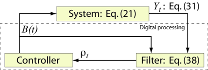
Figure 2: Schematic of the feedback control strategy. The output from the system is used to propagate the conditional state of the filter. The feedback signal is of state feedback form with respect to the conditional state.

IV-A The control problem

It is a standard idea in stochastic control that an output feedback control problem can be converted into a state feedback problem for the filter [9, 10]. This is shown schematically in Fig. 2. The filtering equations (36) or (38) are driven by $Y_{t}$; hence, at least in principle, the conditional state $\rho_{t}$ can be calculated recursively in real time by a digital processor.

The filter describes optimally our knowledge of the system; clearly the extent of our knowledge of the system state limits the precision with which it can be controlled. The best we can hope to do is to control the system to the best of our knowledge, i.e. to control the filter. The latter is a well-posed problem, despite that we cannot predict the observations $Y_{t}$, because we know the statistics of the innovations process $W_{t}$.

For such a scheme to be successful the system dynamics (21) must be known, as the optimal filter is matched to the system dynamics. Designing controllers that perform well even when the system dynamics is not known precisely is the subject of robust control theory. Also, efficient signal processing algorithms and hardware are necessary to propagate (38) in real time, which is particularly problematic when $\dim\mathcal{H}$ is large. Neither of these issues will be considered in this paper.

The state reduction dynamics discussed in the previous section immediately suggests the following control problem: we wish to find state feedback $B(t)=\Phi(\rho_{t})$ so that one of the eigenstates $\rho=\psi_{m}\psi_{m}^{*}$ is globally stabilized. The idea that a quantum measurement can be engineered to collapse deterministically onto an eigenstate of our choice is somewhat remarkable from a traditional physics perspective, but clearly the measurement scenario we have described provides us with this opportunity. For additional motivation and numerical simulations relating to this control problem, see [3].

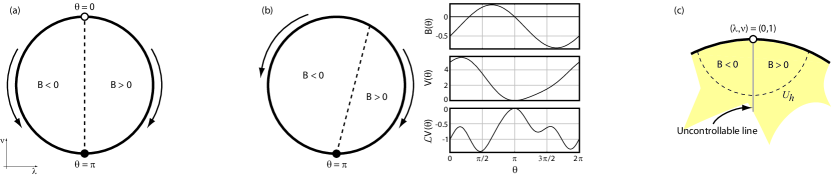
Figure 3: Cartoons of the various control schemes; the arrows denote the rotation direction of the magnetic field. (a) Almost global control on the circle: the magnetic field always rotates in the direction of least distance to $\theta=\pi$, but $\theta=0$ remains a fixed point. (b) Global control on the circle: we intentionally break the symmetry of the controller to remove the undesired fixed point. The graphs show a typical feedback law and Lyapunov design with $M=1$, $B(\theta)=\tfrac{1}{2}\sin\theta-\tfrac{1}{4}(1+\cos\theta)$, $V(\theta)=(\tfrac{5}{2}+\sin\theta)(1+\cos\theta)$. (c) A neighborhood of $(\lambda,\nu)=(0,1)$ showing why the almost global control law fails on the disc. The control vanishes on the line $\lambda=0$; hence points on this line are never repelled with unit probability, in violation of (51).

IV-B Stochastic stability

In nonlinear control theory [44] stabilization of nonlinear systems is usually performed using the powerful tools of Lyapunov stability theory. In this section we will describe the stochastic counterpart of deterministic Lyapunov theory, developed in the 1960s by Has’minskiĭ and others. We will not give proofs, for which we refer to [45, 46, 47, 48].

Let $W_{t}$ be a Wiener process on the canonical Wiener space $(\Omega,\mathcal{F},\mathbb{P})$. Consider an Itô equation on $\mathbb{R}^{n}$ of the form

$$dx_{t}=b(x_{t})\,dt+\sigma(x_{t})\,dW_{t}$$ (49)

where $b,\sigma:\mathbb{R}^{n}\to\mathbb{R}^{n}$ satisfy the usual linear growth and local Lipschitz conditions for existence and uniqueness of solutions [49]. Let $x^{*}$ be a fixed point of (49), i.e. $b(x^{*})=\sigma(x^{*})=0$.

Definition 2

The equilibrium solution $x_{t}=x^{*}$ of (49) is

1. stable in probability if

   $$\lim_{x_{0}\to x^{*}}\mathbb{P}\left[\sup_{t\geq 0}|x_{t}-x^{*}|>\epsilon\right]=0~{}~{}~{}~{}~{}~{}~{}\forall\epsilon>0,$$

2. asymptotically stable if it is stable in probability and

   $$\lim_{x_{0}\to x^{*}}\mathbb{P}\left[\lim_{t\to\infty}|x_{t}-x^{*}|=0\right]=1,$$

3. globally stable if it is stable in probability and

   $$\mathbb{P}\left[\lim_{t\to\infty}|x_{t}-x^{*}|=0\right]=1.$$

Note that 1 and 2 are local properties, whereas 3 is a global property of the system.

Recall that the infinitesimal generator of $x_{t}$ is given by

$$\mathscr{L}=\sum_{i}b^{i}(x)\frac{\partial}{\partial x^{i}}+\frac{1}{2}\sum_{ij}\sigma^{i}(x)\sigma^{j}(x)\frac{\partial^{2}}{\partial x^{i}\partial x^{j}}$$ (50)

so $d\,\mathbb{E}[f(x_{t})]/dt=\mathbb{E}[\mathscr{L}f(x_{t})]$. We can now state the stochastic equivalent of Lyapunov’s direct method [45, 46, 47].

Theorem 1

Define $U_{h}=\{x:|x-x^{*}|<h\}$. Suppose there exists some $h>0$ and a function $V:U_{h}\to\mathbb{R}_{+}$ that is continuous and twice differentiable on $U_{h}\backslash\{x^{*}\}$, such that $V(x^{*})=0$ and $V(x)>0$ otherwise, and $\mathscr{L}V(x)\leq 0$ on $U_{h}$. Then the equilibrium solution $x_{t}=x^{*}$ is stable in probability. If $\mathscr{L}V(x)<0$ on $U_{h}\backslash\{x^{*}\}$ then $x^{*}$ is asymptotically stable.

Theorem 1 is a local theorem; to prove global stability we need additional methods. When dealing with quantum filtering equations a useful global result is the following stochastic LaSalle-type theorem of Mao [48]. In the theorem we will assume that the dynamics of (49) are confined to a bounded invariant set $G$.

Theorem 2

Let $G$ be a bounded invariant set with respect to the solutions of (49) and $x_{0}\in G$. Suppose there exists a continuous, twice differentiable function $V:G\to\mathbb{R}_{+}$ such that $\mathscr{L}V(x)\leq 0$ $\forall x\in G$. Then $\lim_{t\to\infty}\mathscr{L}V(x_{t})=0~{}{\rm a.s.}$

Finally, we will find it useful to prove that a particular fixed point repels trajectories that do not originate on it. To this end we use the following theorem of Has’minskiĭ [45].

Theorem 3

Suppose there exists some $h>0$ and a function $V:U_{h}\to\mathbb{R}$ that is continuous and twice differentiable on $U_{h}\backslash\{x^{*}\}$, such that

$$\lim_{x\to x^{*}}V(x)=+\infty$$

and $\mathscr{L}V(x)<0$ on $U_{h}\backslash\{x^{*}\}$. Then the equilibrium solution $x_{t}=x^{*}$ is not stable in probability, and moreover

$$\mathbb{P}\left[\sup_{t>0}|x_{t}-x^{*}|<h\right]=0~{}~{}~{}~{}~{}~{}~{}\forall x_{0}\in U_{h}\backslash\{x^{*}\}.$$ (51)

IV-C A toy problem: the disc and the circle

We treat in detail an important toy problem: spin $j=\tfrac{1}{2}$. The low dimension and the simple topology make this problem easy to visualize. Nonetheless we will see that the stabilization problem is not easy to solve even in this simple case.

We have already obtained the filter (43) on $K_{2}$ for this case. Conveniently, the origin in $K_{2}$ is mapped to the lower eigenstate $\psi_{-1/2}\psi_{-1/2}^{*}$; we will attempt to stabilize this state.

Note that the equations for $\lambda_{t},\nu_{t}$ are decoupled from $\mu_{t}$. Moreover, the only point in $K_{2}$ with $(\lambda,\nu)=(0,0)$ has $\mu=0$. Hence we can equivalently consider the control problem

$$\begin{split}d\lambda_{t}&=(B(t)(\nu_{t}-\tfrac{1}{2})-\tfrac{1}{2}M\lambda_{t})\,dt+\sqrt{M\eta}\,\lambda_{t}(1-2\nu_{t})\,dW_{t}\\ d\nu_{t}&=-B(t)\lambda_{t}\,dt-2\sqrt{M\eta}\,\nu_{t}(\nu_{t}-1)\,dW_{t}\end{split}$$ (52)

on the disc $B^{2}=\{(\lambda,\nu)\in\mathbb{R}^{2}:\lambda^{2}+\nu(\nu-1)\leq 0\}$. Controlling (52) is entirely equivalent to controlling (43), as globally stabilizing $(\lambda,\nu)=(0,0)$ guarantees that $\mu$ is attracted to zero due to the geometry of $K_{2}$.

An even simpler toy problem is obtained as follows. Suppose $\eta=1$; we have seen that then the sphere $\lambda^{2}+\mu^{2}+\nu(\nu-1)=0$ is invariant under (43). Now suppose that additionally $\mu_{0}=0$. Then clearly the circle $S^{1}=\{(\lambda,\nu)\in\mathbb{R}^{2}:\lambda^{2}+\nu(\nu-1)=0\}$ is an invariant set. We find

$$d\theta_{t}=(B(t)-\tfrac{1}{2}M\sin\theta_{t}\cos\theta_{t})\,dt-\sqrt{M}\sin\theta_{t}\,dW_{t}$$ (53)

after a change of variables $(2\lambda_{t},2\nu_{t})=(\sin\theta_{t},1+\cos\theta_{t})$.

The system (52) could in principle be realized by performing the experiment of Fig. 1 with a single atom. The reduced system (53) is unrealistic, however: it would require perfect photodetectors and perfect preparation of the initial state. Nonetheless it is instructive to study this case, as it provides intuition which can be applied in more complicated scenarios. Note that (53) is a special case of (52) where $\eta=1$ and the dynamics is restricted to the boundary of $B^{2}$.

IV-D Almost global control on $S^{1}$

We wish to stabilize $(\lambda,\nu)=(0,0)$, which corresponds to $\theta=\pi$. Note that by (53) a positive magnetic field $B>0$ causes an increasing drift in $\theta$, i.e. a clockwise rotation on the circle. Hence a natural choice of controller is one which causes the state to rotate in the direction nearest to $\theta=\pi$ from the current position. This situation is sketched in Fig. 3a.

A drawback of any such controller is that by symmetry, the feedback must vanish not only on $\theta=\pi$ but also on $\theta=0$; hence $\theta=0$ remains a fixed point of the controlled system and the system is not globally stable. We will show, however, that under certain conditions such feedback renders the system almost globally stable, in the sense that all paths that do not start on $\theta=0$ are attracted to $\theta=\pi$ $\rm a.s.$

For simplicity we choose a controller that is linear in $(\lambda,\nu)$:

$$B(t)=2G\lambda_{t}=G\sin\theta_{t},~{}~{}~{}~{}~{}~{}~{}G>0.$$ (54)

Here $G$ is the feedback gain. The generator of (53) is then

$$\mathscr{L}=(G\sin\theta-\tfrac{1}{2}M\sin\theta\cos\theta)\frac{\partial}{\partial\theta}+\tfrac{1}{2}M\sin^{2}\theta\,\frac{\partial^{2}}{\partial\theta^{2}}.$$ (55)

As a first step we will show that the fixed point $\theta=\pi$ is asymptotically stable and that the system is always attracted to one of the fixed points (there are no limit cycles etc.) To this end, consider the Lyapunov function

$$V(\theta)=1+\cos\theta,~{}~{}~{}~{}~{}~{}~{}V(\pi)=0,~{}V(\theta\neq\pi)>0.$$ (56)

We obtain

$$\mathscr{L}V(\theta)=-G\sin^{2}\theta.$$ (57)

It follows from Theorem 1 that $\theta=\pi$ is asymptotically stable, and from Theorem 2 that $\lim_{t\to\infty}\theta_{t}\in\{0,\pi\}~{}{\rm a.s.}$

What remains to be shown is that any trajectory which does not start on $\theta=0$ ends up at $\theta=\pi~{}{\rm a.s.}$ To prove this, consider

$$\tilde{V}(\theta)=-\log(1-\cos\theta),~{}~{}~{}~{}~{}~{}~{}\lim_{\theta\to 0}\tilde{V}(\theta)=+\infty.$$ (58)

We easily find

$$\mathscr{L}\tilde{V}(\theta)=\cos^{2}(\theta/2)\,(M+M\cos\theta-2G).$$ (59)

Now note that

$$\mathscr{L}\tilde{V}(\theta)<0~{}~{}\forall\,\theta\in(-\pi,\pi)\backslash\{0\}~{}~{}~{}{\rm iff}~{}~{}~{}G\geq M.$$ (60)

Thus by Theorem 3 we have

$$\mathbb{P}\left[\sup_{t>0}|\theta_{t}|<\pi\right]=0~{}~{}~{}{\rm if}~{}~{}~{}\theta_{0}\in(-\pi,\pi)\backslash\{0\}.$$ (61)

But as $\theta\in S^{1}$ this implies $\theta_{t}\to\pi~{}{\rm a.s.}$ if $\theta_{0}\in(-\pi,\pi)\backslash\{0\}$. We conclude that the control law (54) almost globally stabilizes the system if we have sufficient gain $G\geq M$.

IV-E Global control on $S^{1}$

Any deterministic system on the circle is topologically obstructed from having a globally stabilizing controller: a continuous vector field on $S^{1}$ with a stable fixed point necessarily has an unstable fixed point as well. In the stochastic case, however, this is not the case. Though the drift and diffusion terms must each have two fixed points, we may design the system in such a way that only the stable fixed points coincide.

To apply such a trick in our system we must break the natural symmetry of the control law. This situation is shown in Fig. 3b. There is a region of the circle where the control rotates in the direction with a longer distance to $\theta=\pi$; the advantage is that $\theta=0$ is no longer a fixed point.

The linear control law that has this property has the form

$$B(t)=2G\lambda_{t}+2H\nu_{t}=G\sin\theta_{t}+H(1+\cos\theta_{t})$$ (62)

with $G>0$. We can prove global stability by applying Theorems 1 and 2 with a Lyapunov function of the form

$$V(\theta)=(\alpha+\sin\theta)(1+\cos\theta),~{}~{}~{}~{}~{}~{}~{}\alpha>1.$$ (63)

Unfortunately it is not obvious from the analytic form of $\mathscr{L}V$ how $\alpha$ must be chosen to satisfy the Lyapunov condition. It is however straightforward to plot $\mathscr{L}V$, so that in this simple case it is not difficult to search for $\alpha$ by hand.

A typical design for a particular choice of parameters is shown in Fig. 3b. The conditions of Theorems 1 and 2 are clearly satisfied, proving that the system is globally stable. Note that when the symmetry is broken we no longer need to fight the attraction of the undesired fixed point; hence there is no lower bound on $G$. In fact, in Fig. 3b we have $G<M$.

IV-F Almost global control on $B^{2}$

Unfortunately, the simple almost global control design on $S^{1}$ does not generalize to $B^{2}$. The problem is illustrated in Fig. 3c. The controller (54) vanishes at $\theta=0$ and $\pi$, but we can prove that $\theta=0$ is repelling. On $B^{2}$, however, the control vanishes on the entire line $\lambda=0$ which becomes an invariant set of (52). But then it follows from (48) that any trajectory with $\lambda_{0}=0$, $\nu_{0}\not\in\{0,1\}$ has a nonzero probability of being attracted to either fixed point.

Consider a neighborhood $U_{h}$ of the point $(\lambda,\nu)=(0,1)$ that we wish to destabilize. For any $h>0$, however small, $U_{h}$ contains points on the line $\lambda=0$ for which $\nu<1$, and we have seen that trajectories starting at such points have a nonzero probability of being attracted to $(0,1)$. But this violates (51), so clearly we cannot prove Theorem 3 on $B^{2}$.

One could attempt to prove that all points except those with $\lambda=0$ are attracted to the origin with unit probability. The Lyapunov theory of section IV-B is not equipped to handle such a case, however, and new methods must be developed [50]. Instead, we will focus on the global control problem.

IV-G Global control on $B^{2}$ and semialgebraic geometry

Once again we consider the asymmetric control law

$$B(t)=2G\lambda_{t}+2H\nu_{t},~{}~{}~{}~{}~{}~{}~{}G>0$$ (64)

and try to show that it globally stabilizes the system. Before we can solve this problem, however, we must find a systematic method for proving global stability. Searching “by hand” for Lyapunov functions is clearly impractical in two dimensions, and is essentially impossible in higher dimensions where the state space cannot be visualized.

In fact, even if we are given a Lyapunov function $V$, testing whether $\mathscr{L}V\leq 0$ on $K$ is highly nontrivial. The problem can be reduced to the following question: is the set $\{\Lambda\in\mathbb{R}^{n^{2}-1}:\mathscr{L}V>0,~{}k_{p}(h(\Lambda))\geq 0,~{}p=2\ldots n\}$ empty? Such problems are notoriously difficult to solve and their solution is known to be NP-hard in general [51].

The following result, due to Putinar [52], suggests one way to proceed. Let $S$ be a semialgebraic set, i.e. $S=\{x\in\mathbb{R}^{m}:s_{i}(x)\geq 0,~{}i=1\ldots n\}$ with polynomial $s_{i}$. Suppose that for some $i$ the set $\{x\in\mathbb{R}^{m}:s_{i}(x)\geq 0\}$ is compact. Then any polynomial $p$ that is strictly positive on $S$ is of the form

$$p(x)=p_{0}(x)+\sum_{i=1}^{n}p_{i}(x)s_{i}(x),~{}~{}p_{k}(x)=\sum_{j}p_{kj}(x)^{2}$$ (65)

where $p_{kj}$ are polynomials; i.e., $p$ is an affine combination of the constraints $s_{i}$ and sum-of-squares polynomials $p_{k}$.

Conversely, it is easy to check that any polynomial of the form (65) is nonnegative on $S$. We may thus consider the following relaxation: instead of testing nonnegativity of a polynomial on $S$, we may test whether the polynomial can be represented in the form (65). Though it is not true that any nonnegative polynomial on $S$ can be represented in this form, Putinar’s result suggests that the relaxation is not overly restrictive. The principal advantage of this approach is that the relaxed problem can be solved in polynomial time using semidefinite programming techniques [53, 54].

The approach is easily adapted to our situation as $K$ is a semialgebraic set, and we solve the relaxed problem of testing whether $-\mathscr{L}V$ can be expressed in the form (65). In fact, the semidefinite programming approach of [53, 54] even allows us to search for polynomial $V$ such that (65) is satisfied; hence we can search numerically for a global stability proof using a computer program. Such searches are easily implemented using the Matlab toolbox SOSTOOLS [55].

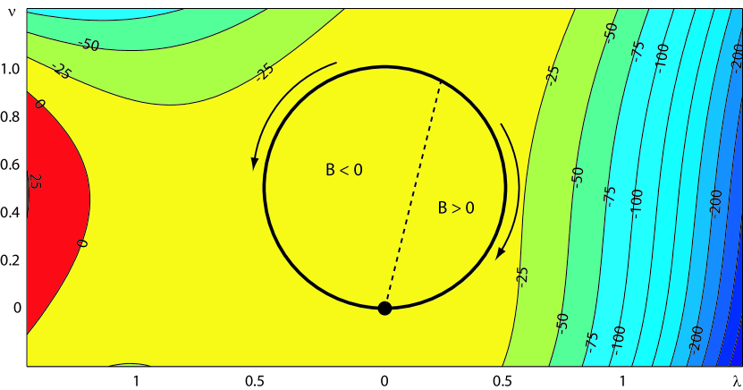
Figure 4: Contour plot of $\mathscr{L}V$ for the control law $B(t)=4\lambda_{t}-\nu_{t}$, with $M=2$ and $\eta=\tfrac{1}{2}$. The function $V$ was found by semidefinite programming.

A typical design for a particular choice of parameters is shown in Fig. 4. After fixing the parameters $M=2$, $\eta=\tfrac{1}{2}$, and the control law $B(t)=4\lambda_{t}-\nu_{t}$, an SOSTOOLS search found the Lyapunov function

$$V(\lambda,\nu)=21.8\,\nu-5.73\,\lambda^{2}+10.4\,\lambda\nu-5.63\,\nu^{2}$$ (66)

where $-\mathscr{L}V$ is of the form (65). Hence Theorems 1 and 2 are satisfied, proving that the system is globally stable.

A couple of technical points should be made at this point. Note that formally the filtering equation (38) and its parametrizations do not satisfy the linear growth condition. However, as the filter evolves on a compact invariant set $K$, we could modify the equations smoothly outside $K$ to be of linear growth without affecting the dynamics in $K$. Hence the results of section IV-B can still be used. Moreover, it is also not strictly necessary that $V$ be nonnegative, as adding a constant to $V$ does not affect $\mathscr{L}V$. Hence it is sufficient to search for polynomial $V$ using SOSTOOLS.

IV-H Global control for higher spin

The approach for proving global stability described in the previous section works for arbitrary spin $j$. To generalize our control scheme we need to convert to the parametrization of section III-B, as we did for spin $j=\tfrac{1}{2}$ in (52). We must also propose a control law that works for general spin systems.

We do not explicitly convert to the parametrized form or generate the constraints $k_{p}$, as this procedure is easily automated using Matlab’s symbolic toolbox. Note that the parameter $k$ determines which eigenstate is mapped to the origin. This is convenient for SOSTOOLS searches, as polynomials can be fixed to vanish at the origin simply by removing the constant term. We always wish to stabilize the origin in the parametrized coordinate system.

To speed up computations we can eliminate all the parameters $\mu_{ij}$ as was done in going from (43) to (52). The fact that the remaining equations are decoupled from $\mu_{ij}$ is easily seen from (38), as both $iJ_{y}$ and $J_{z}$ are real matrices. Moreover it is easily verified that, by convexity of $K$, the orthogonal projection of any $\rho\in K$ onto $\{\mathbb{R}^{n^{2}-1}:\mu_{ij}=0~{}\forall i>j\}$ lies inside $K$. Hence we only need to consider the reduced control problem with $\mu_{ij}=0$.

In [3] we numerically studied two control laws for general spin systems. The first law, $B_{1}(t)=\pi_{t}(J_{x}J_{z}+J_{z}J_{x}-2m_{d}J_{x})$ ($m_{d}$ is the eigenstate we wish to stabilize), reduces to our almost global control law when $j=\tfrac{1}{2}$. However, numerical simulations suggest that for $j>\tfrac{1}{2}$ this control law gives a finite collapse probability onto $m\neq m_{d}$. The second law, $B_{2}(t)=\pi_{t}(J_{z})-m_{d}$, reduces to $B_{2}(t)=\nu_{t}$ in the case $j=\tfrac{1}{2}$, which is not locally stable. Our experience with $j=\tfrac{1}{2}$ suggests that a control law of the form

$$B(t)=G\,\pi_{t}(J_{x}J_{z}+J_{z}J_{x}-2m_{d}J_{x})+H\,(\pi_{t}(J_{z})-m_{d})$$ (67)

should globally stabilize the eigenstate $m_{d}$ of a spin $j$ system.

We have verified global stability for a typical design with $j=1$, $M=2$, $\eta=\tfrac{1}{2}$, and $B(t)=2\,\pi_{t}(J_{x}J_{z}+J_{z}J_{x})+\pi_{t}(J_{z})$ using SOSTOOLS. A Lyapunov function was indeed found that guarantees global stability of the eigenstate $\psi_{0}\psi_{0}^{*}$.

Physically the case $j>\tfrac{1}{2}$ is much more interesting than $j=\tfrac{1}{2}$. An experiment with $j>\tfrac{1}{2}$ can be performed with multiple atoms, in which case the control produces statistical correlations between the atoms. Such correlations, known as entanglement, are important in quantum computing. The structure of the control problem is, however, essentially the same for any $j$. We refer to [3, 56] for details on entanglement generation in spin systems.

V Conclusion

In this paper we have argued that quantum mechanical systems that are subjected to measurement are naturally treated within the framework of (albeit noncommutative) stochastic filtering theory. The quantum control problem is then reduced to a classical stochastic control problem for the filter. We have demonstrated the viability of this approach by stabilizing state reduction in simple quantum spin systems using techniques of stochastic nonlinear control theory.

Unfortunately, the stabilization techniques of section IV have many drawbacks. We do not have a systematic procedure for finding control laws: we postulate linear controllers and search for corresponding Lyapunov functions. Even when the control law is known, verifying global stability is nontrivial even in the simplest case. Our numerical approach, though very successful in the examples we have shown, rapidly becomes intractable as the dimension of the Hilbert space grows. Finally, our methods do not allow us to make general statements; for example, though it seems plausible that the control law (67) is globally stabilizing for any $j,m_{d},M,\eta$, $H\neq 0$ and $G>0$, we have not yet succeeded in proving such a statement.

Nonetheless we believe that the general approach outlined in this paper provides a useful framework for the control of quantum systems. It is important in this context to develop methods for the control of classical stochastic nonlinear systems [57, 58, 59, 60], as well as methods that exploit the specific structure of quantum control problems. The design of realistic control systems will also require efficient signal processing algorithms for high-dimensional quantum filtering and methods for robust quantum control [61].

References

- [1] H. M. Wiseman and G. J. Milburn, “All-optical versus electro-optical quantum-limited feedback,” Phys. Rev. A, vol. 49, pp. 4110–4125, 1994.
- [2] M. Yanagisawa and H. Kimura, “Transfer function approach to quantum control—Part II: Control concepts and applications,” IEEE Trans. Automat. Contr., vol. 48, pp. 2121–2132, Dec. 2003.
- [3] J. K. Stockton, R. Van Handel, and H. Mabuchi, “Deterministic Dicke state preparation with continuous measurement and control,” Phys. Rev. A, vol. 70, p. 022106, 2004.
- [4] J. M. Geremia, J. K. Stockton, and H. Mabuchi, “Real-time quantum feedback control of atomic spin-squeezing,” Science, vol. 304, pp. 270–273, 2004.
- [5] E. Knill, R. Laflamme, and G. J. Milburn, “A scheme for efficient quantum computation with linear optics,” Nature, vol. 409, pp. 46–52, 2001.
- [6] H. Maassen, “Quantum probability applied to the damped harmonic oscillator,” in Quantum Probability Communications XII, S. Attal and J. M. Lindsay, Eds. World Scientific, 2003, pp. 23–58.
- [7] P. Biane, “Calcul stochastique non-commutatif,” in Lectures on Probability Theory, ser. Lecture Notes in Mathematics 1608, P. Bernard, Ed. Springer-Verlag, 1995.
- [8] P. A. Meyer, Quantum Probability for Probabilists, ser. Lecture Notes in Mathematics 1538. Springer-Verlag, 1995.
- [9] R. E. Mortensen, “Stochastic optimal control with noisy observations,” Int. J. Control, vol. 4, pp. 455–464, 1966.
- [10] K. J. Åström, “Optimal control of a Markov process with incomplete state information,” J. Math. Anal. Appl., vol. 10, pp. 174–205, 1965.
- [11] V. P. Belavkin, “Quantum stochastic calculus and quantum nonlinear filtering,” J. Multivariate Anal., vol. 42, pp. 171–201, 1992.
- [12] ——, “Quantum diffusion, measurement and filtering I,” Theory Probab. Appl., vol. 38, pp. 573–585, 1994.
- [13] ——, “Quantum continual measurements and a posteriori collapse on CCR,” Commun. Math. Phys., vol. 146, pp. 611–635, 1992.
- [14] L. Bouten, M. Guţă, and H. Maassen, “Stochastic Schrödinger equations,” J. Phys. A, vol. 37, pp. 3189–3209, 2004.
- [15] V. P. Belavkin, “Nondemolition measurements, nonlinear filtering and dynamic programming of quantum stochastic processes,” in Proceedings, Bellman Continuum, Sophia-Antipolis 1988, ser. Lecture Notes in Control and Information Sciences 121. Springer-Verlag, 1988, pp. 245–265.
- [16] A. C. Doherty and K. Jacobs, “Feedback control of quantum systems using continuous state estimation,” Phys. Rev. A, vol. 60, pp. 2700–2711, 1999.
- [17] A. C. Doherty, S. Habib, K. Jacobs, H. Mabuchi, and S. M. Tan, “Quantum feedback control and classical control theory,” Phys. Rev. A, vol. 62, p. 012105, 2000.
- [18] H. Mabuchi, J. Ye, and H. J. Kimble, “Full observation of single-atom dynamics in cavity QED,” Appl. Phys. B, vol. 68, pp. 1095–1108, 1999.
- [19] J. M. Geremia, J. K. Stockton, and H. Mabuchi. (2004) Sub-shotnoise atomic magnetometry. arXiv:quant-ph/0401107.
- [20] M. A. Armen, J. K. Au, J. K. Stockton, A. C. Doherty, and H. Mabuchi, “Adaptive homodyne measurement of optical phase,” Phys. Rev. Lett., vol. 89, p. 133602, 2002.
- [21] J. M. Geremia, J. K. Stockton, A. C. Doherty, and H. Mabuchi, “Quantum Kalman filtering and the Heisenberg limit in atomic magnetometry,” Phys. Rev. Lett., vol. 91, p. 250801, 2003.
- [22] J. K. Stockton, J. M. Geremia, A. C. Doherty, and H. Mabuchi, “Robust quantum parameter estimation: Coherent magnetometry with feedback,” Phys. Rev. A, vol. 69, p. 032109, 2004.
- [23] A. André, A. S. Sørensen, and M. D. Lukin, “Stability of atomic clocks based on entangled atoms,” Phys. Rev. Lett., vol. 92, p. 230801, 2004.
- [24] C. Ahn, A. C. Doherty, and A. J. Landahl, “Continuous quantum error correction via quantum feedback control,” Phys. Rev. A, vol. 65, p. 042301, 2002.
- [25] C. Ahn, H. M. Wiseman, and G. J. Milburn, “Quantum error correction for continuously detected errors,” Phys. Rev. A, vol. 67, p. 052310, 2003.
- [26] E. Merzbacher, Quantum Mechanics, 3rd ed. Wiley, 1998.
- [27] R. L. Hudson and K. R. Parthasarathy, “Quantum Itô’s formula and stochastic evolutions,” Commun. Math. Phys., vol. 93, pp. 301–323, 1984.
- [28] J.-M. Bismut, Mécanique Aléatoire, ser. Lecture Notes in Mathematics 866. Springer-Verlag, 1981.
- [29] L. Arnold, “The unfolding of dynamics in stochastic analysis,” Comput. Appl. Math., vol. 16, pp. 3–25, 1997.
- [30] M. H. A. Davis and S. I. Marcus, “An introduction to nonlinear filtering,” in Stochastic Systems: The Mathematics of Filtering and Identification and Applications, M. Hazewinkel and J. C. Willems, Eds. D. Reidel, 1981, pp. 53–75.
- [31] R. S. Liptser and A. N. Shiryaev, Statistics of Random Processes I: General Theory. Springer-Verlag, 2001.
- [32] A. Barchielli, “Continual measurements in quantum mechanics,” lecture notes of the Summer School on Quantum Open Systems, Institut Fourier, Grenoble, 2003.
- [33] A. S. Holevo, Probabilistic and Statistical Aspects of Quantum Theory. North-Holland, 1982.
- [34] R. Haag, Local Quantum Physics, 2nd ed. Springer-Verlag, 1996.
- [35] R. H. Dicke, “Coherence in spontaneous radiation processes,” Phys. Rev., vol. 93, pp. 99–110, 1954.
- [36] L. Mandel and E. Wolf, Optical Coherence and Quantum Optics. Cambridge University Press, 1995.
- [37] J. Gough, “Quantum flows as Markovian limit of emission, absorption and scattering interactions,” Commun. Math. Phys., 2004.
- [38] L. Accardi, A. Frigerio, and Y. G. Lu, “Weak coupling limit as a quantum functional central limit theorem,” Commun. Math. Phys., vol. 131, pp. 537–570, 1990.
- [39] L. K. Thomsen, S. Mancini, and H. M. Wiseman, “Continuous quantum nondemolition feedback and unconditional atomic spin squeezing,” J. Phys. B, vol. 35, pp. 4937–4952, 2002.
- [40] G. Kimura, “The Bloch vector for -level systems,” Phys. Lett. A, vol. 314, pp. 339–349, 2003.
- [41] K. Życzkowski and W. Słomczyński, “The Monge metric on the sphere and geometry of quantum states,” J. Phys. A, vol. 34, pp. 6689–6722, 2001.
- [42] S. L. Adler, D. C. Brody, T. A. Brun, and L. P. Hughston, “Martingale models for quantum state reduction,” J. Phys. A, vol. 34, pp. 8795–8820, 2001.
- [43] J. K. Stockton, M. A. Armen, and H. Mabuchi, “Programmable logic devices in experimental quantum optics,” J. Opt. Soc. Am. B, vol. 19, pp. 3019–3027, 2002.
- [44] H. Nijmeijer and A. Van Der Schaft, Nonlinear Dynamical Control Systems. Springer-Verlag, 1990.
- [45] R. Z. Has’minskiĭ, Stochastic Stability of Differential Equations. Sijthoff & Noordhoff, 1980.
- [46] H. J. Kushner, Stochastic Stability and Control. Academic Press, 1967.
- [47] L. Arnold, Stochastic Differential Equations: Theory and Applications. John Wiley & Sons, 1974.
- [48] X. Mao, “Stochastic versions of the LaSalle theorem,” J. Diff. Eq., vol. 153, pp. 175–195, 1999.
- [49] L. C. G. Rogers and D. Williams, Diffusions, Markov Processes and Martingales, Volume 2: Itô calculus, 2nd ed. Cambridge University Press, 2000.
- [50] R. Van Handel. (2004) Almost global stochastic stability. arXiv:math/0411311.
- [51] P. A. Parrilo, “Semidefinite programming relaxations for semialgebraic problems,” Math. Prog. B, vol. 96, pp. 293–320, 2003.
- [52] M. Putinar, “Positive polynomials on compact semi-algebraic sets,” Indiana Univ. Math. J., vol. 42, pp. 969–984, 1993.
- [53] P. A. Parrilo, “Structured semidefinite programs and semialgebraic geometry methods in robustness and optimization,” 2000, Ph.D. thesis, Calif. Inst. Technol., Pasadena, CA.
- [54] A. Papachristodoulou and S. Prajna, “On the construction of Lyapunov functions using the sum of squares decomposition,” Proc. 41st IEEE CDC, vol. 3, pp. 3482–3487, 2002.
- [55] S. Prajna, A. Papachristodoulou, P. Seiler, and P. A. Parrilo, “SOSTOOLS: Sum of squares optimization toolbox for Matlab,” Available from http://www.cds.caltech.edu/sostools.
- [56] J. K. Stockton, J. M. Geremia, A. C. Doherty, and H. Mabuchi, “Characterizing the entanglement of symmetric multi-particle spin-1/2 systems,” Phys. Rev. A, vol. 67, p. 022112, 2003.
- [57] P. Florchinger, “A universal formula for the stabilization of control stochastic differential equations,” Stoch. Anal. Appl., vol. 11, pp. 155–162, 1993.
- [58] ——, “Lyapunov-like techniques for stochastic stability,” SIAM J. Control Optim., vol. 33, pp. 1151–1169, 1995.
- [59] ——, “Feedback stabilization of affine in the control stochastic differential systems by the control Lyapunov function method,” SIAM J. Control Optim., vol. 35, pp. 500–511, 1997.
- [60] ——, “A stochastic Jurdjevic-Quinn theorem,” SIAM J. Control Optim., vol. 41, pp. 83–88, 2002.
- [61] M. R. James, “Risk-sensitive optimal control of quantum systems,” Phys. Rev. A, vol. 69, p. 032108, 2004.