Quantum Entanglement in Time

Abstract

The temporal Bell inequalities are derived from the assumptions of realism and locality in time. It is shown that quantum mechanics violates these inequalities and thus is in conflict with the two assumptions. This can be used for performing certain tasks that are not possible classically. Our results open up a possibility for introducing the notion of entanglement in time in quantum physics.

Conceptually, as well as mathematically, space and time are differently described in quantum mechanics. While time enters as an external parameter in the dynamical evolution of a system, spatial coordinates are regarded as quantum-mechanical observables. Moreover, spatially separated quantum systems are associated with the tensor product structure of the Hilbert state-space of the composite system. This allows a composite quantum system to be in a state that is not separable regardless of the spatial separation of its components. We speak about entanglement in space. On the other hand, time in quantum mechanics is normally regarded as lacking such a structure.

Entanglement in space displays one of the most interesting features of quantum mechanics, often called quantum nonlocality. Locality in space and realism impose constraints - Bell’s inequalities bell - on certain combinations of correlations for measurements of spatially separated systems, which are violated by quantum mechanics. Furthermore, entanglement in space is considered as a resource that allows powerful new communication and computational tasks that are not possible classically nielsen .

Because of different roles time and space play in quantum theory one could be tempted to assume that the notion of “entanglement in time” cannot be introduced in quantum physics. In this letter we will investigate this question and we will find that this is not the case.

We will explicitly derive temporal Bell’s inequalities (the notion of temporal Bell’s inequalities was first introduced by Leggett and Garg leggett in a different context; see discussion below) in analogy to the spatial ones. They are constraints on certain combinations of temporal correlations for measurements of a single quantum system, which are performed at different times. We explicitly show that quantum mechanics violates these inequalities. While mathematically two-fold correlations in space and in time are equivalent, the general spatial and temporal $m$-fold correlations can have completely different features. On one hand, every $m$-fold temporal correlation is decomposable into two-fold correlations, so that no Bell’s inequalities that detect genuine $m$-fold $(m\!>\!2)$ nonseparability svetlichny can be violated. On the other hand, and in apparent contradiction with this, the temporal correlations may be stronger than the spatial ones in a certain sense. Finally, we show that entanglement in time can save on the size of classical memory required in certain computational problems beyond the classical limits.

The temporal Bell’s inequalities are derived from the following two assumptions freewill : (a) Realism: The measurement results are determined by ”hidden” properties the particles carry prior to and independent of observation, and (b) Locality in time: The results of measurement performed at time $t_{2}$ are independent of any measurement performed at some earlier or later time $t_{1}$. It should be noted that in contrast to spatial correlations, where the special theory of relativity can be invoked to ensure locality in space, no such principle exists to ensure locality in time for temporal correlations. Nevertheless, it is meaningful to ask whether or not the quantum-mechanical predictions are compatible with the assumptions (a) and (b). Ultimately we expect to learn more about the relation between the structure of space and time and the abstract formalism of quantum theory.

We comment on important related works leggett ; paz . While there temporal Bell’s inequalities are for histories, our inequalities are for predetermined measurement values. Also, there the observer measures a single observable having a choice between different times $t_{i}$ of measurement (the times $t_{i}$ play the role of measurement settings), whereas in our case at any given time $t_{i}$ the observer has a choice between different measurement settings. We will see that the possibility of the observer to choose between different observables is decisive for our new computational task that is not possible classically.

We shall now derive the temporal analog of the Clauser-Horne-Shimony-Holt (CHSH) inequality chsh from the assumptions (a) and (b). Consider an observer and allow her to choose at time $t_{i}$ to measure between two dichotomic observables, determined by some parameters $\vec{n}^{1}_{i}$ and $\vec{n}^{2}_{i}$. The assumptions (a) and (b) imply existence of numbers $A_{t_{i}}(\vec{n}^{1}_{i})$ and $A_{t_{i}}(\vec{n}^{2}_{i})$ each taking values either +1 or -1, which describe the predetermined result of the measurement performed at time $t_{i}$ of the observable defined by $\vec{n}^{1}_{i}$ and $\vec{n}^{2}_{i}$, respectively.

In a specific sequence of $m$ measurements performed at the set of times $t_{1},...,t_{m}$, the correlations between $m$ observations are given by the product $\prod_{j=1}^{m}A_{t_{j}}(\vec{n}^{k_{j}}_{j})$, with $k_{j}\!=\!1,2$. The temporal correlation function is then the average over many runs of the sequence of measurements, as given by $E(\vec{n}^{k_{1}}_{1},...,\vec{n}^{k_{m}}_{m})\!=\!\langle\prod_{j=1}^{m}A_{t_{j}}(\vec{n}^{k_{j}}_{i})\rangle_{avg}$.

In what follows we will consider only correlations for measurements performed at two different times $t_{1}$ and $t_{2}$. To avoid too many indices we introduce a new notation for predetermined values: $A^{1}_{t_{1}}$ and $A^{2}_{t_{1}}$ stand for the measurement results at time $t_{1}$ for the observables $\vec{a}_{1}$ and $\vec{a}_{2}$, and $B^{1}_{t_{2}}$ and $B^{2}_{t_{2}}$ are the results at time $t_{2}$ for $\vec{b}_{1}$ and $\vec{b}_{2}$, respectively. The following algebraic identity holds for the predetermined values: $A^{1}_{t_{1}}(B^{1}_{t_{2}}+B^{2}_{t_{2}})+A^{2}_{t_{1}}(B^{1}_{t_{2}}-B^{2}_{t_{2}})=\pm 2.$ After averaging this expression over many runs of the sequence of measurements, one obtains the temporal CHSH inequality

$$B\equiv|E(\vec{a}_{1},\vec{b}_{1})+E(\vec{a}_{1},\vec{b}_{2})+E(\vec{a}_{2},\vec{b}_{1})-E(\vec{a}_{2},\vec{b}_{2})|\leq 2$$ (1)

in analogy to the spatial one. We call expression $B$ on the left-hand side of ineq. (1) the Bell expression. Note that probability distribution in phase space in classical mechanics satisfy this inequality.

We will now calculate the temporal correlation function for consecutive measurements of a single qubit. An arbitrary mixed state of a qubit can be written as $\rho=\frac{1}{2}(\mathbb{I}+\vec{r}\cdot\vec{\sigma})$, where $\mathbb{I}$ is the identity operator, $\vec{\sigma}\equiv(\sigma_{x},\sigma_{y},\sigma_{z})$ are the Pauli operators for three orthogonal directions $x$, $y$ and $z$, and $\vec{r}\equiv(r_{x},r_{y},r_{z})$ is the Bloch vector with the components $r_{i}\!=\!\mbox{Tr}(\rho\sigma_{i})$. Here ”$\cdot$” denotes the ordinary scalar product in a three-dimensional Euclidian space.

Suppose that the measurement of the observable $\vec{\sigma}\cdot\vec{a}$ is performed at time $t_{1}$, followed by the measurement of $\vec{\sigma}\cdot\vec{b}$ at $t_{2}$, where $\vec{a}$ and $\vec{b}$ are directions at which spin is measured. The quantum correlation function is given by $E_{QM}(\vec{a},\vec{b})=\sum_{k,l=\pm 1}k\cdot l\cdot\mbox{Tr}(\rho P^{k}_{\vec{a}})\cdot\mbox{Tr}(P^{k}_{\vec{a}}P^{l}_{\vec{b}}),$ where, e.g., $P^{k}_{\vec{a}}$ is the projector onto the subspace corresponding to the eigenvalue $k\!=\!\pm 1$ of the spin along $\vec{a}$. Here we use the fact that after the first measurement the state is projected on the new state $P^{k}_{\vec{a}}$. Therefore, the probability to obtain the result $k$ in the first measurement and $l$ in the second one is given by $\mbox{Tr}(\rho P^{k}_{\vec{a}})\cdot\mbox{Tr}(P^{k}_{\vec{a}}P^{l}_{\vec{b}})$. Using $P^{k}_{\vec{a}}=\frac{1}{2}(\mathbb{I}+k\vec{\sigma}\cdot\vec{a})$ and $\frac{1}{2}\mbox{Tr}[(\vec{\sigma}\cdot\vec{a})(\vec{\sigma}\cdot\vec{b})]=\vec{a}\cdot\vec{b}$ one can easily show that the quantum correlation function can simply be written as

$$E_{QM}(\vec{a},\vec{b})=\vec{a}\cdot\vec{b}.$$ (2)

It is remarkable that in contrast to the spatial correlation function the temporal one (2) does not dependent of the initial state $\rho$. We note that our derivation of Eq. (2), if one adopts Heisenbergs picture, also includes the cases where the system evolves under arbitrary unitary transformation between the two measurements.

We shall now show that quantum mechanics violates the temporal CHSH inequality and is thus in conflict with the assumptions (a) and (b). We compute the quantum value $B_{QM}$ for the Bell expression where the observer can choose between observables $(\vec{\sigma}\cdot\vec{a}_{1})$ and $(\vec{\sigma}\cdot\vec{a}_{2})$ at time $t_{1}$ and between $(\vec{\sigma}\cdot\vec{b}_{1})$ and $(\vec{\sigma}\cdot\vec{b}_{2})$ at $t_{2}$. We obtain

$$B_{QM}=|\vec{a}_{1}\cdot(\vec{b}_{1}+\vec{b}_{2})+\vec{a}_{2}\cdot(\vec{b}_{1}-\vec{b}_{2})|.$$ (3)

The maximal violation of the temporal CHSH inequality is achieved for the choice of the measurement settings: $\vec{a}_{1}\!=\!\frac{1}{\sqrt{2}}(\vec{b}_{1}+\vec{b}_{2})$ and $\vec{a}_{1}\!=\!\frac{1}{\sqrt{2}}(\vec{b}_{1}-\vec{b}_{2})$ and is equal to $2\sqrt{2}$. This can be called the temporal Cirel’son bound cirelson .

We now consider the situation of three consecutive observations. We are still interested in two-fold correlations for two measurements performed, say, at times $t_{1}$ and $t_{3}$, but where an additional measurement is performed at time $t_{2}$ lying between $t_{1}$ and $t_{3}$ ($t_{1}\!<\!t_{2}\!<\!t_{3}$). Suppose that the three measurements are: $(\vec{\sigma}\cdot\vec{a})$ at time $t_{1}$, $(\vec{\sigma}\cdot\vec{b})$ at $t_{2}$ and $(\vec{\sigma}\cdot\vec{c})$ at $t_{3}$. Applying the similar method as used for computing Eq. (2) one obtains:

$$E_{QM}(\vec{a},\vec{c}) = \sum_{k,l,s=\pm 1}k\cdot s\cdot\mbox{Tr}(\rho P^{k}_{\vec{a}})\cdot\mbox{Tr}(P^{k}_{\vec{a}}P^{l}_{\vec{b}})\cdot\mbox{Tr}(P^{l}_{\vec{b}}P^{s}_{\vec{c}})$$ (4)

$$= (\vec{a}\cdot\vec{b})(\vec{b}\cdot\vec{c})$$

for the correlation for measurements performed at times $t_{1}$ and $t_{3}$. One can convince oneself that the correlation function (4) for a given measurement performed at $t_{2}$ cannot violate the temporal CHSH inequality for measurements at $t_{1}$ and $t_{3}$. Therefore, any measurement performed at time $t_{2}$ “disentangles” events at times $t_{1}$ and $t_{3}$ if $t_{1}\!<\!t_{2}\!<\!t_{3}$.

It should be noted that the temporal correlation as given by Eq. (2) (with a minus sign in front) can also be obtained for results of the consecutive measurements of two qubits that are in the maximally entangled state (singlet). We will see, however, that the equivalence between spatial and temporal correlations is not a general feature, but rather a peculiarity of the two-fold correlations. In fact, the quantum correlation $E_{QM}(\vec{n}_{1},...,\vec{n}_{m})$ for measurements performed at $m$ instances of time $t_{1},...,t_{m}$ is decomposable into a product of two-fold temporal correlations of the type (2). One obtains

$$E_{QM}(\vec{n}_{1},...,\vec{n}_{m})=$$

$$\sum_{s_{1},...,s_{m}=\pm 1}s_{1}...s_{m}\mbox{Tr}(\rho P^{s_{1}}_{\vec{n}_{1}})\mbox{Tr}(P^{s_{1}}_{\vec{n}_{1}}P^{s_{2}}_{\vec{n}_{2}})...\mbox{Tr}(P^{s_{m-1}}_{\vec{n}_{m-1}}P^{s_{m}}_{\vec{n}_{m}})$$

$$= E_{QM}(\vec{n}_{1},\vec{n}_{2})\cdot E_{QM}(\vec{n}_{3},\vec{n}_{4})\cdot...\cdot E_{QM}(\vec{n}_{m-1},\vec{n}_{m}),$$

where we assume that $m$ is even for simplicity. This implies that, in contrast to general spatial correlation, correlation in time is partially separable, i.e. any $m$ events in time are composed of sets of pairs of events which may be correlated in any way (e.g. entangled) within the pair but which are uncorrelated with respect to the events from other pairs. Consequently, the Bell-type inequalities that detect genuine $m$-fold nonseparability svetlichny are satisfied by the temporal correlations for all $m\!>\!2$.

One can understand this in the following way. With the only exception being when the system is in an eigenstate of the measured observable, the set of future probabilistic predictions specified by the new projected state is indifferent to the knowledge collected from the previous measurements in the whole history of the system. One has only correlations between the state preparation, which also can be considered as a measurement of the system at time $t_{i}$, and the measurement performed at the next time $t_{i+1}$. A related view was held by Pauli pauli who wrote (see translation for translation): “Bei Ubestimmheit einer Eigenschaft eines Systems bei einer bestimmten Anordnung (bei einem bestimmten Zustand des Systems) vernichtet jeder Versuch, die betreffende Eigenschaft zu messen, (mindestend teilweise) den Einfluß der früheren Kenntnisse von System auf die (eventuell statistischen) Aussagen über spätere mögliche Messungsergebnisse.”

Although in contrast to correlations in space there are no genuine multi-mode correlations in time, we will see that temporal correlations can be stronger than spatial ones in a certain sense. We denote by $\max{[B^{space}_{QM}(i,j)]}$ the maximal value of the Bell expression for qubits $i$ and $j$. Scarani and Gisin scarani found an interesting bound that holds for arbitrary state of three qubits:

$$\max{[B^{space}_{QM}(1,2)]}+\max{[B^{space}_{QM}(2,3)]}\leq 4.$$ (6)

Physically, this means that no two pairs of qubits of a three-qubit system can violate the CHSH inequalities simultaneously. This is because if two systems are highly entangled, they cannot be entangled highly to another systems. Let us denote by $\max{[B^{time}_{QM}(1,2)]}$ the maximal value of the Bell expression for two consecutive observations of a single qubit at times $i$ and $j$. Since temporal two-fold correlations (2) do not depend on the initial state one can simply combine them to obtain

$$\max{[B^{time}_{QM}(1,2)]}+\max{[B^{time}_{QM}(2,3)]}\leq 4\sqrt{2}.$$ (7)

Thus, although there are no genuine 3-fold temporal correlations, a specific combination of two-fold correlations can have values that are not achievable with correlations in space for any 3-qubit system. In fact, one would need two pairs of maximally entangled two-qubit states (two e-bits) to achieve the bound in (7). Also note that the local realistic bound is 4, which is equal to the bound in (6) but lower than the one in (7). Similar conclusion can be obtained for the sum of $m$ Bell’s expressions.

We now show that entanglement in time can be used to perform certain tasks that are not possible classically. With “classically” we mean here compatible with the assumptions (a) and (b). Our tasks are temporal analogue of communication complexity problems yao ; buhrman ; brukner ; brassard with space and time interchanging roles. Consider a party who receives a set of input data $z_{1},...,z_{m}$ at different times $t_{1},...,t_{m}$, respectively. The goal for her is to determine the value of a certain function $f(z_{1},...,z_{m})$ that depends on all data. During the protocol she is allowed to use random strings that are classically correlated in time, which might improve the success of the protocol. Obviously, if the party has enough memory to store all $m$ inputs, she can compute the function with certainty after receiving all inputs. We will consider the problem: What is the highest possible probability for the party to arrive at the correct value of the function if only a restricted amount of the (classical) memory is available? We will show that there are functions $f$ for which the party can increase the success rate, if she uses entanglement in time rather than random strings correlated classically in time.

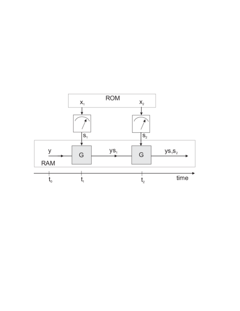
Figure 1: Quantum protocol for computing the function given in Eq. (8). The size of the RAM is restricted to 1 bit. A party receives input bits $y,x_{1},x_{2}$ at times $t_{0},t_{1},t_{2}$, respectively (e.g. from the computer ROM). She has a qubit system and a suitable device for measuring two-valued observables. The input $y$ is feed into RAM. Depending on the specific value $x_{i}$, $i=1,2$ of her input, the party chooses to measure between two different observables. Applying the gate $G$ the result $s_{i}$ of the measurement is multiplied by the previous bit value of the RAM. The final output is $y\cdot s_{1}\cdot s_{2}$.

We will consider a function introduced previously in the framework of communication complexity buhrman ; brukner . Imagine that the party receives bit input $y\!\in\!(-1,1)$ at time $t_{0}$, $x_{1}\!\in\!(0,1)$ at $t_{1}$, and finally $x_{2}\!\in\!(0,1)$ at $t_{2}$. One can imagine that she has an access to her ROM (read-only memory - computer memory whose contents can be only be read out) where the inputs are stored only at times $t_{i}$, $i=0,1,2$. Her goal is to compute the function

$$f(y,x_{1},x_{2})=y\cdot(-1)^{x_{1}x_{2}}$$ (8)

with as high probability as possible, while having only amount of 1 bit of memory (RAM) available. In other words, the size of her RAM (random-access memory - computer memory which can be used to perform necessary tasks) is restricted to 1 bit.

We will first present a quantum protocol and then show that it is more efficient than any classical one. The party receives the input $y$ at time $t_{0}$ and feeds it into her RAM as shown in Fig. 1. If at time $t_{1}$ she receives $x_{1}\!=\!0$, she will measure an observable $(\vec{\sigma}\cdot\vec{a}_{1})$ on her qubit. For $x_{1}\!=\!1$, she will measure $(\vec{\sigma}\cdot\vec{a}_{2})$. The actual value $\pm 1$ obtained in the measurement is denoted by $s_{1}$. The party uses a multiplication gate $G$ to multiply the value $y$ of the bit in the RAM with the measurement result $s_{1}$. She obtains $y\!\cdot\!s_{1}$ as the new value in her RAM. The same strategy is repeated also at time $t_{2}$ with the measurement of observable $(\vec{\sigma}\cdot\vec{b}_{1})$ or $(\vec{\sigma}\cdot\vec{b}_{2})$ and the actual result denoted by $s_{2}$. As the final output the party obtains $y\cdot s_{1}\cdot s_{2}$.

The probability of the success of the quantum protocol is equal to the probability $P$ for the product $s_{1}\cdot s_{2}$ to be equal to $(-1)^{x_{1}x_{2}}$. This probability can be written as

$$P = \frac{1}{4}[P_{\vec{a}_{1},\vec{b}_{1}}(s_{1}s_{2}\!=\!1)+P_{\vec{a}_{1},\vec{b}_{2}}(s_{1}s_{2}\!=\!1)$$ (9)

$$+ P_{\vec{a}_{2}\vec{b}_{1}}(s_{1}s_{2}\!=\!1)+P_{\vec{a}_{2},\vec{b}_{2}}(s_{1}s_{2}\!=\!-1)],$$

where, e.g., $P_{\vec{a}_{1},\vec{b}_{2}}(s_{1}s_{2}\!=\!1)$ is the probability that $s_{1}s_{2}\!=\!1$ if the party receives input value $x_{1}\!=\!0$ at $t_{1}$ and $x_{2}\!=\!1$ at $t_{2}$. All four possible input combinations occur with the same probability $1/4$.

It is important to see that the probability of success can be expressed as $P\!=\!\frac{1}{4}B$, where $B$ is the Bell expression given in (1). On the other hand, a classical protocol, that is any protocol that is compatible with the assumptions (a) and (b), can be understood as exploiting a realistic and local-in-time model of the quantum protocol. This implies that the probability of the success in any classical protocol comment is bounded, i.e. $P_{C}\leq 3/4\!=\!75\%$. The quantum protocol will have higher success if and only if the choice of the pair of measurements at time $t_{1}$ and $t_{2}$ violates the temporal CHSH inequality. With the optimal choice of the measurements the probability of success is $P_{Q}\!=\!85\%$. Note that to achieve this success rate classically one has to use at least the size of two bits of the memory (RAM).

We note that one can also construct tasks whose quantum solutions would exploit violation of the classical bound for the expression (7). Not only that those tasks would not be possible classically but they also could not be efficiently performed with spatial entanglement without additional resources (e-bits). Finally, we note that quantum communication complexity protocols that are not based on entanglement but on exchange of qubits yao ; brassard can also be reformulated within the framework of our tasks. Note, however, that here we are interested in exchanging classical bits rather than qubits. This exploits entanglement in time as a resource for increasing capacities of classical computational devices.

One related issue we have not explored in this paper is that of mathematically describing time by associating a tensor product structure to a sequence of time instances. This seems to be necessitated by our notion of entanglement in time. Finkelstein was first to consider something similar when he introduced quantised instances of time called chronons finkelstein . More recently, Isham, within the framework of consistent histories, explored the same possibility isham . It is clear from our work, however, that it is very difficult to extend the tensor product structure beyond the two neighbouring instances in time without altering the basic principles of quantum mechanics. In fact, one of the features of entanglement in time is exactly a consequence of this difficulty: two maximally entangled events can still be maximally entangled to two other events in time (a principle we may call “polygamy” of entanglement in time). This is in contrast to the spatial entanglement which can only be “monogamous” bennett . The difference between the spatial and temporal structure may ultimately be fundamental, or it may be an indication that we need a deeper theory in which the two need to be treated on a more equal footing (quantum field theory does not suffice in this sense). Either way, it appears that the next step should lie in exploring the consequences of combining entanglement in space and time in order to study how they relate to each other.

- (1)
- (2) J.S. Bell, Physics (Long Island City, N.Y.) 1, 195 (1964).
- (3) M.A. Nielsen and I.L. Chuang, Quantum Computation and Quantum Information (Cambridge University, 2000).
- (4) A.J. Leggett and A. Garg, Phys. Rev. Lett. 54, 857 (1985).
- (5) M. Seevinck and G. Svetlichny, Phys. Rev. Lett. 89, 060401 (2002). D. Collins, N. Gisin, S. Popescu, D. Roberts and V. Scarani, Phys. Rev. Lett. 88, 170405 (2002).
- (6) The assumption of “free-will” - the freedom of the observer to choose the measurement setting - is implicitely assumed.
- (7) J.P. Paz and G. Mahler, Phys. Rev. Lett. 71, 3235 (1993).
- (8) J. Clauser , M. Horne, A. Shimony, and R. Holt, Phys. Rev. Lett. 23, 880 (1969).
- (9) W. Pauli, in Handbuch der Physik, edited by S. Flügge (Springer-Verlag, Berlin, 1958), Band Vol. 1, p. 7.
- (10) B.S. Cirel’son, Lett. Math. Phys. 4, 93 (1980).
- (11) “In the case of undefiniteness of a property of a system for a certain arrangement (with certain state of the system) any attempt to measure that specific property destroys (at least partially) the influence of earlier knowledge of the system on (possibly statistical) statements about later possible measurement results.”
- (12) V. Scarani and N. Gisin, Phys. Rev. Lett. 87, 117901 (2001).
- (13) A. C.-C. Yao, in Proc. of the 11th Annual ACM Symposium on Theory of Computing, 209 (1979). A. C.-C. Yao, in Proc. of the 34th Annual IEEE Symposium in Foundations of Computer Science, 1993, 352.
- (14) H. Buhrman, R. Cleve and W. van Dam, e-print quant-ph/9705033.
- (15) Č. Brukner, M. Żukowski, J.-W. Pan and A. Zeilinger, in print in Phys. Rev. Lett., e-print quant-ph/0210114.
- (16) One can show that even if one considers the most general classical protocols cannot exceed 75%. The proof is along the similar lines as the one in Ref. brukner .
- (17) See G. Brassard, e-print quant-ph/0101005 for a survey and references therein. See also E. F. Galvao, Phys. Rev. A65, 012318 (2002).
- (18) D. Finkelstein, Phys. Rev. 184, 1261 (1969).
- (19) C. J. Isham, J. Math. Phys. 35, 2157 (1994).
- (20) As far as we are aware Bennett was the first to introduce the notion of “monogamy” of entanglement.