Extremal entanglement and mixedness in continuous variable systems

Abstract

We investigate the relationship between mixedness and entanglement for Gaussian states of continuous variable systems. We introduce generalized entropies based on Schatten $p$-norms to quantify the mixedness of a state, and derive their explicit expressions in terms of symplectic spectra. We compare the hierarchies of mixedness provided by such measures with the one provided by the purity (defined as ${\rm tr}\,\varrho^{2}$ for the state $\varrho$) for generic $n$-mode states. We then review the analysis proving the existence of both maximally and minimally entangled states at given global and marginal purities, with the entanglement quantified by the logarithmic negativity. Based on these results, we extend such an analysis to generalized entropies, introducing and fully characterizing maximally and minimally entangled states for given global and local generalized entropies. We compare the different roles played by the purity and by the generalized $p$-entropies in quantifying the entanglement and the mixedness of continuous variable systems. We introduce the concept of average logarithmic negativity, showing that it allows a reliable quantitative estimate of continuous variable entanglement by direct measurements of global and marginal generalized $p$-entropies.

I Introduction

The degree of entanglement (i.e. the contents in quantum correlations) as well as the degree of mixedness (i.e.  “the amount” by which a state fails to be pure) are among the crucial features of quantum states from the point of view of quantum information theory. Indeed, the search for proper analytical ways to quantify such features for general (mixed) quantum states cannot be yet considered accomplished. In view of such considerations, it is clear that the full understanding of the relationships between the quantum correlations contained in a bipartite state and the global and local (i.e. referring to the reduced states of the two subsystems) degrees of mixedness of the state, would be desirable. In particular, it would be a relevant step towards the clarification of the nature of quantum correlations and, possibly, of the distinction between quantum and classical correlations of mixed states, which remains an open issue henvedral01 . A simple question one can raise in such a context is the investigation of the properties of extremally entangled states for a given degree of mixedness.

Let us mention that, as for two–qubit systems, the notion of maximally entangled states at fixed mixedness (MEMS) was originally introduced by Ishizaka and Hiroshima hishizaka00 . The discovery of such states spurred several theoretical works vers01 , aimed at exploring the relations between different measures of entanglement and mixedness wei03 (strictly related to the question of the ordering of these different measures order ). Moreover, maximally entangled states for given local (or “marginal”) mixednesses have been recently introduced and analyzed in detail in the context of qubit systems adesso03 . On the experimental side, much attention has been devoted to exploring the two-qubit Hilbert space in optical settings white02 , while the experimental realization of MEMS has been recently demonstrated demartonzo03 .

Because of the great current interest in continuous variable (CV) quantum information pati03 ; crypto ; tele ; dense , the extension of such analyses to infinite dimensional systems is higly desirable. In the present work, we introduce and study in detail extremally entangled mixed Gaussian states of infinite dimensional Hilbert spaces for fixed global and marginal generalized entropies, significantly generalizing the results derived earlier in Ref. adeser04 , where the existence of maximally and minimally entangled mixed Gaussian states at given global and marginal purities was first discovered. In the present paper we will make use of a hierarchy of generalized entropies, based on the Schatten $p$-norms, to quantify mixedness and characterize extremal entanglement in continuous varibale (CV) systems and investigate several related subjects, like the ordering of such different entropic measures and the relations between EPR (Einstein-Podolsky-Rosen) correlations and symplectic spectra. The crucial starting point of our analysis is the observation that the existence of infinitely entangled states jens02 ; keylwer prevents maximally entangled Gaussian states from being defined as states with maximal, finite, logarithmic negativity, even at fixed global mixedness foot1 . However, we will show that fixing the global and the local mixednesses allows to define unambiguously both maximally and minimally entangled mixed Gaussian states. This relevant and somehow surprising result – there is no analog of Gaussian minimally entangled states in finite dimensional systems – turns out to have an experimental interest as well adeser04 ; fiurcerf03 .

The paper is structured as follows. In Sec. II we briefly review the basic notation and the general properties of Gaussian states. In Sec. III we introduce the hierarchy of generalized Schatten $p$-norms and entropies, and we extensively discuss the problem of the ordering of different entropic measures for states with an arbitrary number of modes. In Sec. IV we review the state of the art on the existing, computable measures of entanglement for two–mode Gaussian states, while in Sec. V we present a heuristic argument relating EPR correlations to symplectic spectra. In Sec. VI we introduce a parametrization of two–mode Gaussian states in terms of symplectic invariants endowed with a direct physical interpretation. Exploiting these results, in Sec. VII we define maximally and minimally entangled states for given global and marginal purities and present some experimental situations in which these states occur. In Sec. VIII we generalize the concept of extremal entanglement in CV systems by introducing maximally and minimally entangled states for given global and local generalized entropies of arbitrary order, and we present an extensive study of their properties. We find out, somehow surprisingly, that maximally and minimally entangled states can interchange their roles for certain ranges of values of the global and marginal $p$-entropies; moreover, we observe that with increasing $p$ the generalized entropies, while carrying in general less information on a quantum state, provide a more accurate quantification of its entanglement. In Sec. IX we introduce and study the concept of “average logarithmic negativity”, showing that this quantity provides an excellent quantitative estimate of CV entanglement based only on the knowledge of global and local entropies. Finally, in Sec. X we summarize our results and discuss future perspectives.

II Gaussian states: general overview

Let us consider a CV system, described by an Hilbert space ${\cal H}=\bigotimes_{i=1}^{n}{\cal H}_{i}$ resulting from the tensor product of the infinite dimensional Fock spaces ${\cal H}_{i}$’s. Let $a_{i}$ be the annihilation operator acting on ${\cal H}_{i}$, and $\hat{x}_{i}=(a_{i}+a^{{\dagger}}_{i})$ and $\hat{p}_{i}=(a_{i}-a^{{\dagger}}_{i})/i$ be the related quadrature phase operators. The corresponding phase space variables will be denoted by $x_{i}$ and $p_{i}$. Let us group together the operators $\hat{x}_{i}$ and $\hat{p}_{i}$ in a vector of operators $\hat{X}=(\hat{x}_{1},\hat{p}_{1},\ldots,\hat{x}_{n},\hat{p}_{n})$. The canonical commutation relations for the $\hat{X}_{i}$’s are encoded in the symplectic form $\boldsymbol{\Omega}$

$$[\hat{X}_{i},\hat{X}_{j}]=2i\Omega_{ij}\;,$$

$${\rm with}\quad\boldsymbol{\Omega}\equiv\bigoplus_{i=1}^{n}\boldsymbol{\omega}\;,\quad\boldsymbol{\omega}\equiv\left(\begin{array}[]{cc}0&1\\ -1&0\end{array}\right)\;.$$

The set of Gaussian states is, by definition, the set of states with Gaussian characteristic functions and quasi–probability distributions. Therefore a Gaussian state $\varrho$ is completely characterized by its first and second statistical moments, which form, respectively, the vector of first moments $\bar{X}\equiv\left(\langle\hat{X}_{1}\rangle,\langle\hat{X}_{1}\rangle,\ldots,\langle\hat{X}_{n}\rangle,\langle\hat{X}_{n}\rangle\right)$ and the covariance matrix of elements $\boldsymbol{\sigma}$

$$\sigma_{ij}\equiv\frac{1}{2}\langle\hat{X}_{i}\hat{X}_{j}+\hat{X}_{j}\hat{X}_{i}\rangle-\langle\hat{X}_{i}\rangle\langle\hat{X}_{j}\rangle\,,$$ (1)

where, for any observable $\hat{o}$, the expectation value $\langle\hat{o}\rangle\equiv\,{\rm Tr}(\varrho\hat{o})$. First statistical moments can be arbitrarily adjusted by local unitary operations, which cannot affect any property related to entanglement or mixedness. Therefore they will be unimportant to our aims and we will set them to $0$ in the following, without any loss of generality. Throughout the paper, $\boldsymbol{\sigma}$ will stand for the covariance matrix of the Gaussian state $\varrho$.

Let us now consider the hermitian operator $\hat{y}=Y\hat{X}^{T}$, where $Y\in\mathbb{R}^{2n}$ is an arbitrary real $2n$-dimensional row vector. Positivity of $\varrho$ imposes ${\rm Tr}(\varrho\hat{y}^{2})\geq 0$, which can be simply recast in terms of second moments as $Y\boldsymbol{\tau}Y^{T}\geq 0$, with $\tau_{ij}=\langle\hat{X}_{i}\hat{X}_{j}\rangle$. From this relation, exploiting the canonical commutation relations and recalling definition (1) and the arbitrarity of $Y$, the Heisenberg uncertainty principle can be recast in the form

$$\boldsymbol{\sigma}+i\boldsymbol{\Omega}\geq 0\;,$$ (2)

Inequality (2) is the necessary and sufficient constraint $\boldsymbol{\sigma}$ has to fulfill to be a bona fide covariance matrix simon87 ; simon94 . We mention that such a constraint implies $\boldsymbol{\sigma}\geq 0$.

In the following, we will make use of the Wigner quasi–probability representation $W(x_{i},p_{i})$ defined, for any density matrix, as the Fourier transform of the symmetrically ordered characteristic function barnett . In Wigner phase space picture, the tensor product ${\cal H}=\bigotimes{\cal H}_{i}$ of the Hilbert spaces ${\cal H}_{i}$’s of the $n$ modes results in the direct sum $\Gamma=\bigoplus\Gamma_{i}$ of the phase spaces $\Gamma_{i}$’s. In general, as a consequence of the Stone-von Neumann theorem, any symplectic transformation acting on the phase space $\Gamma$ corresponds to a unitary operator acting on the Hilbert space $\cal H$, through the so called metaplectic representation. Such a unitary operator is generated by terms of the second order in the field operators simon94 . In what follows we will refer to a transformation $S_{l}=\bigoplus S_{i}$, with each $S_{i}\in Sp_{(2,\mathbb{R})}$ acting on $\Gamma_{i}$, as to a “local symplectic operation”. The corresponding unitary transformation is the “local unitary transformation” $U_{l}=\bigotimes U_{i}$, with each $U_{i}$ acting on ${\cal H}_{i}$.

The Wigner function of a Gaussian state can be written as follows in terms of phase space quadrature variables

$$W(X)=\frac{\,{\rm e}^{-\frac{1}{2}X\boldsymbol{\sigma}^{-1}X^{T}}}{\pi\sqrt{{\rm Det}\,\boldsymbol{\sigma}}}{\>,}$$ (3)

where $X$ stands for the vector $(x_{1},p_{1},\ldots,x_{n},p_{n})\in\Gamma$.

Finally let us recall that, due to Williamson theorem williamson36 , the covariance matrix of a $n$–mode Gaussian state can always be written as simon87

$$\boldsymbol{\sigma}=S^{T}\boldsymbol{\nu}S\;,$$ (4)

where $S\in Sp_{(2n,\mathbb{R})}$ and $\boldsymbol{\nu}$ is the covariance matrix

$$\boldsymbol{\nu}=\,{\rm diag}({\nu}_{1},{\nu}_{1},\ldots,{\nu}_{n},{\nu}_{n})\,,$$ (5)

corresponding to a tensor product of thermal states with diagonal density matrix $\varrho^{{}_{\otimes}}$ given by

$$\varrho^{{}_{\otimes}}=\bigotimes_{i}\frac{2}{\nu_{i}+1}\sum_{k=0}^{\infty}\left(\frac{\nu_{i}-1}{\nu_{i}+1}\right)|k\rangle_{i}{}_{i}\langle k|\;,$$ (6)

$|k\rangle_{i}$ being the $k$-th number state of the Fock space ${\cal H}_{i}$. The dual (Hilbert space) formulation of Eq. (4) then reads: $\varrho=U^{{\dagger}}\,\varrho^{{}_{\otimes}}\,U$, for some unitary $U$.
The quantities $\nu_{i}$’s form the symplectic spectrum of the covariance matrix $\boldsymbol{\sigma}$ and can be computed as the eigenvalues of the matrix $|i\boldsymbol{\Omega}\boldsymbol{\sigma}|$. Such eigenvalues are in fact invariant under the action of symplectic transformations on the matrix $\boldsymbol{\sigma}$.
The symplectic eigenvalues $\nu_{i}$ encode essential informations on the Gaussian state $\boldsymbol{\sigma}$ and provide powerful, simple ways to express its fundamental properties. For instance, let us consider the Heisenberg uncertainty relation (2). Since $S$ is symplectic, one has $S^{-1T}\boldsymbol{\Omega}S^{-1}=\boldsymbol{\Omega}$, so that inequality (2) is equivalent to $\boldsymbol{\nu}+i\boldsymbol{\Omega}\geq 0$. In terms of the symplectic eigenvalues $\nu_{i}$ the uncertainty relation then simply reads

$${\nu}_{i}\geq 1\;.$$ (7)

We can, without loss of generality, rearrange the modes of a $n$-mode state such that the corresponding symplectic eigenvalues are sorted in ascending order

$$\nu_{1}\leq\nu_{2}\leq\ldots\leq\nu_{n-1}\leq\nu_{n}\,.$$

With this notation, the uncertainty relation reduces to $\nu_{1}\geq 1$. We remark that the full saturation of Heisenberg uncertainty principle can only be achieved by pure $n$-mode Gaussian states, for which $\nu_{i}=1\,\,\forall i=1,\ldots,n$. Instead, mixed states such that $\nu_{i\leq k}=1$ and $\nu_{i>k}>1$, with $1\leq k\leq n$, only partially saturate the uncertainty principle, with partial saturation becoming weaker with decreasing $k$. Such states are minimum uncertainty mixed Gaussian states in the sense that the phase quadrature operators of the first $k$ modes satisfy the Heisenberg minimal uncertainty, while for the remaining $n-k$ modes the state indeed contains some additional thermal and/or Schrödinger–like correlations which are responsible for the global mixedness of the state.

II.1 Two–mode states

In the present work we will mainly deal with two–mode Gaussian states. Here, we will thus briefly review their relevant properties and specify some further notations.

The expression of the two–mode covariance matrix $\boldsymbol{\sigma}$ in terms of the three $2\times 2$ matrices $\boldsymbol{\alpha}$, $\boldsymbol{\beta}$, $\boldsymbol{\gamma}$ will be useful

$$\boldsymbol{\sigma}\equiv\left(\begin{array}[]{cc}\boldsymbol{\alpha}&\boldsymbol{\gamma}\\ \boldsymbol{\gamma}^{T}&\boldsymbol{\beta}\end{array}\right)\,.$$ (8)

It is well known that for any two–mode covariance matrix $\boldsymbol{\sigma}$ there exists a local symplectic operation $S_{l}=S_{1}\oplus S_{2}$ which takes $\boldsymbol{\sigma}$ to the so called standard form $\boldsymbol{\sigma}_{sf}$ simon00 ; duan00

$$S_{l}^{T}\boldsymbol{\sigma}S_{l}=\boldsymbol{\sigma}_{sf}\equiv\left(\begin{array}[]{cccc}a&0&c_{+}&0\\ 0&a&0&c_{-}\\ c_{+}&0&b&0\\ 0&c_{-}&0&b\end{array}\right)\;.$$ (9)

States whose standard form fulfills $a=b$ are said to be symmetric. Let us recall that any pure state is symmetric and fulfills $c_{+}=-c_{-}=\sqrt{a^{2}-1}$. The correlations $a$, $b$, $c_{+}$, and $c_{-}$ are determined by the four local symplectic invariants ${\rm Det}\boldsymbol{\sigma}=(ab-c_{+}^{2})(ab-c_{-}^{2})$, ${\rm Det}\boldsymbol{\alpha}=a^{2}$, ${\rm Det}\boldsymbol{\beta}=b^{2}$, ${\rm Det}\boldsymbol{\gamma}=c_{+}c_{-}$. Therefore, the standard form corresponding to any covariance matrix is unique.

The uncertainty principle Ineq. (2) can be recast as a constraint on the $Sp_{(4,{\mathbb{R}})}$ invariants ${\rm Det}\boldsymbol{\sigma}$ and $\Delta(\boldsymbol{\sigma})={\rm Det}\boldsymbol{\alpha}+\,{\rm Det}\boldsymbol{\beta}+2\,{\rm Det}\boldsymbol{\gamma}$:

$$\Delta(\boldsymbol{\sigma})\leq 1+\,{\rm Det}\boldsymbol{\sigma}\;.$$ (10)

Let us mention that, as it is evident from Eq. (9), the condition $\boldsymbol{\sigma}\geq 0$ implies

$$ab-c_{\mp}^{2}\geq 0\;.$$ (11)

The symplectic eigenvalues of a two–mode Gaussian state will be named $\nu_{-}$ and $\nu_{+}$, with $\nu_{-}\leq\nu_{+}$ in general. With such an ordering, the Heisenberg uncertainty relation Eq. (7) becomes

$$\nu_{\mp}\geq 1\;.$$ (12)

Full saturation $\nu_{-}=\nu_{+}=1$ yields the standard pure Gaussian states of Heisenberg minimum uncertainty; partial saturation $\nu_{-}=1$, $\nu_{+}>1$ defines the minimum-uncertainty mixed Gaussian states. A simple expression for the $\nu_{\mp}$ can be found in terms of the two $Sp_{(4,\mathbb{R})}$ invariants vidwer ; serafozzi

$$2{\nu}_{\mp}^{2}=\Delta(\boldsymbol{\sigma})\mp\sqrt{\Delta(\boldsymbol{\sigma})^{2}-4\,{\rm Det}\,\boldsymbol{\sigma}}\,.$$ (13)

In turn, Eq. (13) yields immediately

$$\Delta(\boldsymbol{\sigma})\,=\,{\nu}_{-}^{2}\,+\,{\nu}_{+}^{2}\;.$$ (14)

A subclass of Gaussian states that will play a relevant role in the following is constituted by the nonsymmetric two–mode squeezed thermal states. Let $S_{r}=\exp(\frac{1}{2}ra_{1}a_{2}-\frac{1}{2}ra_{1}^{{\dagger}}a_{2}^{{\dagger}})$ be the two mode squeezing operator with real squeezing parameter $r$, and let $\varrho^{{}_{\otimes}}_{\nu_{i}}$ be a tensor product of thermal states with covariance matrix ${\boldsymbol{\nu}}_{\nu_{\mp}}={\mathbbm{1}}_{2}\nu_{-}\oplus{\mathbbm{1}}_{2}\nu_{+}$, where $\nu_{\mp}$ is, as usual, the symplectic spectrum of the state. Then, a nonsymmetric two-mode squeezed thermal state $\xi_{\nu_{i},r}$ is defined as ${\xi}_{\nu_{i},r}=S_{r}\varrho^{{}_{\otimes}}_{\nu_{i}}S_{r}^{{\dagger}}$, corresponding to a standard form with

$$a = {\nu_{-}}\cosh^{2}r+{\nu_{+}}\sinh^{2}r\;,$$

$$b = {\nu_{-}}\sinh^{2}r+{\nu_{+}}\cosh^{2}r\;,$$ (15)

$$c_{\pm} = \pm\frac{\nu_{-}+\nu_{+}}{2}\sinh 2r\;.$$

We mention that the peculiar entanglement properties of squeezed nonsymmetric thermal states have been recently analyzed jiang03 . In the symmetric instance (with $\nu_{-}=\nu_{+}=\nu$) these states reduce to two–mode squeezed thermal states. The covariance matrices of these states are symmetric standard forms with

$$a=\nu\,{\cosh 2r}\;,\quad c_{\pm}=\pm\nu\,{\sinh 2r}\,.$$ (16)

In the pure case, for which $\nu=1$, one recovers the two–mode squeezed vacua. Notice that such states encompass all the standard forms associated to pure states: any two–mode Gaussian state can reduced to a squeezed vacuum by means of unitary local operations.
Two–mode squeezed states (both thermal and pure) are endowed with remarkable properties related to entanglement 2max ; giedke03 ; rigesc03 . Even the ideal, perfectly correlated original EPR state epr35 can be seen indeed as a two–mode squeezed vacuum in the limit of infinite squeezing parameter $r$. The dynamical properties of the entanglement and the characterization of the decoherence of such states have been addressed in detail in several works dumodi . We will also show, as a byproduct of the present work, the peculiar role they play as maximally entangled Gaussian states.

III Measures of mixedness, degree of coherence, and entropic measures

The degree of mixedness of a quantum state $\varrho$ can be characterized completely by the knowledge of all the associated Schatten $p$–norms bathia

$$\|\varrho\|_{p}\equiv(\,{\rm Tr}\,|\varrho|^{p})^{\frac{1}{p}}=(\,{\rm Tr}\,\varrho^{p})^{\frac{1}{p}}\,,\quad\,{\rm with}\>p\geq 1.$$ (17)

In particular, the case $p=2$ is directly related to the purity $\mu=\,{\rm Tr}\,\varrho^{2}=(\|\varrho\|_{2})^{2}$ paris . The $p$-norms are multiplicative on tensor product states and thus determine a family of “generalized entropies” $S_{p}$ bastiaans ; tsallis , defined as

$$S_{p}=\frac{1-\,{\rm Tr}\,\varrho^{p}}{p-1}\;,\quad p>1.$$ (18)

These quantities have been introduced independently by M. J. Bastiaans in the context of quantum optics bastiaans , and by C. Tsallis in the context of statistical mechanics tsallis . In the quantum arena, they can be interpreted both as quantifiers of the degree of mixedness of a state $\varrho$ by the amount of information it lacks, and as measures of the overall degree of coherence of the state (the latter meaning was elucidated by Bastiaans in his analysis of the properties of partially coherent light). The quantity $S_{2}=1-\mu\equiv S_{L}$, conjugate to the purity $\mu$, is usually referred to as the linear entropy: it is a particularly important measure of mixedness, essentially because of the simplicity of its analytical expressions, which will become soon manifest. Finally, another important class of entropic measures includes the Rényi entropies renyi

$$S_{p}^{R}=\frac{\ln\,{\rm Tr}\,\varrho^{p}}{1-p}\;,\quad p>1.$$ (19)

It can be easily shown that

$$\lim_{p\rightarrow 1+}S_{p}=\lim_{p\rightarrow 1+}S_{p}^{R}=-\,{\rm Tr}\,(\varrho\ln\varrho)\equiv S_{V}\,,$$ (20)

so that also the Shannon-von Neumann entropy $S_{V}$ can be defined in terms of $p$-norms. The quantity $S_{V}$ is additive on tensor product states and provides a further convenient measure of mixedness of the quantum state $\varrho$.

It is easily seen that the generalized entropies $S_{p}$’s range from $0$ for pure states to $1/(p-1)$ for completely mixed states with fully degenerate eigenspectra. Notice that $S_{V}$ is infinite on infinitely mixed states, while $S_{L}$ is normalized to $1$. We also mention that, in the asymptotic limit of arbitrary large $p$, the function $\,{\rm Tr}\,\varrho^{p}$ becomes a function only of the largest eigenvalue of $\varrho$: more and more information about the state is discarded in such an estimate for the degree of purity; considering $S_{p}$ in the limit $p\rightarrow\infty$ yields a trivial constant null function, with no information at all about the state under exam. We also note that, for any given quantum state, $S_{p}$ is a monotonically decreasing function of $p$.

Because of their unitarily invariant nature, the generalized purities ${\rm Tr}\,\varrho^{p}$ of generic $n$–mode Gaussian states can be simply computed in terms of the symplectic eigenvalues $\nu_{i}$ of $\boldsymbol{\sigma}$. In fact, a symplectic transformation acting on $\boldsymbol{\sigma}$ is embodied by a unitary (trace preserving) operator acting on $\varrho$, so that ${\rm Tr}\,\varrho^{p}$ can be easily computed on the diagonal state $\nu$. One obtains

$${\rm Tr}\,\varrho^{p}=\prod_{i=1}^{n}g_{p}(\nu_{i})\;,$$ (21)

where

$$g_{p}(x)=\frac{2^{p}}{(x+1)^{p}-(x-1)^{p}}\,.$$

A first consequence of Eq. (21) is that

$$\mu(\varrho)=\frac{1}{\prod\nu_{i}}=\frac{1}{\sqrt{{\rm Det}\,\boldsymbol{\sigma}}}\,.$$ (22)

Regardless of the number of modes, the purity of a Gaussian state is fully determined by the symplectic invariant ${\rm Det}\,\boldsymbol{\sigma}$ alone. A second consequence of Eq. (21) is that, together with Eqs. (18) and (20), it allows for the computation of the von Neumann entropy $S_{V}$ of a Gaussian state $\varrho$, yielding

$$S_{V}(\varrho)=\sum_{i=1}^{n}f(\nu_{i})\;,$$ (23)

where

$$f(x)\equiv\frac{x+1}{2}\ln\left(\frac{x+1}{2}\right)-\frac{x-1}{2}\ln\left(\frac{x-1}{2}\right)\,.$$

Such an expression for the von Neumann entropy of a Gaussian state was first explicitly given in Ref. holevo99 . Let us remark that, clearly, the symplectic spectrum of single mode Gaussian states, which consists of only one eigenvalue $\nu_{1}$, is fully determined by the invariant ${\rm Det}\,\boldsymbol{\sigma}=\nu_{1}^{2}$ Therefore, all the entropies $S_{p}$’s (and $S_{V}$ as well) are just increasing functions of ${\rm Det}\,\boldsymbol{\sigma}$ (i.e. of $S_{L}$) and induce the same hierarchy of mixedness on the set of one–mode Gaussian states. This is no longer true for multi–mode states, even for the relevant, simple instance of two–mode states.

Here we aim to find extremal values of $S_{p}$ (for $p\neq 2$) for fixed $S_{L}$ in the general $n$–mode Gaussian instance, in order to quantitatively compare the characterization of mixedness given by the different entropic measures. For simplicity, in calculations we will replace $S_{L}$ with $\mu$. In view of Eqs. (21) and (22), the possible values taken by $S_{p}$ for a given $\mu$ are determined by

$$(p-1)S_{p}=1-\left(\prod_{i=1}^{n-1}g_{p}(s_{i})\right)g_{p}\left(\frac{1}{\mu\prod_{i=1}^{n-1}s_{i}}\right)\,,$$ (24)

$${\rm with}\quad 1\leq s_{i}\leq\frac{1}{\mu\prod_{i\neq j}s_{j}}\,.$$ (25)

The last constraint on the $n-1$ real auxiliary parameters $s_{i}$ is a consequence of the uncertainty relation (7). We first focus on the instance $p<2$, in which the function $S_{p}$ is concave with respect to any $s_{i}$, for any value of the $s_{i}$’s. Therefore its minimum with respect to, say, $s_{n-1}$ occurs at the boundaries of the domain, for $s_{n-1}$ saturating inequality (25). Since $S_{p}$ takes the same value at the two extrema and exploiting $g_{p}(1)=1$, one has

$$(p-1)\min_{s_{n-1}}S_{p}=1-\left(\prod_{i=1}^{n-2}g_{p}(s_{i})\right)g_{p}\left(\frac{1}{\mu\prod_{i=1}^{n-2}s_{i}}\right)\>.$$ (26)

Iterating this procedure for all the $s_{i}$’s leads eventually to the minimum value $S_{p\,min}(\mu)$ of $S_{p}$ at given purity $\mu$, which simply reads

$$S_{p\,min}(\mu)=\frac{1-g_{p}\left(\frac{1}{\mu}\right)}{p-1}\,,\quad p<2\,.$$ (27)

For $p<2$, the mixedness of the states with minimal generalized entropies at given purity is therefore concentrated in one quadrature: the symplectic spectrum of such states is partially degenerate, with $\nu_{1}=\ldots=\nu_{n-1}=1$ and $\nu_{n}=1/\mu$.

The maximum value $S_{p\,max}(\mu)$ is achieved by states satisfying the coupled trascendental equations

$$g_{p}\left(\frac{1}{\mu\prod s_{i}}\right)g^{\prime}_{p}(s_{j})=\frac{1}{\mu s_{j}\prod s_{i}}\,g_{p}(s_{j})g^{\prime}_{p}\left(\frac{1}{\mu\prod s_{i}}\right)\,,$$ (28)

where all the products $\prod$ run over the index $i$ from $1$ to $n-1$, and

$$g^{\prime}_{p}(x)=\frac{-p\,2^{p}\left[(x+1)^{p-1}-(x-1)^{p-1}\right]}{\left[(x+1)^{p}-(x-1)^{p}\right]^{2}}\,.$$ (29)

It is promptly verified that the above two conditions are fulfilled by states with a completely degenerate symplectic spectrum: $\nu_{1}=\ldots=\nu_{n}={\mu}^{-1/n}$, yielding

$$S_{p\,max}(\mu)=\frac{1-g_{p}\left(\mu^{-\frac{1}{n}}\right)^{n}}{p-1}\,,\quad p<2\,.$$ (30)

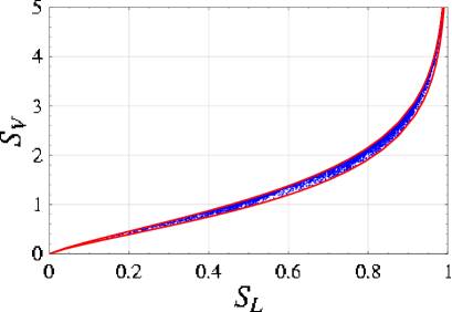
The analysis that we carried out for $p<2$ can be straightforwardly extended to the limit $p\rightarrow 1$, yielding the extremal values of the von Neumann entropy for given purity $\mu$ of $n$–mode Gaussian states. Also in this case the states with maximal $S_{V}$ are those with a completely degenerate symplectic spectrum, while the states with minimal $S_{V}$ are those with all the mixedness concentrated in one quadrature. The extremal values $S_{Vmin}(\mu)$ and $S_{Vmax}(\mu)$ read

$$S_{Vmin}(\mu) = f\left(\frac{1}{\mu}\right)\;,$$ (31)

$$S_{Vmax}(\mu) = nf\left(\mu^{-\frac{1}{n}}\right)\;.$$ (32)

The behaviors of the von Neumann and of the linear entropies for two–mode states are compared in Fig. 1.

Figure 1: Plot of the curves (solid lines) of maximal and minimal von Neumann entropy at given linear entropy for two–mode Gaussian states. The density of states in the plane of entropies is represented as well, by plotting the distribution of 20000 randomly generated states (dots).

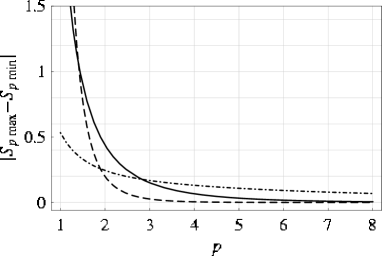
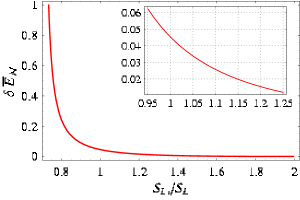
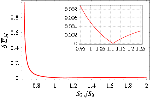
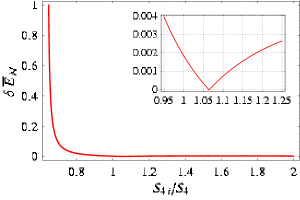
The instance $p>2$ can be treated in the same way, with the major difference that the function $S_{p}$ of Eq. (24) is convex with respect to any $s_{i}$ for any value of the $s_{i}$’s. As a consequence we have an inversion of the previous expressions: for $p>2$, the states with minimal $S_{p\,min}(\mu)$ at given purity $\mu$ are those with a fully distributed symplectic spectrum, with

$$S_{p\,min}(\mu)=\frac{1-g_{p}\left(\mu^{-\frac{1}{n}}\right)^{n}}{p-1}\,,\quad p>2\,.$$ (33)

On the other hand, the states with maximal $S_{p\,max}$ at given purity $\mu$ are those with a spectrum of the kind $\nu_{1}=\ldots=\nu_{n-1}=1$ and $\nu_{n}=1/\mu$. Therefore

$$S_{p\,max}(\mu)=\frac{1-g_{p}\left(\frac{1}{\mu}\right)}{p-1}\,,\quad p>2\,.$$ (34)

As shown in Fig. 2, the distance $|S_{p\,max}-S_{p\,min}|$ decreases with increasing $p$. This is due to the fact that the quantity $S_{p}$ carries less information with increasing $p$, and the knowledge of $\mu$ provides a more precise bound on the value of $S_{p}$.

Figure 2: Plot of the absolute difference between the maximal and the minimal values of the generalized entropies $S_{p}$ at fixed linear entropy $S_{L}$ for two–mode Gaussian states, as a function of $p$. Different curves correspond to different values of the linear entropy: $S_{L}=0.8$ (dashed line), $S_{L}=0.5$ (continuous line), and $S_{L}=0.1$ (dash-dotted line).

IV Measures of Entanglement

We now review the main aspects of entanglement for CV systems and discuss some of the possible quantifications of quantum correlations for Gaussian states.

The necessary and sufficient separability criterion for a two–mode Gaussian state $\varrho$ has been shown to be positivity of the partially transposed state $\tilde{\varrho}$ (PPT criterion) simon00 . In general, the partial transposition $\tilde{\varrho}$ of a bipartite quantum state $\varrho$ is defined as the result of the transposition performed on only one of the two subsystems in some given basis. Even though the resulting $\tilde{\varrho}$ does depend on the choice of the transposed subsystem and on the transposition basis, the statement $\tilde{\varrho}\geq 0$ is geometric, and is invariant under such choices perhor . It can be easily seen from the definition of $W(X)$ that the action of partial transposition amounts, in phase space, to a mirror reflection of one of the four canonical variables. In terms of $Sp_{(2,\mathbb{R})}\oplus Sp_{(2,\mathbb{R})}$ invariants, this reduces to a sign flip in ${\rm Det}\,\boldsymbol{\gamma}$

$${\rm Det}\,\boldsymbol{\gamma}\;\;\xrightarrow{\,\,\varrho\rightarrow\tilde{\varrho}\,\,}\;\;-{\rm Det}\,\boldsymbol{\gamma}\;.$$

Therefore the invariant $\Delta(\boldsymbol{\sigma})$ is changed into $\tilde{\Delta}({\boldsymbol{\sigma}})=\Delta(\tilde{\boldsymbol{\sigma}})=\,{\rm Det}\,\boldsymbol{\alpha}+\,{\rm Det}\,\boldsymbol{\beta}-2\,{\rm Det}\,\boldsymbol{\gamma}$. Now, the symplectic eigenvalues $\tilde{\nu}_{\mp}$ of $\tilde{\boldsymbol{\sigma}}$ read

$$\tilde{\nu}_{\mp}=\sqrt{\frac{\tilde{\Delta}(\boldsymbol{\sigma})\mp\sqrt{\tilde{\Delta}(\boldsymbol{\sigma})^{2}-4\,{\rm Det}\,\boldsymbol{\sigma}}}{2}}\,.$$ (35)

The PPT criterion thus reduces to a simple inequality that must be satisfied by the smallest symplectic eigenvalue $\tilde{\nu}_{-}$ of the partially transposed state

$$\tilde{\nu}_{-}\geq 1\>,$$ (36)

which is equivalent to

$$\tilde{\Delta}(\boldsymbol{\sigma})\leq\,{\rm Det}\,\boldsymbol{\sigma}+1\;.$$ (37)

The above inequalities imply ${\rm Det}\,\boldsymbol{\gamma}=c_{+}c_{-}<0$ as a necessary condition for a two–mode Gaussian state to be entangled. The quantity $\tilde{\nu}_{-}$ encodes all the qualitative characterization of the entanglement for arbitrary (pure or mixed) two–modes Gaussian states. Note that $\tilde{\nu}_{-}$ takes a particularly simple form for entangled symmetric states, whose standard form has $a=b$

$$\tilde{\nu}_{-}=\sqrt{(a-|c_{+}|)(a-|c_{-}|)}\;.$$ (38)

Inserting Eqs. (15) into Eq. (37) yields the following condition for a two-mode squeezed thermal state $\xi_{\nu_{i},r}$ to be entangled

$$\sinh^{2}(2r)>\frac{(\nu_{+}^{2}-1)(\nu_{-}^{2}-1)}{(\nu_{-}+\nu_{+})^{2}}\;.$$ (39)

As for the quantification of entanglement, no fully satisfactory measure is known at present for arbitrary mixed bipartite Gaussian states. However, a quantification of entanglement which can be computed for general Gaussian states is provided by the negativity ${\cal N}$, first introduced in Ref. zircone , later thoroughly discussed and extended in Ref. vidwer to CV systems. The negativity of a quantum state $\varrho$ is defined as

$${\cal N}(\varrho)=\frac{\|\tilde{\varrho}\|_{1}-1}{2}\>,$$ (40)

where $\tilde{\varrho}$ is the partially transposed density matrix and $\|\hat{o}\|_{1}=\,{\rm Tr}|\hat{o}|$ stands for the Schatten $1$-norm (the so called ‘trace norm’) of the hermitian operator $\hat{o}$. The quantity ${\cal N}(\varrho)$ is equal to $|\sum_{i}\lambda_{i}|$, the modulus of the sum of the negative eigenvalues of $\tilde{\varrho}$, quantifying the extent to which $\tilde{\varrho}$ fails to be positive. Strictly related to ${\cal N}$ is the logarithmic negativity $E_{{\cal N}}$, defined as $E_{{\cal N}}\equiv\ln\|\tilde{\varrho}\|_{1}$, which constitutes an upper bound to the distillable entanglement of the quantum state $\varrho$.

The negativity has been proven to be convex and monotone under LOCC (local operations and classical communications) negnote , but fails to be continuous in trace norm on infinite dimensional Hilbert spaces. However, this problem can be circumvented by restricting to physical states with finite mean energy jens02 .

We will now show that for any two–mode Gaussian state $\varrho$ the negativity is a simple decreasing function of $\tilde{\nu}_{-}$, which is thus itself an entanglement monotone. The norm $\|\tilde{\cdot}\|_{1}$ is unitarily invariant; in particular, it is invariant under global symplectic operations in phase space. Considering the symplectic diagonalization $\boldsymbol{\tilde{\nu}}\equiv\,{\rm diag}\,(\tilde{\nu}_{-},\tilde{\nu}_{-},\tilde{\nu}_{+},\tilde{\nu}_{+})$ of $\tilde{\boldsymbol{\sigma}}$, this means that ${\cal N}(\varrho)=(\|\tilde{\nu}\|_{1}-1)/2$. Now, because of the multiplicativity of the norm $\|\cdot\|_{1}$, we have just to compute the trace of the single–mode thermal–like operator $\rho^{{}_{\otimes}}_{\tilde{\nu}_{i}}$

$$\rho^{{}_{\otimes}}_{\tilde{\nu}_{i}}=\frac{2}{\tilde{\nu}_{i}+1}\sum_{k=0}^{\infty}\left(\frac{\tilde{\nu}_{i}-1}{\tilde{\nu}_{i}+1}\right)^{k}|k\rangle\langle k|\;.$$

Such an operator is obviously normalized for $\tilde{\nu}_{i}\geq 1$, yielding $\|\rho^{{}_{\otimes}}_{\tilde{\nu}_{i}}\|_{1}=1$ (all eigenvalues are positive). Instead, if $\tilde{\nu}_{i}<1$, then $\|\rho^{{}_{\otimes}}_{\tilde{\nu}_{i}}\|_{1}=1/\tilde{\nu}_{i}$. The proof is completed by showing that the largest symplectic eigenvalue $\tilde{\nu}_{+}$ of $\tilde{\boldsymbol{\sigma}}$ fulfills $\tilde{\nu}_{+}\geq 1$. This is obviously true for separable states, therefore we can set $c_{+}c_{-}<0$. With this position, it is easy to show that

$$\tilde{\nu}_{+}>{\nu}_{-}\geq 1\;.$$

Thus, we obtain $\|\rho^{{}_{\otimes}}_{\tilde{\nu}_{+}}\|_{1}=1$ and

$$\|\tilde{\varrho}\|_{1}=\frac{1}{\tilde{\nu}_{-}}\;\Rightarrow{\cal N}(\varrho)=\max\,\left[0,\frac{1-\tilde{\nu}_{-}}{2\tilde{\nu}_{-}}\right]\,,$$ (41)

$$E_{{\cal N}}(\varrho)=\max\,\left[0,-\ln\tilde{\nu}_{-}\right]\,.$$ (42)

This is a decreasing function of the smallest partially transposed symplectic eigenvalue $\tilde{\nu}_{-}$, quantifying the amount by which inequality (36) is violated. The eigenvalue $\tilde{\nu}_{-}$ thus completely qualifies and quantifies the quantum entanglement of a Gaussian state $\boldsymbol{\sigma}$. Notice that, in such an instance, this feature holds for nonsymmetric states as well.

We finally mention that, as far as symmetric states are concerned, another measure of entanglement, the entanglement of formation $E_{F}$ bennet96 , can be actually computed giedke03 . Since $E_{F}$ turns out to be, again, a decreasing function of $\tilde{\nu}_{-}$, it provides for symmetric states a quantification of entanglement fully equivalent to the one provided by the logarithmic negativity $E_{{\cal N}}$.

V Symplectic eigenvalues and EPR correlations

A deeper insight on the relationship between correlations and the eigenvalue $\tilde{\nu}_{-}$ is provided by the following observation, which holds in the symmetric case.

Let us define the EPR correlation $\xi$ giedke03 ; rigesc03 of a continuous variable two–mode quantum state as

$$\xi\equiv\frac{\delta_{\hat{x}_{1}-\hat{x}_{2}}+\delta_{\hat{p}_{1}+\hat{p}_{2}}}{2}=\frac{{\rm Tr}\,\boldsymbol{\sigma}}{2}-\sigma_{13}+\sigma_{24}\,,$$ (43)

where $\delta_{\hat{o}}=\langle\hat{o}^{2}\rangle-\langle\hat{o}\rangle^{2}$ for an operator $\hat{o}$. If $\xi\geq 1$ then the state does not possess nonlocal correlations . The idealized EPR-like state epr35 (simultaneous eigenstate of the commuting observables $\hat{x}_{1}-\hat{x}_{2}$ and $\hat{p}_{1}+\hat{p}_{2}$) has $\xi=0$. As for standard form states, one has

$$\delta_{\hat{x}_{1}-\hat{x}_{2}} = a+b-2c_{+}\;,$$ (44)

$$\delta_{\hat{p}_{1}+\hat{p}_{2}} = a+b+2c_{-}\;,$$ (45)

$$\xi = a+b-c_{+}+c_{-}\;.$$ (46)

Notice that $\xi$ is not by itself a good measure of correlation becasue, as one can easily verify, it is not invariant under local symplectic operations. In particular, applying local squeezings with parameters $r_{i}=\ln v_{i}$ and local rotations with angles $\varphi_{i}$ to a standard form state, we obtain

$$\xi_{v_{i},\vartheta}=\frac{a}{2}(v_{1}^{2}+\frac{1}{v_{1}^{2}})+\frac{b}{2}(v_{2}^{2}+\frac{1}{v_{2}^{2}})-(c_{+}v_{1}v_{2}-\frac{c_{-}}{v_{1}v_{2}})\cos{\vartheta}\,,$$ (47)

with $\vartheta=\varphi_{1}+\varphi_{2}$. Now, the quantity

$$\bar{\xi}\equiv\min_{v_{i},\vartheta}\xi_{v_{i},\vartheta}$$

has to be $Sp_{(2,\mathbb{R})}\oplus Sp_{(2,\mathbb{R})}$ invariant. It corresponds to the maximal amount of EPR correlations which can be distributed in a two-mode Gaussian state by means of local operations. Minimization in terms of $\vartheta$ is immediate, yielding $\bar{\xi}=\min_{v_{i}}\xi_{v_{i}}$, with

$$\xi_{v_{i}}=\frac{a}{2}(v_{1}^{2}+\frac{1}{v_{1}^{2}})+\frac{b}{2}(v_{2}^{2}+\frac{1}{v_{2}^{2}})-|c_{+}v_{1}v_{2}-\frac{c_{-}}{v_{1}v_{2}}|\,.$$ (48)

The gradient of such a quantity is null if and only if

$$a\left(v_{1}^{2}-\frac{1}{v_{1}^{2}}\right)-|c_{+}|v_{1}v_{2}-\frac{|c_{-}|}{v_{1}v_{2}} = 0\,,$$ (49)

$$b\left(v_{2}^{2}-\frac{1}{v_{2}^{2}}\right)-|c_{+}|v_{1}v_{2}-\frac{|c_{-}|}{v_{1}v_{2}} = 0\,,$$ (50)

where we introduced the position $c_{+}c_{-}<0$, necessary to have entanglement. Eqs. (49, 50) can be combined to get

$$a\left(v_{1}^{2}-\frac{1}{v_{1}^{2}}\right)=b\left(v_{2}^{2}-\frac{1}{v_{2}^{2}}\right)\;.$$ (51)

Restricting to the symmetric ($a=b$) entangled ($\Rightarrow c_{+}c_{-}<0$) case, Eq. (51) and the fact that $v_{i}>0$ imply $v_{1}=v_{2}$. Under such a constraint, minimizing $\xi_{v_{i}}$ becomes a trivial matter and yields

$$\bar{\xi}=2\sqrt{(a-|c_{+}|)(a-|c_{-}|)}=2\tilde{\nu}_{-}\;.$$ (52)

We thus see that the smallest symplectic eigenvalue of the partially transposed state is endowed with a direct physical interpretation: it quantifies the greatest amount of EPR correlations which can be created in a Gaussian state by means of local operations.

As can be easily shown by a numerical analysis, such a simple interpretation is lost for nonsymmetric states. This fact properly exemplifies the difficulties of handling optimization problems in nonsymmetric instances, encountered, e.g. in the computation of the entanglement of formation of such states.

VI Parametrization of Gaussian states with symplectic invariants

Two–mode Gaussian states can be classified according to the values of their four $Sp_{(2,\mathbb{R})}\oplus Sp_{(2,\mathbb{R})}$ invariants $a$, $b$, $c_{+}$ and $c_{-}$, which determine their standard form. It is relevant to provide a reparametrization of standard form states in terms of invariants which admit a direct interpretation for generic Gaussian states. Such invariants will be the global purity $\mu=\,{\rm Tr}\,\varrho^{2}$, the marginal purities of the reduced states $\mu_{i}=\,{\rm Tr}_{i}[(\,{\rm Tr}_{j\neq i}\varrho)^{2}]$ and the $Sp_{(4,\mathbb{R})}$ invariant $\Delta$, whose meaning will become soon clear. For a two-mode Gaussian state one has

$$\mu_{1} = \frac{1}{a}\,,\quad\mu_{2}\,\,=\,\,\frac{1}{b}\,,$$ (53)

$$\frac{1}{\mu^{2}} = {\rm Det}\,{\boldsymbol{\sigma}}=(ab)^{2}-ab(c_{+}^{2}+c_{-}^{2})+(c_{+}c_{-})^{2}\,,$$ (54)

$$\Delta = a^{2}+b^{2}+2c_{+}c_{-}\,.$$ (55)

Eqs. (53-55) can be inverted to provide the following parametrization

$$a = \frac{1}{\mu_{1}}\,,\quad b\,\,=\,\,\frac{1}{\mu_{2}}\,,$$ (56)

$$c_{\pm} = \frac{1}{4}\sqrt{\mu_{1}\mu_{2}\left[\left(\Delta-\frac{(\mu_{1}-\mu_{2})^{2}}{\mu_{1}^{2}\mu_{2}^{2}}\right)^{2}-\frac{4}{\mu^{2}}\right]}\;\pm\,\epsilon$$

$${\rm with}\quad\epsilon\,\equiv\,\frac{1}{4}\sqrt{\frac{\left[(\mu_{1}+\mu_{2})^{2}-\mu_{1}^{2}\mu_{2}^{2}\Delta\right]^{2}}{\mu_{1}^{3}\mu_{2}^{3}}-\frac{4\mu_{1}\mu_{2}}{\mu^{2}}}\,.$$

The global and marginal purities range from $0$ to $1$, constrained by the condition

$$\mu\geq\mu_{1}\mu_{2}\;,$$ (58)

that can be easily shown to be a direct consequence of inequality (11). Notice that inequality (58) entails that no Gaussian LPTP (less pure than product) states exist, at variance with the case of two–qubit systems adesso03 .

The smallest symplectic eigenvalues of the covariance matrix $\boldsymbol{\sigma}$ and of its partial transpose $\tilde{\boldsymbol{\sigma}}$ are promptly determined in terms of symplectic invariants

$$2\nu_{-}^{2}=\Delta-\sqrt{\Delta^{2}-{\frac{4}{\mu^{2}}}}\,,\quad 2\tilde{\nu}_{-}^{2}=\tilde{\Delta}-\sqrt{\tilde{\Delta}^{2}-{\frac{4}{\mu^{2}}}}\,,$$ (59)

where $\tilde{\Delta}=-\Delta+2/\mu_{1}^{2}+2/\mu_{2}^{2}$.

The parametrization provided by Eqs. (56, LABEL:gc) describes physical states if the radicals in Eqs. (LABEL:gc, 59) exist and the Heisenberg uncertainty principle (7) is satisfied. All these conditions can be combined and recast as upper and lower bounds on the global symplectic invariant $\Delta$

$$\frac{2}{\mu}+\frac{(\mu_{1}-\mu_{2})^{2}}{\mu_{1}^{2}\mu_{2}^{2}}\,\,\leq\,\,\Delta$$ (60)

$$\leq \min\left\{\frac{(\mu_{1}+\mu_{2})^{2}}{\mu_{1}^{2}\mu_{2}^{2}}-\frac{2}{\mu}\;,\;1+\frac{1}{\mu^{2}}\right\}\,.$$

Let us investigate the role played by the invariant $\Delta$ in the characterization of the properties of Gaussian states. To this aim, we just analyse the dependence of the eigenvalue $\tilde{\nu}_{-}$ on $\Delta$

$$\left.\frac{\partial\ \tilde{\nu}^{2}_{-}}{\partial\ \Delta}\right|_{\mu_{1},\,\mu_{2},\,\mu}\,=\;\frac{1}{2}\left(\frac{\tilde{\Delta}}{\sqrt{\tilde{\Delta}^{2}-{\frac{1}{4\mu^{2}}}}}-1\right)\,>0\,.$$ (61)

The smallest symplectic eigenvalue of the partially transposed state is strictly monotone in $\Delta$. Therefore the entanglement of a generic Gaussian state $\boldsymbol{\sigma}$ with global purity $\mu$ and marginal purities $\mu_{1,2}$ strictly increases with decreasing $\Delta$. The invariant $\Delta$ is thus endowed with a direct physical interpretation: at given global and marginal purities, it determines the amount of entanglement of the state.

Because, due to inequality (60), $\Delta$ possess both lower and upper bounds, not only maximally but also minimally entangled Gaussian states exist. This elucidates the relations between the entanglement and the purity of two–mode Gaussian states: the entanglement of such states is tightly bound by the amount of global and marginal purities, with only one remaining degree of freedom related to the invariant $\Delta$.

VII Extremal entanglement at fixed global and local purities

We now aim to characterize extremal (maximally and minimally) entangled Gaussian states for fixed global and marginal purities. As it is clear from Eq. (53), the standard form of states with fixed marginal purities always satisfies $a=1/\mu_{1}$, $b=1/\mu_{2}$. Therefore the complete characterization of maximally and minimally entangled states is achieved by specifying the expression of their standard form coefficients $c_{\mp}$.

Let us first consider the states saturating the lower bound in Eq. (60), which entails maximal entanglement. They are Gaussian maximally entangled states for fixed global and local purities (GMEMS), admitting the following parametrization

$$c_{\pm}=\pm\sqrt{\frac{1}{\mu_{1}\mu_{2}}-\frac{1}{\mu}}\;.$$ (62)

It is easily seen that such states belong to the class of asymmetric two–mode squeezed thermal states, with squeezing parameter and symplectic spectrum given by

$$\tanh 2r=2(\mu_{1}\mu_{2}-\mu_{1}^{2}\mu_{2}^{2}/\mu)^{1/2}/(\mu_{1}+\mu_{2})\,,$$ (63)

$$\nu_{\mp}^{2}=\frac{1}{\mu}+\frac{(\mu_{1}-\mu_{2})^{2}}{2\mu_{1}^{2}\mu_{2}^{2}}\mp\frac{|\mu_{1}-\mu_{2}|}{2\mu_{1}\mu_{2}}\sqrt{\frac{(\mu_{1}-\mu_{2})^{2}}{\mu_{1}^{2}\mu_{2}^{2}}+\frac{4}{\mu}}\,.$$ (64)

In particular, any GMEMS can be written as an entangled two-mode squeezed thermal states [satisfying Ineq. (39)]. This provides a characterization of two-mode thermal squeezed states as maximally entangled states for given global and marginal purities. We can restate this result as follows: given an initial tensor product of (generally different) thermal states, the unitary operation providing the maximal entanglement for given values of the local purities $\mu_{i}$’s is given by a two-mode squeezing, with squeezing parameter determined by Eq. (63). Notice that fixing the values of the local purities is necessary to attain maximal, finite entanglment; in fact, fixing only the value of the global purity $\mu$ always allows for an arbitrary large logarithmic negativity (as $\tilde{\nu}_{-}$ goes to $0$), achievable by means of two–mode squeezing with arbitrary large squeezing parameter.

Nonsymmetric two–mode thermal squeezed states turn out to be separable in the range

$$\mu\leq\frac{\mu_{1}\mu_{2}}{\mu_{1}+\mu_{2}-\mu_{1}\mu_{2}}\,.$$ (65)

In such a separable region in the space of purities, no entanglement can occur for states of the form of Eq. (62), while, outside this region, they are properly GMEMS. We remark that, as a consequence, all Gaussian states whose purities fall in the separable region defined by inequality (65) are separable.

We now consider the states that saturate the upper bound in Eq. (60). They determine the class of Gaussian least entangled states for given global and local purities (GLEMS). Violation of inequality (65) implies that

$$1+\frac{1}{\mu^{2}}\,\leq\,\frac{(\mu_{1}+\mu_{2})^{2}}{\mu_{1}^{2}\mu_{2}^{2}}-\frac{2}{\mu}\;.$$

Therefore, outside the separable region, GLEMS fulfill

$$\Delta=1+\frac{1}{\mu^{2}}\;.$$ (66)

Eq. (66) expresses partial saturation of Heisenberg relation Eq. (12). Namely, considering the symplectic diagonalization of Gaussian states and Eq. (14), it immediately follows that the $Sp_{(4,\mathbb{R})}$ invariant condition (66) is fulfilled if and only if the symplectic spectrum of the state takes the form $\nu_{-}=1$, $\nu_{+}=1/\mu$. We thus find that GLEMS are characterized by a peculiar spectrum, with all the mixedness concentrated in one ‘decoupled’ quadrature. Moreover, by Eqs. (66) and (12) it follows that GLEMS are minimum–uncertainty mixed Gaussian states. They are determined by the standard form correlation coefficients

$$c_{\pm}\!\! = \!\!\frac{1}{4}\sqrt{\mu_{1}\mu_{2}\left[-\frac{4}{\mu^{2}}+\left(1+\frac{1}{\mu^{2}}-\frac{(\mu_{1}-\mu_{2})^{2}}{\mu_{1}^{2}\mu_{2}^{2}}\right)^{2}\right]}$$

$$\pm \!\!\frac{1}{4\mu}\sqrt{-4\mu_{1}\mu_{2}+\frac{\left[\left(1+\mu^{2}\right)\mu_{1}^{2}\mu_{2}^{2}-\mu^{2}{\left(\mu_{1}+\mu_{2}\right)}^{2}\right]^{2}}{\mu^{2}\mu_{1}^{3}\mu_{2}^{3}}}\;.$$

Quite remarkably, following the analysis presented in Sec. III, it turns out that the GLEMS at fixed global and marginal purities are also states of minimal global $p-$entropy for $p<2$, and of maximal global $p-$entropy for $p>2$.

According to the PPT criterion, GLEMS are separable only if $\mu\leq\mu_{1}\mu_{2}/\sqrt{\mu_{1}^{2}+\mu_{2}^{2}-\mu_{1}^{2}\mu_{2}^{2}}$. Therefore, in the range

$$\frac{\mu_{1}\mu_{2}}{\mu_{1}+\mu_{2}-\mu_{1}\mu_{2}}<\mu\leq\frac{\mu_{1}\mu_{2}}{\sqrt{\mu_{1}^{2}+\mu_{2}^{2}-\mu_{1}^{2}\mu_{2}^{2}}}$$ (68)

both separable and entangled states can be found. Instead, the region

$$\mu>\frac{\mu_{1}\mu_{2}}{\sqrt{\mu_{1}^{2}+\mu_{2}^{2}-\mu_{1}^{2}\mu_{2}^{2}}}$$ (69)

can only accomodate entangled states.

The very narrow region defined by inequality (68) is thus the only region of coexistence of both entangled and separable Gaussian mixed states. We mention that the sufficient condition for entanglement (69), first derived in Ref. adeser04 has been independently rediscovered in another recent work fiurcerf03 .

Figure 3: Plot of the maximal logarithmic negativity of Gaussian states for fixed marginal purities. The surface represents GMEMMS, states that saturate inequality (70).

Figure 4: Summary of entanglement properties of two–mode (nonsymmetric) Gaussian states in the space of marginal purities $\mu_{1,2}$ ($x$- and $y$-axes) and global purity $\mu$. In fact, on the $z$-axis we plot the ratio $\mu/\mu_{1}\mu_{2}$ to gain a better graphical distinction between the various regions. In this space, all physical states lay between the horizontal plane $z=1$ representing product states, and the upper limiting surface representing GMEMMS. Separable and entangled states are well separated except for a narrow region of coexistence (depicted in black). Separable states fill the region depicted in dark grey, while in the region containing only entangled states we have depicted the average logarithmic negativity Eq. (88), growing from white to medium grey. The mathematical relations defining the boundaries between all these regions are collected in Table 1. The three-dimensional envelope is cut at $z=3.5$.

The upper and lower inequalities (60) lead to the following further constraint between the global and the local purities

$$\mu\leq\frac{\mu_{1}\mu_{2}}{\mu_{1}\mu_{2}+\left|\mu_{1}-\mu_{2}\right|}\,.$$ (70)

For purities which saturate inequality (70), one obtains the states of maximal global purity with given marginal purities. In such an instance GMEMS and GLEMS coincide and we have a unique class of entangled states depending only on the marginal purities $\mu_{1,2}$. They are Gaussian maximally entangled states for fixed marginals (GMEMMS). In Fig. 3 the logarithmic negativity of GMEMMS is plotted as a function of $\mu_{1,2}$, showing how the maximal entanglement achievable by Gaussian states rapidly decreases with increasing difference of marginal purities, in analogy with finite-dimensional systems adesso03 . For symmetric states $(\mu_{1}=\mu_{2})$ inequality (70) reduces to the trivial bound $\mu\leq 1$ and GMEMMS reduce to pure two–mode squeezed vacua.

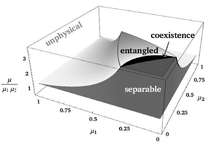
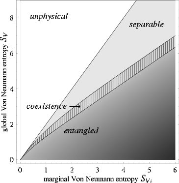
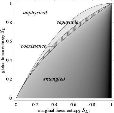
The previous necessary or sufficient conditions for entanglement are collected in Table 1 and allow a graphical display of the behavior of the entanglement of mixed Gaussian states as shown in Fig. 4. These relations classify the properties of separability of all two-mode Gaussian states according to their degree of global and marginal purities.

Degrees of Purity	Separability
$\mu<\mu_{1}\mu_{2}$	unphysical region
$\mu_{1}\mu_{2}\;\leq\;\mu\;\leq\;\frac{\mu_{1}\mu_{2}}{\mu_{1}+\mu_{2}-\mu_{1}\mu_{2}}$	separable states
$\frac{\mu_{1}\mu_{2}}{\mu_{1}+\mu_{2}-\mu_{1}\mu_{2}}<\mu\leq\frac{\mu_{1}\mu_{2}}{\sqrt{\mu_{1}^{2}+\mu_{2}^{2}-\mu_{1}^{2}\mu_{2}^{2}}}$	coexistence region
$\frac{\mu_{1}\mu_{2}}{\sqrt{\mu_{1}^{2}+\mu_{2}^{2}-\mu_{1}^{2}\mu_{2}^{2}}}<\mu\leq\frac{\mu_{1}\mu_{2}}{\mu_{1}\mu_{2}+\left|\mu_{1}-\mu_{2}\right|}$	entangled states
$\mu>\frac{\mu_{1}\mu_{2}}{\mu_{1}\mu_{2}+\left|\mu_{1}-\mu_{2}\right|}$	unphysical region

Table 1: Classification of two–mode Gaussian states and of their properties of separability according to their degrees of global purity $\mu$ and of marginal purities $\mu_{1}$ and $\mu_{2}$.

VII.1 Realization of extremally entangled states in experimental settings

As we have seen, GMEMS are two-mode squeezed thermal states, whose general covariance matrix is described by Eqs. (9) and (15). A realistic instance giving rise to such states is provided by the dissipative evolution of an initially pure two-mode squeezed vacuum created, e.g., in a non degenerate parametric down conversion process. Let us denote by $\boldsymbol{\sigma}_{r}$ the covariance matrix of a two mode squeezed vacuum with squeezing parameter $r$, derived from Eqs. (15) with $\nu_{\mp}=1$. The interaction of this initial state with a thermal noise results in the following dynamical map describing the time evolution of the covariance matrix $\boldsymbol{\sigma}(t)$ dumodi

$$\boldsymbol{\sigma}(t)=\,{\rm e}^{-\Gamma t}\boldsymbol{\sigma}_{r}+(1-\,{\rm e}^{-\Gamma t})\boldsymbol{\sigma}_{n_{1},n_{2}}\;,$$ (71)

where $\Gamma$ is the coupling to the noisy reservoir (equal to the inverse of the damping time) and $\boldsymbol{\sigma}_{n_{1},n_{2}}=\oplus_{i=1}^{2}n_{i}{\mathbbm{1}}_{2}$ is the covariance matrix of the thermal noise. The average number of thermal photons $n_{i}$ given by

$$n_{i}=\frac{1}{\exp\left(\hbar\omega_{i}/k_{B}T\right)-1}$$

in terms of the frequencies of the modes $\omega_{i}$ and of the temperature of the reservoir $T$. It can be easily verified that the covariance matrix Eq. (71) defines a two-mode thermal squeezed state, generally nonsymmetric (for $n_{1}\neq n_{2}$). However, notice that the entanglement of such a state cannot persist indefinetely, becaus after a given time inequality (39) will be violated and the state will evolve into a non entangled two-mode squeezed thermal state. We also notice that the relevant instance of pure loss ($n_{1}=n_{2}=0$) allows the realization of symmetric GMEMS.

Concerning the experimental characterization of minimally entangled states, one can envisage several explicit experimental settings for their realiazion. For instance, let us consider (see Fig. 5) a beam splitter with transmittivity $\tau=1/2$ (corresponding to a two-mode rotation of angle $\pi/4$ in phase space).

Figure 5: Possible scheme for the generation of Gaussian least entangled mixed states (GLEMS). A single-mode squeezed state (obtained, for example, by an optical parametric oscillator or amplifier) interferes with a thermal state through a 50:50 beam splitter. The resulting two-mode state is a minimally entangled mixed Gaussian state at given global and marginal purities.

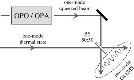
Suppose that a single-mode squeezed state, with covariance matrix $\boldsymbol{\sigma}_{1r}=\,{\rm diag}\,(\,{\rm e}^{2r},\,{\rm e}^{-2r})$ (like, e.g., the result of a degenerate parametric down conversion in a nonlinear crystal), enters in the first input of the beam splitter. Let the other input be an incoherent thermal state produced from a source at equilibrium at a temperature $T$. The purity $\mu$ of such a state can be easily computed in terms of the temperature $T$ and of the frequency of the thermal mode $\omega$

$$\mu=\frac{\exp\left(\hbar\omega/k_{B}T\right)-1}{\exp\left(\hbar\omega/k_{B}T\right)+1}\;.$$ (72)

The state at the output of the beam splitter will be a correlated two-mode Gaussian state with covariance matrix $\boldsymbol{\sigma}_{out}$ that reads

$$\boldsymbol{\sigma}_{out}=\frac{1}{2}\left(\begin{array}[]{cccc}n+k&0&n-k&0\\ 0&n+k^{-1}&0&n-k^{-1}\\ n-k&0&n+k&0\\ 0&n-k^{-1}&0&n+k^{-1}\end{array}\right)\;,$$

with $k=\,{\rm e}^{2r}$ and $n=\mu^{-1}$. By immediate inspection, the symplectic spectrum of this covariance matrix is $\nu_{-}=1$ and $\nu_{+}=1/\mu$. Therefore the output state is always a state with extremal generalized entropy at a given purity (the state can be seen as the tensor product of a vacuum and of a thermal state, on which one has applied symplectic transformation). Moreover, the state is entangled if

$$\cosh(2r)>\frac{\mu^{2}+1}{2\mu}=\frac{\exp\left(2\hbar\omega/k_{B}T\right)+1}{\exp\left(2\hbar\omega/k_{B}T\right)-1}\,.$$ (73)

Tuning the experimental parameters to meet the above condition, indeed makes the output state of the beam splitter a symmetric GLEMS. It is interesting to observe that nonsysmmetric GLEMS can be produced as well by choosing a beam splitter with transmissivity different from $0.5$.

VIII Extremal entanglement at fixed global and local generalized entropies

In this section we introduce a more general characterization of the entanglement of generic two–mode Gaussian states, by exploiting the generalized $p-$entropies as measures of global and marginal mixedness. For ease of comparison we will carry out this analysis along the same lines followed in the previous Section, by studying the explicit behavior of the global invariant $\Delta$, directly related to the logarithmic negativity $E_{\cal N}$ at fixed global and marginal entropies. This study will clarify the relation between $\Delta$ and the generalized entropies $S_{p}$ and the ensuing consequences for the entanglement of Gaussian states.

We begin by observing that the standard form covariance matrix $\boldsymbol{\sigma}$ of a generic two–mode Gaussian state can be parametrized by the following quantities: the two marginals $\mu_{1,2}$ (or any other marginal $S_{p_{1,2}}$ because all the local, single-mode entropies are equivalent for any value of the integer $p$), the global $p-$entropy $S_{p}$ (for some chosen value of the integer $p$), and the global symplectic invariant $\Delta$. On the other hand, Eqs. (18,21,13) provide an explicit expression for any $S_{p}$ as a function of $\mu$ and $\Delta$. Such an expression can be exploited to study the behaviour of $\Delta$ as a function of the global purity $\mu$, at fixed marginals and global $S_{p}$ (from now on we will omit the explicit reference to fixed marginals). One has

$$\left.\frac{\partial\mu}{\partial\Delta}\right|_{S_{p}}=-\frac{2}{R^{2}}\left.\frac{\partial R}{\partial\Delta}\right|_{S_{p}}=\frac{2}{R^{2}}\frac{\left.\partial S_{p}/\partial\Delta\right|_{R}}{\left.\partial S_{p}/\partial R\right|_{\Delta}}$$

$$=\frac{2}{R^{2}}\frac{N_{p}(\Delta,R)}{D_{p}(\Delta,R)}\;,$$ (74)

where we have defined the inverse participation ratio

$$R\equiv\frac{2}{\mu}\;,$$ (75)

and the remaining quantities $N_{p}$ and $D_{p}$ read

$$N_{p}(\Delta,R) = \left[(R+2+2\sqrt{\Delta+R})^{p-1}\right.$$

$$- \left.(R+2-2\sqrt{\Delta+R})^{p-1}\right]\sqrt{\Delta-R}$$

$$- \left[(R-2+2\sqrt{\Delta-R})^{p-1}\right.$$

$$- \left.(R-2-2\sqrt{\Delta-R})^{p-1}\right]\sqrt{\Delta+R}\;,$$

$$D_{p}(\Delta,R) = \left[(\sqrt{\Delta+R}+1)(R+2+2\sqrt{\Delta+R})^{p-1}\right.$$ (76)

$$+ \left.(\sqrt{\Delta+R}-1)(R+2-2\sqrt{\Delta+R})^{p-1}\right]$$

$$\cdot \sqrt{\Delta-R}$$

$$- \left[(\sqrt{\Delta-R}+1)(R-2-2\sqrt{\Delta-R})^{p-1}\right.$$

$$+ \left.(\sqrt{\Delta-R}-1)(R-2+2\sqrt{\Delta-R})^{p-1}\right]$$

$$\cdot \sqrt{\Delta+R}\;.$$

Now, it is easily shown that the ratio $N_{p}(\Delta,R)/D_{p}(\Delta,R)$ is increasing with increasing $p$ and has a zero at $p=2$ for any $\Delta,R$; in particular, its absolute minimum $(-1)$ is reached in the limit $(\Delta\rightarrow 2,\,R\rightarrow 2,\,p\rightarrow 1)$. Thus the derivative Eq. (74) is negative for $p<2$, null for $p=2$ (in this case $\Delta$ and $S_{2}=1-\mu$ are of course regarded as independent variables) and positive for $p>2$. This implies that, for given marginals, keeping fixed any global $S_{p}$ for $p<2$ the minimum (maximum) value of $\Delta$ corresponds to the maximum (minimum) value of the global purity $\mu$. Instead, by keeping fixed any global $S_{p}$ for $p>2$ the minimum of $\Delta$ is always attained at the minimum of the global purity $\mu$.

This observation allows to determine rather straightforwardly the states with extremal $\Delta$. They are extremally entangled states because, for fixed global and marginal entropies, the logarithmic negativity of a state is determined only by the one remaining independent global symplectic invariant, represented by $\Delta$ in our choice of parametrization. If, for the moment being, we neglect the fixed local purities, then the states with maximal $\Delta$ are the states with minimal (maximal) $\mu$ for a given global $S_{p}$ with $p<2\ (p>2)$ (see Sec. III and Fig. 1). As found in Sec. III, such states are minimum uncertainty two–mode states with mixedness concentrated in one quadrature. We have shown in Sec. VII that they correspond to Gaussian least entangled mixed states (GLEMS) whose standard form is given by Eq. (LABEL:glems). As can be seen from Eq. (LABEL:glems), these states are consistent with any legitimate physical value of the local invariants $\mu_{1,2}$. We therefore conclude that all Gaussian states with maximal $\Delta$ for any fixed triple of values of global and marginal entropies are GLEMS.

Viceversa one can show that all Gaussian states with minimal $\Delta$ for any fixed triple of values of global and marginal entropies are Gaussian maximally entangled mixed states (GMEMS). This fact is immediately evident in the symmetric case because the extremal surface in the $S_{p}$ vs. $S_{L}$ diagrams is always represented by symmetric two–mode squeezed states (symmetric GMEMS). These states are characterized by a degenerate symplectic spectrum and encompass only equal choices of the local invariants: $\mu_{1}=\mu_{2}$. In the nonsymmetric case, the given values of the local entropies are different, and the extremal value of $\Delta$ is further constrained by inequality (60)

$$\Delta-R\geq\frac{(\mu_{1}-\mu_{2})^{2}}{\mu_{1}^{2}\mu_{2}^{2}}\;.$$ (77)

From Eq. (74) it follows that

$$\left.\frac{\partial(\Delta-R)}{\partial\Delta}\right|_{S_{p},\mu_{1,2}}=1+\frac{N_{p}(\Delta,R)}{D_{p}(\Delta,R)}\geq 0\,,$$ (78)

because $N_{p}(\Delta,R)/D_{p}(\Delta,R)>-1$. Thus, $\Delta-R$ is an increasing function of $\Delta$ at fixed $\mu_{1,2}$ and $S_{p}$, and the minimal $\Delta$ corresponds to the minimum of $\Delta-R$, which occurs if inequality (77) is saturated. Therefore, also in the nonsymmetric case, the two-mode Gaussian states with minimal $\Delta$ at fixed global and marginal entropies are GMEMS.

Summing up, we have shown that GMEMS and GLEMS introduced in the previous section at fixed global and marginal linear entropies, are always extremally entangled Gaussian states, whatever triple of generalized global and marginal entropic measures one chooses to fix. Maximally and minimally entangled states of CV systems are thus very robust with respect to the choice of different measures of mixedness. This is at striking variance with the case of discrete variable systems, where it has been shown that fixing different measures of mixedness yields different classes of maximally entangled states wei03 .

Furthermore, we will now show that the characterization provided by the generalized entropies leads to some remarkable new insight on the behavior of the entanglement of CV systems. The crucial observation is that for a generic $p$, the smallest symplectic eigenvalue of the partially transposed covariance matrix, at fixed global and marginal $p-$entropies, is not in general a monotone function of $\Delta$, so that the connection between extremal $\Delta$ and extremal entanglement turns out to be, in some cases, inverted. In particular, while for $p<2$ the GMEMS and GLEMS surfaces tend to be more separated as $p$ decreases, for $p>2$ the two classes of extremally entangled states get closer with increasing $p$ and, within a particular range of global and marginal entropies, they exchange their role. GMEMS (i.e. states with minimal $\Delta$) become minimally entangled states and GLEMS (i.e. states with maximal $\Delta$) become maximally entangled states. This inversion always occurs for all $p>2$.

To understand this interesting behaviour, let us study the dependence of the symplectic eigenvalue $\tilde{\nu}_{-}$ on the global invariant $\Delta$ at fixed marginals and at fixed $S_{p}$ for a generic $p$. Using Maxwell’s relations, we can write

$$\kappa_{p}\equiv\left.\frac{\partial(2\tilde{\nu}_{-}^{2})}{\partial\Delta}\right|_{S_{p}}=\left.\frac{\partial(2\tilde{\nu}_{-}^{2})}{\partial\Delta}\right|_{R}-\left.\frac{\partial(2\tilde{\nu}_{-}^{2})}{\partial R}\right|_{\Delta}\cdot\frac{\left.\partial S_{p}/\partial\Delta\right|_{R}}{\left.\partial S_{p}/\partial R\right|_{\Delta}}\,.$$ (79)

Clearly, for $\kappa_{p}>0$ GMEMS and GLEMS retain their usual interpretation, whereas for $\kappa_{p}<0$ they exchange their role. On the node $\kappa_{p}=0$ GMEMS and GLEMS share the same entanglement, i.e. the entanglement of all Gaussian states at $\kappa_{p}=0$ is fully determined by the global and marginal $p-$entropies alone, and does not depend any more on $\Delta$. Such nodes also exist in the case $p\leq 2$ in two limiting instances: in the special case of GMEMMS (states with maximal global purity at fixed marginals) and in the limit of zero marginal purities. We will now show that, besides these two limiting behaviors, a nontrivial node appears for all $p>2$, implying that on the two sides of the node GMEMS and GLEMS indeed exhibit opposite behaviors. Because of Eq. (74), $\kappa_{p}$ can be written in the following form

$$\kappa_{p}=\kappa_{2}-\frac{R}{\sqrt{\tilde{\Delta}^{2}-R^{2}}}\,\frac{N_{p}(\Delta,R)}{D_{p}(\Delta,R)}\;,$$ (80)

with $N_{p}$ and $D_{p}$ defined by Eq. (76) and

$$\tilde{\Delta} = -\Delta+\frac{2}{\mu_{1}^{2}}+\frac{2}{\mu_{2}^{2}}\;,$$

$$\kappa_{2} = -1+\frac{\tilde{\Delta}}{\sqrt{\tilde{\Delta}^{2}-R^{2}}}\;,$$

Figure 6: Plot of the nodal surface which solves the equation $\kappa_{p}=0$ with $\kappa_{p}$ defined by Eq. (80), for (a) $p=3$ and (b) $p=4$. The entanglement of Gaussian states that lie on the leaf–shaped surfaces is fully quantified in terms of the marginal purities and the global generalized entropy (a) $S_{3}$ or (b) $S_{4}$. The equations of the surfaces in the space $\mathcal{E}_{p}\equiv\{\mu_{1},\mu_{2},S_{p}\}$ are given by Eqs. (83–LABEL:spleaf4).

The quantity $\kappa_{p}$ in Eq. (80) is a function of $p,\,R,\,\Delta,\,$ and of the marginals; since we are looking for the node (where the entanglement is independent of $\Delta$), we can investigate the existence of a nontrivial solution to the equation $\kappa_{p}=0$ fixing any value of $\Delta$. Let us choose $\Delta=1+R^{2}/4$ that saturates the Heisenberg uncertainty relation and is satisfied by GLEMS. With this position, Eq. (80) becomes

$$\kappa_{p}(\mu_{1},\mu_{2},R) = \kappa_{2}(\mu_{1},\mu_{2},R)$$

$$- \frac{R}{\sqrt{\left(\frac{2}{\mu_{1}^{2}}+\frac{2}{\mu_{2}^{2}}-\frac{R^{2}}{4}-1\right)^{2}-R^{2}}}\,f_{p}(R)\,.$$

The existence of the node depends then on the behavior of the function

$$f_{p}(R)\equiv\frac{2\left[(R+2)^{p-2}-(R-2)^{p-2}\right]}{(R+4)(R+2)^{p-2}-(R-4)(R-2)^{p-2}}\;.$$ (82)

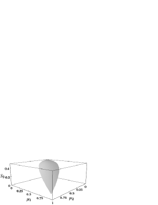
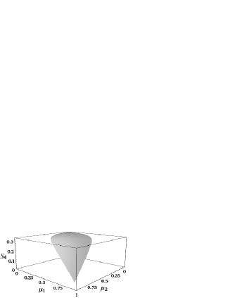
In fact, as we have already pointed out, $\kappa_{2}$ is always positive, while the function $f_{p}(R)$ is an increasing function of $p$ and, in particular, it is negative for $p<2$, null for $p=2$ and positive for $p>2$, reaching its asymptote $2/(R+4)$ in the limit $p\rightarrow\infty$. This entails that, for $p\leq 2$, $\kappa_{p}$ is always positive, which in turn implies that GMEMS and GLEMS are respectively maximally and minimally entangled two–mode states with fixed marginal and global $p-$entropies in the range $p\leq 2$ (including both von Neumann and linear entropies). On the other hand, for any $p>2$ one node can be found solving the equation $\kappa_{p}(\mu_{1},\mu_{2},2/\mu)=0$. The solutions to this equation can be found analytically for low $p$ and numerically for any $p$. They form a continuum in the space $\{\mu_{1},\mu_{2},\mu\}$ which can be expressed as a surface of general equation $\mu=\mu^{\kappa}_{p}(\mu_{1},\mu_{2})$. Since the fixed variable is $S_{p}$ and not $\mu$ it is convenient to rewrite the equation of this surface in the space $\mathcal{E}_{p}\equiv\{\mu_{1},\mu_{2},S_{p}\}$, keeping in mind the relation (34), holding for GLEMS, between $\mu$ and $S_{p}$. In this way the nodal surface $(\kappa_{p}=0)$ can be written in the form

$$S_{p}=S_{p}^{\kappa}(\mu_{1},\mu_{2})\equiv\frac{1-g_{p}\left[(\mu_{p}^{\kappa}(\mu_{1},\mu_{2}))^{-1}\right]}{p-1}\;.$$ (83)

The entanglement of all Gaussian states whose entropies lie on the surface $S_{p}^{\kappa}(\mu_{1},\mu_{2})$ is completely determinated by the knowledge of $\mu_{1}$, $\mu_{2}$ and $S_{p}$. The explicit expression of the function $\mu^{\kappa}_{p}(\mu_{1},\mu_{2})$ depends on $p$ but, being the global purity of physical states, is constrained by the inequality

$$\mu_{1}\mu_{2}\,\leq\,\mu^{\kappa}_{p}(\mu_{1},\mu_{2})\,\leq\,\frac{\mu_{1}\mu_{2}}{\mu_{1}\mu_{2}+\left|\mu_{1}-\mu_{2}\right|}\;.$$

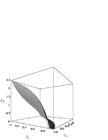
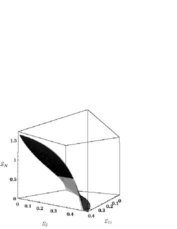
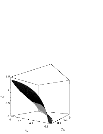
The nodal surface of Eq. (83) constitutes a ‘leaf’, with base at the point $\mu^{\kappa}_{p}(0,0)=0$ and tip at the point $\mu^{\kappa}_{p}(\sqrt{3}/2,\sqrt{3}/2)=1$, for any $p>2$; such a leaf becomes larger and flatter with increasing $p$ (see Fig. 6). For $p>2$, the function $f_{p}(R)$ defined by Eq. (82) is negative but decreasing with increasing $R$, that is with decreasing $\mu$. This means that, in the space of entropies $\mathcal{E}_{p}$, above the leaf $(S_{p}>S_{p}^{\kappa})$ GMEMS (GLEMS) are still maximally (minimally) entangled states for fixed global and marginal generalized entropies, while below the leaf they are inverted. Notice also that for $\mu_{1,2}>\sqrt{3}/2$ no node and so no inversion can occur for any $p$. Each point on the leaf–shaped surface of Eq. (83) corresponds to an entire class of infinitely many two–mode Gaussian states (including GMEMS and GLEMS) with the same marginals and the same global $S_{p}=S_{p}^{\kappa}(\mu_{1},\mu_{2})$, which are all equally entangled, since their logarithmic negativity is completely determined by $\mu_{1},\mu_{2}$ and $S_{p}$. For the sake of clarity we provide the explicit expressions of $\mu_{p}^{\kappa}(\mu_{1},\mu_{2})$, as plotted in Fig. 6 for the cases (a) $p=3$, and (b) $p=4$.

$$\mu_{3}^{\kappa}(\mu_{1},\mu_{2}) = \left(\frac{6}{\frac{3}{\mu_{1}^{2}}+\frac{3}{\mu_{1}^{2}}-2}\right)^{\frac{1}{2}},$$ (84)

$$\mu_{4}^{\kappa}(\mu_{1},\mu_{2}) = \sqrt{3}\,\mu_{1}\mu_{2}\,\,\,\bigg{/}\,\,\,\bigg{(}\mu_{1}^{2}+\mu_{2}^{2}-2\mu_{1}^{2}\mu_{2}^{2}+$$

$$\sqrt{\left(\mu_{1}^{2}+\mu_{2}^{2}\right)\left(\mu_{1}^{2}+\mu_{2}^{2}-\mu_{1}^{2}\mu_{2}^{2}\right)+\mu_{1}^{4}\mu_{2}^{4}}\bigg{)}^{\frac{1}{2}}.$$

(a)

(b)

(c)

(d)

Figure 7: Summary of the entanglement properties for symmetric Gaussian states at fixed global and marginal generalized $p-$entropies, for (a) $p=1$ (von Neumann entropies), (b) $p=2$ (linear entropies), (c) $p=3$, and (d) $p=4$. In the entangled region, the average logarithmic negativity $\bar{E}_{{\cal N}}(S_{p_{i}},S_{p})$ Eq. (88) is depicted, growing from gray to black. For $p>2$ an additional dashed curve is plotted; it represents the nodal line of inversion. Along it the entanglement is fully determined by the knowledge of the global and marginal generalized entropies $S_{p_{i}},S_{p}$, and GMEMS and GLEMS are equally entangled. On the left side of the nodal line GMEMS (GLEMS) are maximally (minimally) entangled Gaussian states at fixed $S_{p_{i}},S_{p}$. On the right side of the nodal line they are inverted: GMEMS (GLEMS) are minimally (maximally) entangled states. Also notice how the dashed region of coexistence becomes narrower with increasing $p$. The equations of all boundary curves can be found in Eq. (86).

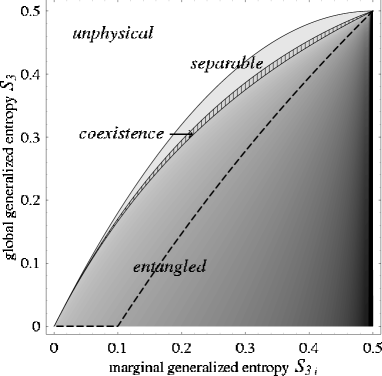
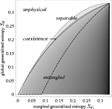
Apart from the relevant ‘inversion’ feature shown by $p-$entropies for $p>2$, the possibility of an accurate characterization of CV entanglement based on global and marginal entropic measures still holds in the general case for any $p$. In particular, the set of all Gaussian states can be again divided, in the space of global and marginal $S_{p}$’s, into three main areas: separable, entangled and coexistence region. It can be thus very interesting to investigate how the different entropic measures chosen to quantify the degree of global mixedness (all marginal measures are equivalent) behave in classifying the separability properties of Gaussian states. Fig. 7 provides a numerical comparison of the different characterizations of entanglement obtained by the use of different $p-$entropies, with $p$ ranging from $1$ to $4$, for symmetric Gaussian states ($S_{p_{1}}=S_{p_{2}}\equiv S_{p_{i}}$). The last restriction has been imposed just for ease of graphical display. The following considerations, based on the exact numerical solutions of the transcendental conditions, will take into account nonsymmetric states as well.

The mathematical relations expressing the boundaries between the different regions in Fig. 7 are easily obtained for any $p$ by starting from the relations holding for $p=2$ (see Table 1) and by evaluating the corresponding $S_{p}(\mu_{1,2})$ for each $\mu(\mu_{1,2})$. For any physical symmetric state such a calculation yields

$$0\leq(p-1)S_{p} \!\!<\!\! 1-g_{p}\left(\frac{\sqrt{2-\mu_{i}^{2}}}{\mu_{i}}\right)$$

$$\Rightarrow$$ entangled,

$$1-g_{p}\left(\frac{\sqrt{2-\mu_{i}^{2}}}{\mu_{i}}\right)\leq(p-1)S_{p} \!\!<\!\! 1-g_{p}^{2}\left(\sqrt{\frac{2-\mu_{i}}{\mu_{i}}}\right)$$

$$\Rightarrow$$ coexistence,

$$1-g_{p}^{2}\left(\sqrt{\frac{2-\mu_{i}}{\mu_{i}}}\right)\leq(p-1)S_{p} \!\!\leq\!\! 1-g_{p}^{2}\left(\frac{1}{\mu_{i}^{2}}\right)$$ (86)

$$\Rightarrow$$ separable.

Equations (86) were obtained exploiting the multiplicativity of $p-$norms on product states and using Eq. (27) for the lower boundary of the coexistence region (which represents GLEMS becoming entangled) and Eq. (30) for the upper one (which expresses GMEMS becoming separable). Let us mention also that the relation between any local entropic measure $S_{p_{i}}$ and the local purity $\mu_{i}$ is obtained directly from Eq. (21) and reads

$$S_{p_{i}}=\frac{1-g_{p}(1/\mu_{i})}{p-1}\,.$$ (87)

We notice prima facie that, with increasing $p$, the entanglement is more sharply qualified in terms of the global and marginal $p-$entropies. In fact the region of coexistence between separable and entangled states becomes narrower with higher $p$. Thus, somehow paradoxically, with increasing $p$ the entropy $S_{p}$ provides less information about a quantum state, but at the same time it yields a more accurate characterization and quantification of its entanglement. In the limit $p\rightarrow\infty$ all the physical states collapse to one point at the origin of the axes in the space of generalized entropies, due to the fact that the measure $S_{\infty}$ is identically zero.

(a)

(b)

(c)

(d)

Figure 8: Upper and lower bounds on the logarithmic negativity of symmetric Gaussian states as functions of the global and marginal generalized $p-$entropies, for (a) $p=1$ (von Neumann entropies), (b) $p=2$ (linear entropies), (c) $p=3$, and (d) $p=4$. The black (gray) surface represents GMEMS (GLEMS). Notice that for $p>2$ GMEMS and GLEMS surfaces intersect along the inversion line (meaning they are equally entangled along that line), and beyond it they interchange their role. The equations of the inversion lines are obtained from Eqs. (83–LABEL:spleaf4), with the position $S_{p_{1}}=S_{p_{2}}\equiv S_{p_{i}}$.

IX Quantifying Entanglement: the average logarithmic negativity

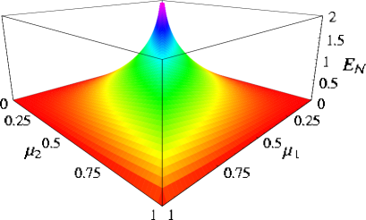
We have extensively shown that knowledge of the global and marginal generalized $p-$entropies accurately characterizes the entanglement of Gaussian states, providing strong sufficient or necessary conditions. The present analysis naturally leads us to propose an actual quantification of entanglement, based exclusively on marginal and global entropic measures, enriching and generalizing the approach introduced in Ref. adeser04 .

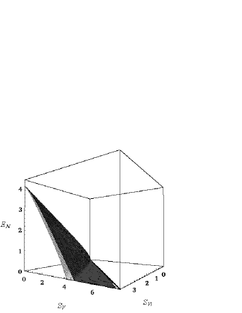
Outside the separable region, we can formally define the maximal entanglement $E_{{{\cal N}}max}(S_{p_{1,2}},S_{p})$ as the logarithmic negativity attained by GMEMS (or GLEMS, below the inversion nodal surface for $p>2$, see Fig. 6). In a similar way, in the entangled region GLEMS (or GMEMS, below the inversion nodal surface for $p>2$) achieve the minimal logarithmic negativity $E_{{{\cal N}}max}(S_{p_{1,2}},S_{p})$. The explicit analytical expressions of these quantities are unavailable for any $p\neq 2$ due to the transcendence of the conditions relating $S_{p}$ to the symplectic eigenvalues. The surfaces of maximal and minimal entanglement in the space of the global and local $S_{p}$ are plotted in Fig. 8 for symmetric states. In the plane $S_{p}=0$ the upper and lower bounds correctly coincide, since for pure states the entanglement is completely quantified by the marginal entropy. For mixed states this is not the case but, as the plot shows, knowledge of the global and marginal entropies strictly bounds the entanglement both from above and from below. For $p>2$, we notice how GMEMS and GLEMS exchange their role beyond a specific curve in the space of $S_{p}$’s. The equation of this nodal curve is obtained from the general leaf–shaped nodal surfaces of Eqs. (83–LABEL:spleaf4), by imposing the symmetry constraint ($S_{p_{1}}=S_{p_{2}}\equiv S_{p_{i}}$). We notice again how the $S_{p}$’s with higher $p$ provide a better characterization of the entanglement, even quantitatively. In fact, the gap between the two extremally entangled surfaces in the $S_{p}$’s space becomes smaller with higher $p$. Of course the gap is exactly zero all along the nodal line of inversion for $p>2$.

(a)

(b)

(c)

(d)

Figure 9: The relative error $\delta\bar{E}_{{\cal N}}$ Eq. (89) on the average logarithmic negativity as a function of the ratio $S_{p_{i}}/S_{p}$, for (a) $p=1$, (b) $p=2$, (c) $p=3$, (d) $p=4$, plotted at (a) $S_{V}=1$, (b) $S_{L}=1/2$, (c) $S_{3}=1/4$, (d) $S_{4}=1/6$. Notice how, in general, the error decays exponentially, and in particular faster with increasing $p$. For $p>2$, notice how the error reaches zero on the inversion node (see the insets), then grows and reaches a local maximum before going back to zero asymptotically.

We will now introduce a particularly convenient quantitative estimate of the entanglement based only on the knowledge of the global and marginal entropies. Let us define the “average logarithmic negativity” $\bar{E}_{{\cal N}}$ as

$$\bar{E}_{{\cal N}}(S_{p_{1,2}},S_{p})\equiv\frac{E_{{{\cal N}}max}(S_{p_{1,2}},S_{p})+E_{{{\cal N}}min}(S_{p_{1,2}},S_{p})}{2}\;.$$ (88)

We will now show that this quantity, fully determined by the global and marginal entropies, provides a reliable quantification of entanglement (logarithmic negativity) for two–mode Gaussian states. To this aim, we define the relative error $\delta\bar{E}_{{\cal N}}$ on $\bar{E}_{{\cal N}}$ as

$$\delta\bar{E}_{{\cal N}}(S_{p_{1,2}},S_{p})\equiv\frac{E_{Nmax}(S_{p_{1,2}},S_{p})-E_{Nmin}(S_{p_{1,2}},S_{p})}{E_{Nmax}(S_{p_{1,2}},S_{p})+E_{Nmin}(S_{p_{1,2}},S_{p})}\,.$$ (89)

As Fig. 9 shows, this error decreases exponentially both with decreasing global entropy and increasing marginal entropies, that is with increasing entanglement. In general the relative error $\delta\bar{E}_{{\cal N}}$ is ‘small’ for sufficiently entangled states; we will present more precise numerical considerations in the subcase $p=2$. Notice that the decaying rate of the relative error is faster with increasing $p$: the average logarithmic negativity turns out to be a better estimate of entanglement with increasing $p$. For $p>2$, $\delta\bar{E}_{{\cal N}}$ is exactly zero on the inversion node, then it becomes finite again and, after reaching a local maximum, it goes asymptotically to zero (see the insets of Fig. 9).

All the above considerations, obtained by an exact numerical analysis, show that the average logarithmic negativity $\bar{E}_{{\cal N}}$ at fixed global and marginal $p-$entropies is a very good estimate of entanglement in CV systems, whose reliability improves with increasing entanglement and, surprisingly, with increasing order $p$ of the entropic measures.

IX.1 Direct estimate of the entanglement

In the present general framework, a peculiar role is played by the case $p=2$, i.e. by the linear entropy $S_{L}$ (or, equivalently, the purity $\mu$). The previous general analysis on the whole range of generalized entropies $S_{p}$, has remarkably stressed the privileged theoretical role of the instance $p=2$, which discriminates between the region in which extremally entangled states are unambiguously characterized and the region in which they can exchange their roles. Moreover, the graphical analysis shows that, in the region where no inversion takes place $(p\leq 2)$, fixing the global $S_{2}=1-\mu$ yields the most stringent constraints on the logarithmic negativity of the states (see Figs. 7, 8, 9). Notice that such constraints, involving no transcendental functions for $p=2$, can be easily handled analytically. A crucial experimental consideration strengthens these theoretical and practical reasons to privilege the role of $S_{2}$. In fact, $S_{2}$ can indeed, assuming some prior knowledge about the state (essentially, its Gaussian character), be measured through conceivable direct methods, in particular by means of single–photon detection schemes fiurcerf03 or of the upcoming quantum network architectures network . No complete homodyne reconstruction of the density matrix is needed in such schemes. Very recently, a first important and promising step in this direction has been realized with the experimental implementation of direct photon detection for the measurement of the squeezing and purity of a single-mode squeezed vacuum with a setup that required only a tunable beam splitter and a single-photon detector wenger .

As already anticipated, for $p=2$ we can provide analytical expressions for the extremal entanglement in the space of global and marginal purities

$$E_{{{\cal N}}max}(\mu_{1,2},\mu)=-\frac{1}{2}\log\Bigg{[}-\frac{1}{\mu}+\left(\frac{\mu_{1}+\mu_{2}}{2\mu_{1}^{2}\mu_{2}^{2}}\right)$$

$$\times\left(\mu_{1}+\mu_{2}-\sqrt{(\mu_{1}+\mu_{2})^{2}-\frac{4\mu_{1}^{2}\mu_{2}^{2}}{\mu}}\right)\Bigg{]}\,,$$ (90)

$$E_{{{\cal N}}min}(\mu_{1,2},\mu)=-\frac{1}{2}\log\Bigg{[}\frac{1}{\mu_{1}^{2}}+\frac{1}{\mu_{2}^{2}}-\frac{1}{2\mu^{2}}-\frac{1}{2}$$

$$-\sqrt{\left(\frac{1}{\mu_{1}^{2}}+\frac{1}{\mu_{2}^{2}}-\frac{1}{2\mu^{2}}-\frac{1}{2}\right)^{2}-\frac{1}{\mu^{2}}}\;\Bigg{]}\,.$$ (91)

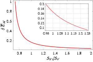
Consequently, both the average logarithmic negativity $\delta\bar{E}_{{\cal N}}$, defined in Eq. (88), and the relative error $\delta\bar{E}_{{\cal N}}$, given by Eq. (89), can be easily evaluated in terms of the purities. The relative error is plotted in Fig. 9(b) for symmetric states as a function of the ratio $S_{L_{i}}/S_{L}$. Notice, as already pointed out in the general instance of arbitrary $p$, how the error decays exponentially. In particular, it falls below $5\%$ in the range $S_{L}<S_{L_{i}}\ (\mu>\mu_{i})$, which excludes at most very weakly entangled states (states with $E_{{\cal N}}\lesssim 1$ sqpar ). Let us remark that the accuracy of estimating entanglement by the average logarithmic negativity proves even better in the nonsymmetric case $\mu_{1}\neq\mu_{2}$, essentially because the maximal allowed entanglement decreases with the difference between the marginals, as shown in Fig. (3)

The above analysis proves that the average logarithmic negativity $\bar{E}_{{\cal N}}$ is a reliable estimate of the logarithmic negativity $E_{{\cal N}}$, improving as the entanglement increases. This allows for an accurate quantification of continuous variable entanglement by knowledge of the global and marginal purities. As we already mentioned, the latter quantities may be in turn amenable to direct experimental determination by exploiting recent single–photon detection proposals or the upcoming technology of quantum networks.

X Summary and concluding remarks

Summarizing, we have pointed out the existence of both maximally and minimally entangled two–mode Gaussian states at fixed local and global generalized $p-$entropies. The analytical properties of such states have been studied in detail for any value of $p$. Remarkably, for $p\leq 2$, minimally entangled states are minimum uncertainty states, saturating the Heisenberg principle, while maximally entangled states are nonsymmetric two–mode squeezed thermal states. Interestingly, for $p>2$ and in specific ranges of the values of the entropic measures, the role of such states is reversed. In particular, for such quantifications of the global and local entropies, two–mode squeezed thermal states, often referred to as continuous variable analog of maximally entangled states, turn out to be minimally entangled.

In the search for the extremally entangled states, we focused on the hierarchy of mixedness induced by $p-$entropies on the set of arbitrary multi–mode states, investigating several related subjects, like the ordering of such different entropic measures and the analytical comparison between the generic $S_{p}$ (and in particular the von Neumann entropy $S_{V}$) and the linear entropy $S_{L}$. Moreover, we have introduced the notion of “average logarithmic negativity” for given global and marginal generalized $p$-entropies, showing that it provides a reliable estimate of CV entanglement in a wide range of physical parameters.

Our analysis also clarifies the reasons why the linear entropy is a ‘privileged’ measure of mixedness in continuous variable systems. It is naturally normalized between $0$ and $1$, it offers an accurate qualification and quantification of entanglement of any mixed state while giving significative information about the state itself and, crucially, is the only entropic measure which could be directly measured in the near future by schemes involving only single-photon detections or the technology of quantum networks, without requiring a full homodyne reconstruction of the state.

More generally, the present analysis shows that some of the canonical measures of entanglement and mixedness in the discrete variable scenario, such as the entanglement of formation and the von Neumann entropy, may not be the best choices for the characterization of mixed states of continuous variable systems. Discontinuous behaviors appear in the limit of infinite dimensions for quantities like the entanglement of formation, even when restricted to the special class of Gaussian states. Entanglement measures such as the logarithmic negativity, and informational measures such as the linear entropy and the generalized entropies of higher order provide quantifications which are, in many respects, more satisfactory (both mathematically and physically) in the context of CV systems.