Gaussian relative entropy of entanglement

Abstract

For two gaussian states with given correlation matrices, in order that relative entropy between them is practically calculable, I in this paper describe the ways of transforming the correlation matrix to matrix in the exponential density operator. Gaussian relative entropy of entanglement is proposed as the minimal relative entropy of the gaussian state with respect to separable gaussian state set. I prove that gaussian relative entropy of entanglement achieves when the separable gaussian state is at the border of separable gaussian state set and inseparable gaussian state set. For two mode gaussian states, the calculation of gaussian relative entropy of entanglement is greatly simplified from searching for a matrix with 10 undetermined parameters to 3 variables. The two mode gaussian states are classified as four types, numerical evidence strongly suggests that gaussian relative entropy of entanglement for each type is realized by the separable state within the same type.For symmetric gaussian state it is strictly proved that it is achieved by symmetric gaussian state.

PACS number:03.67.Mn, 03.65.Ud

1 Introduction

Quantum relative entropy function has many applications in the problems of classical and quantum information transfer and quantum data compression [1]. The relative entropy has a natural interpretation in terms of the statistical distinguishability of quantum states; closely related to this is the picture of relative entropy as a distance measure between density operators. Based on the relative entropy, a nature measure of entanglement called the relative entropy of entanglement was proposed. This entanglement measure is intimately related to the entanglement of distillation by providing an upper bound for it.  It tells us that the amount of entanglement in the state with its distance from the disentangled set of states. In statistical terms, the more entangled a state is the more it is distinguishable from a disentangled state[2]. However, except for some special situations[3], such an entanglement measure is usually very difficult to be calculated for mixed state. For continuous variable system, it is shown that the relative entropy of entanglement is actually trace-norm continuous and hence well-defined even in this infinite-dimensional context[4]. Due to the fact that gaussian state has the merit that the logarithmic of the state operator is in the quadrature form of canonical operators, the distance of the gaussian state to gaussian state measured by the relative entropy (gaussian relative entropy or GRE) was considered [5]. In which the second gaussian state was specified by its exponential operator matrix (EM), not by the usual correlation matrix (CM). Until now, an explicit transform from the CM to EM has not been available, make the calculation of the relative entropy between gaussian states in fact impossible. Moreover, when using the gaussian relative entropy as entanglement measure, the second state should be separable. Now all the separable criterions are not in the form of EM. So the problems of separable criterion in the form of EM or the explicit transform of CM to EM need to be addressed. In this paper, I will give the explicit transform of CM to EM, propose the gaussian relative entropy of entanglement (GREE) and give the method of how to calculate it. The paper is organized as follow: In section 2, the transform of CM to EM for $q-p$ decorrelation gaussian state is given with the help of symplectic transformation, further more, the direct transforms of any CM to EM and EM to CM are also solved due to the commutation relation of matrices. Section 3 deals with GREE with emphasis on the proof of theorem 2 which states that GREE will achieve by gaussian state at border of separable and inseparable gaussian state sets. In section 4, I concentrate on the simplification of GREE for two mode ($1\times 1$) gaussian state system. In section 5, the $1\times 1$ gaussian states are classified as four types, their GREEs are discussed. In section 6, conclusions and discussions are addressed.

2 Matrix in the exponential density operator

To characterize a gaussian state, we have several equivalent means, among them are: quantum characteristic function specified by first (irrelative to the entanglement problem) and second moments which are also called means and CM, density operator in exponential form specified by a matrix M (exponential operator matrix or EM), density operator in exponential form of ordered operators specified by another matrix (ordered exponential operator matrix or OEM). The separability of a gaussian state was obtained with CM [6][7][8], also with OEM [9]. The transform of CM to OEM and vice versa are quite directly by the integral within ordered product of operators. The transform of EM to OEM is also available but involved with a calculation of exponential of matrix[10]. Scheel [5] derived a relation of EM and CM of gaussian state with generation and annihilation operators. Following the way I now derive their relation with canonical operators.

Gaussian quantum state can be given by the density operator

$$\rho=\frac{\exp[-\frac{1}{2}F^{T}MF]}{Tr\{\exp[-\frac{1}{2}F^{T}MF]\}},$$ (1)

where $M$ is a real symmetric matrix, and $F=\left[q_{1},\cdots q_{n};p_{1},\cdots p_{n}\right]^{T}$ , with $q_{j},p_{j}$ are the canonical operators. In order to relate the matrix $M$ to the correlation matrix (CM) $\alpha$, a unitary transformation

$$F^{{}^{\prime}}=UFU^{-1}=SF$$ (2)

is needed. The matrix $S$ produces a symplectic transformation on the canonical operators $F$. To preserve the commutation relations of the canonical operators, $S$ should satisfy the symplectic condition $S\Delta S^{T}=\Delta$. Where

$$\Delta=\left[\begin{array}[]{cc}0&I_{n}\\ -I_{n}&0\end{array}\right].$$ (3)

The matrix $S$ is chosen such that it diagonalizes $M$ , hence $S^{T}MS=$ $\widetilde{M}$ (with $\widetilde{M}$ being diagonal). Then the characteristic function of the density operator (1) is

$$Tr[\rho\exp(iF^{T}z)] = Tr[U\rho U^{-1}U\exp(iF^{T}z)U]$$

$$= \exp[-\frac{1}{2}z^{T}S(\frac{1}{2}\coth\frac{1}{2}\widetilde{M})S^{T}z],$$

and the CM is $\alpha=S(\frac{1}{2}\coth\frac{1}{2}\widetilde{M})S^{T}=S\widetilde{\alpha}S^{T}$. In the derivation the expression for characteristic function of a thermal state has been used.

For a given CM, how to find such a sympleptic transformation is the topics of this section. To find the $S$ matrix, let us consider $\Delta^{-1}\alpha$ instead of $\alpha$, then

$$S^{T}\Delta^{-1}\alpha(S^{T})^{-1}=\Delta^{-1}\widetilde{\alpha}.$$ (5)

The eigenvalues of $\Delta^{-1}\alpha$ come in pairs $\pm i\gamma_{j}$, the matrix uncertainty relation requires $\gamma_{j}\geq\frac{1}{2}$ [13], where $\gamma_{j}$ are called symplectic eigenvalues of $\alpha$ [14], then $\widetilde{\alpha}=diag\{\gamma_{1},\cdots,\gamma_{n},\gamma_{1},\cdots,\gamma_{n}\}$, and $\widetilde{M}=diag\{\widetilde{M}_{1},\cdots,\widetilde{M}_{n},$ $\widetilde{M}_{1},\cdots,\widetilde{M}_{n}\}$, with $\widetilde{M}_{j}=\log\frac{2\gamma_{j}+1}{2\gamma_{j}-1}$ are symplectic eigenvalues of $M$. Let $\widetilde{\Psi}$ be the eigenvector of $\Delta^{-1}\widetilde{\alpha}$ and $\Psi$ be the eigenvector of $\Delta^{-1}\alpha$, then

$$\Psi=(S^{T})^{-1}\widetilde{\Psi}.$$ (6)

So that $S$ matrix can obtained from the eigenvectors. The $S$ matrix so obtained is not totally determined, yet the symplectic condition $S\Delta S^{T}=\Delta$ should be verified.

If the CM is in its $q-p$ decorrelation form, that is $\alpha=\alpha_{q}\oplus\alpha_{p}$, then the details of $S$ can be further worked out. The $q-p$ decorrelation CMs are quite general in concerning with entanglement for $1\times 1$ gaussian states. For these states, the CMs can always be transformed into the form of $\alpha_{q}\oplus\alpha_{p}$ by local operations[6] [7]. For multi-mode bipartite gaussian state, It is not known if the CM can be transformed to the form of $\alpha_{q}\oplus\alpha_{p}$ or not just by local operations. Let us start with the CM of the form $\alpha_{q}\oplus\alpha_{p}$, that is to say the correlation between position and momentum of each mode and inter-modes have already dissolved, so that one just considers a symplectic transformation of form $S=S_{q}\oplus S_{p}$. The relation $S\Delta S^{T}=\Delta$ then will requires that $S_{q}S_{p}^{T}=S_{p}S_{q}^{T}=I$. And $S$ will take the form of $S=S_{q}\oplus(S_{q}^{T})^{-1}$, and $(S^{T})^{-1}=(S_{q}^{T})^{-1}\oplus S_{q}$. $S^{-1}\alpha(S^{T})^{-1}=[S_{q}^{-1}\alpha_{q}(S_{q}^{T})^{-1}]\oplus[S_{q}^{T}\alpha_{p}S_{q}]=\widetilde{\alpha}$. Let $\Psi^{T}=(\Psi_{q}^{T},\Psi_{p}^{T})$ and $\widetilde{\Psi}^{T}=(\widetilde{\Psi}_{q}^{T},\widetilde{\Psi}_{p}^{T})$, then the eigenequation $\Delta^{-1}\alpha\Psi=\pm i\gamma\Psi$ (where $\gamma$ is one of the symplectic eigenvalues of $\alpha$) will be  $-\alpha_{p}\Psi_{p}=\pm i\gamma\Psi_{q}$ and $\alpha_{q}\Psi_{q}=\pm i\gamma\Psi_{p}$. And one gets

$$\alpha_{p}\alpha_{q}\Psi_{q}=\gamma^{2}\Psi_{q}\text{, \ \ \ }\alpha_{q}\alpha_{p}\Psi_{p}=\gamma^{2}\Psi_{p}.$$ (7)

For the eigenvalue $i\gamma_{j}$, suppose the eigenvector of the $q$ part be $\Psi_{qj}^{T}=[c_{j1,}\cdots,c_{jn}].$ Since $\alpha_{p}\alpha_{q}\Psi_{q}^{\ast}=\gamma^{2}\Psi_{q}^{\ast},$ the eigenvector $\Psi_{q}$ can always be chosen to be real. Then $\Psi_{pj}^{T}=-i[c_{j1,}\cdots,c_{jn}]\alpha_{q}/\gamma_{j}$. The similar equation for  $\widetilde{\Psi}$ will at last give the result of

$$\widetilde{\Psi}_{j}^{T}=\frac{1}{\sqrt{2}}\left[0,\cdots,0,1,0,\cdots,0;0,\cdots,0,-i,0,\cdots,0\right]\text{ \ \ for eigenvalue }i\gamma_{j},$$ (8)

where the nonzero elements in the eigenvectors are at the positions of $j$ and $n+j$. By Eq.(6) one gets $\widetilde{\Psi}^{T}(S^{T})^{-1}\widetilde{\Psi}=\widetilde{\Psi}^{T}\Psi$ and $\widetilde{\Psi}^{+}(S^{T})^{-1}\widetilde{\Psi}=\widetilde{\Psi}^{+}\Psi$, then

$$(S_{q}^{T})_{kj}^{-1} = c_{jk}$$ (9)

$$(S_{q})_{kj} = \sum_{l}c_{jl}(\alpha_{q})_{lk}/\gamma_{j}.$$ (10)

One has to verify the consistence of Eq.(9) and Eq.(10), that is $S_{q}^{-1}S_{q}=I_{n}$. The vector $\Psi_{qj}$ has yet a phase factor and its length left to be determined. To determine the phase factor of $\Psi_{qj},$ one simply chooses $c_{jj}$ to be positive. The length of the vector $\Psi_{qj}$ can be chosen such that

$$\sum_{kl}c_{jk}c_{jl}(\alpha_{q})_{lk}/\gamma_{j}=1.$$ (11)

So $\sum_{k}\left(S_{q}^{-1}\right)_{jk}\left(S_{q}\right)_{kj}=1.$ While in proving $\sum_{k}\left(S_{q}^{-1}\right)_{mk}\left(S_{q}\right)_{kj}=0$ for $m\neq j$, one has $\Psi_{pj}^{+}(\alpha_{q}\alpha_{p}-\alpha_{q}\alpha_{p})\Psi_{qm}=$ $\Psi_{pj}^{+}(\left(\alpha_{p}\alpha_{q}\right)^{+}-\alpha_{q}\alpha_{p})\Psi_{qm}=\left(\gamma_{j}^{2}-\gamma_{m}^{2}\right)\Psi_{pj}^{+}\Psi_{qm}=0.$ Hence, for $\gamma_{m}\neq\gamma_{k}$, one gets $\Psi_{pj}^{+}\Psi_{qm}=0$, and the proof of the consistence of Eq.(9) and Eq.(10) is completed.

Hence the symplectic transformation can be constructed directly from the eigenvectors of $\alpha_{p}\alpha_{q}$ or equivalently $\alpha_{q}\alpha_{p}$. As an example, let us consider the 1$\times$1 symmetric gaussian state. The $q$ and $p$ parts of CM are

$$\alpha_{q}=\frac{1}{2}\left[\begin{array}[]{ll}m&k_{q}\\ k_{q}&m\end{array}\right],\text{ \quad}\alpha_{p}=\frac{1}{2}\left[\begin{array}[]{ll}m&-k_{p}\\ -k_{p}&m\end{array}\right].$$ (12)

The symplectic transformation will be

$$S=\frac{1}{\sqrt{2}}\left[\begin{array}[]{ll}s_{1}&s_{2}\\ s_{1}&-s_{2}\end{array}\right]\oplus\frac{1}{\sqrt{2}}\left[\begin{array}[]{ll}1/s_{1}&1/s_{2}\\ 1/s_{1}&-1/s_{2}\end{array}\right],$$ (13)

where $s_{1}=\left(\frac{m+k_{q}}{m-k_{p}}\right)^{\frac{1}{4}},$ $s_{2}=\left(\frac{m-k_{q}}{m+k_{p}}\right)^{\frac{1}{4}}.$ And one obtains the M-matrix for the state

$$M=(S^{T})^{-1}\log\frac{2\widetilde{\alpha}+1}{2\widetilde{\alpha}-1}S^{-1}$$ (14)

where $\widetilde{\alpha}=\widetilde{\alpha}_{q}\oplus\widetilde{\alpha}_{p}$, $\widetilde{\alpha}_{q}=\widetilde{\alpha}_{p}=\frac{1}{2}diag\{\sqrt{\left(m+k_{q}\right)\left(m-k_{p}\right)},\sqrt{\left(m-k_{q}\right)\left(m+k_{p}\right)}\}$.

The above transform is limited to the $q-p$ decorrelation matrices. For a more general CM to EM transform, although the symplectic transformation is also available up to the length and phase factor of each eigenvector of  $\Delta^{-1}\alpha$, the symplectic condition $S\Delta S^{T}=\Delta$ is not easily verified. So let us turn to a direct way of transforming CM to EM as well as EM to CM. This is due to the fact that $\alpha=S\widetilde{\alpha}S^{T}$ and $S^{T}MS=$ $\widetilde{M}$. The late can be rewritten as $M^{-1}=S$ $\widetilde{M}^{-1}S^{T}.$ So that $\alpha$ and $M^{-1}$can be simultaneously symplectic diagonalized. $\Delta^{-1}\alpha$ and $\Delta^{-1}M^{-1}$ will have the common eigenfunctions. And they commutate with each other, $\left[\Delta^{-1}\alpha,\Delta^{-1}M^{-1}\right]=0.$ Hence

$$M\alpha\Delta^{-1}-\Delta^{-1}\alpha M=0.$$ (15)

Together with $\widetilde{\alpha}=\frac{1}{2}\coth\frac{1}{2}\widetilde{M},$ one can transform $\alpha$ to $M$ or $M$ to $\alpha$.

3 GREE and border state

Now given a CM, one can transform it into EM. This enables the calculation of relative entropy between two gaussian states to be practically possible. The relative entropy of a gaussian state $\rho$ with respect to another gaussian state $\sigma$ is defined as

$$S\left(\rho\left\|\sigma\right.\right)=Tr\rho(\log\rho-\log\sigma).$$ (16)

The normalization factor of the state $\sigma$ is

$$c=\prod_{j=1}^{n}2\sinh\frac{\widetilde{M}_{\sigma j}}{2}=\prod_{j=1}^{n}\frac{1}{\sqrt{\gamma_{\sigma j}^{2}-\frac{1}{4}}}.$$ (17)

Hence

$$-Tr\rho\log\sigma = -\log c+\frac{1}{2}Tr\rho F^{T}M_{\sigma}F$$ (18)

$$= -\log c+\frac{1}{2}Tr\left(\alpha_{\rho}-\frac{i}{2}\Delta\right)M_{\sigma}$$

$$= -\log c+\frac{1}{2}Tr\alpha_{\rho}M_{\sigma},$$

where the operator trace $TrF\rho F^{T}=\left(\alpha_{\rho}-\frac{i}{2}\Delta\right)$ [11] and the fact that $Tr\Delta M_{\sigma}=$ $Tr\Delta(S^{T})^{-1}\widetilde{M}_{\sigma}S^{-1}$ $\ =TrS^{-1}\Delta(S^{T})^{-1}\widetilde{M}_{\sigma}=Tr\Delta\widetilde{M}_{\sigma}=0$ have been used. The trace in the first equality is two fold, operator trace and matrix trace.

The relative entropy of entanglement was defined as the minimization of the relative entropy of a state with respect to all separable state: $E_{R}(\rho)=\min_{\sigma\in D}S(\rho\left\|\sigma\right.),$ where $D$ is the set of separable state. If its subset $D_{G}$ of all gaussian state is used instead of the set $D$ itself , then the GREE for a state can be defined as :

$$E_{GR}(\rho)=\min_{\sigma\in D_{G}}S(\rho\left\|\sigma\right.).$$ (19)

I will prove that the separable set can be further restricted to the border separable set. For completeness I will start theorem 1.

Theorem 1: The relative entropy of entanglement is obtained when the separable state is at the border of the set of separable states and the set of inseparable states.

Proof: The relative entropy is jointly convex in its arguments [12]. That is, if $\rho_{1}$, $\rho_{2}$, $\sigma_{1}$ and $\sigma_{2}$ are density operators, and $p_{1}$ and $p_{2}$ are non-negative numbers that sum to unity (i.e., probabilities), then $S\left(\rho\left\|\sigma\right.\right)\leq p_{1}S\left(\rho_{1}\left\|\sigma_{1}\right.\right)+p_{2}S\left(\rho_{2}\left\|\sigma_{2}\right.\right),$where $\rho=p_{1}\rho_{1}+p_{2}\rho_{2}$, and $\sigma$ = $p_{1}\sigma_{1}+p_{2}\sigma_{2}$. Joint convexity automatically implies convexity in each argument, so that

$$S\left(\rho\left\|\sigma\right.\right)\leq p_{1}S\left(\rho\left\|\sigma_{1}\right.\right)+p_{2}S\left(\rho\left\|\sigma_{2}\right.\right).$$ (20)

and for $0\leq x\leq 1,$ one has $S\left(\rho\left\|\left(1-x\right)\rho+x\sigma\right.\right)\leq(1-x)S\left(\rho\left\|\rho\right.\right)+xS\left(\rho\left\|\sigma\right.\right)=xS\left(\rho\left\|\sigma\right.\right)\leq S\left(\rho\left\|\sigma\right.\right).$ Hence for a separable state $\sigma$ that is not at the border one can find a new separable state with less relative entropy until the new separable state is at the border.

Theorem 2: The gaussian relative entropy of entanglement for gaussian state is obtained when the gaussian separable state is at the border of the set of separable states and the set of inseparable states.

Proof: The idea is like this: for any given separable gaussian state $\sigma_{0}$, one needs to find a line to connect $\sigma_{0}$ and the inseparable gaussian state $\rho$ with every point in the line is a gaussian state which is denoted as $\sigma$. In the line, between the separable state $\sigma_{0}$ and inseparable state $\rho$, there should be a border gaussian state. I will find such a line by continuously change the state $\sigma$ in the fashion that the relative entropy of $\rho$ with respect to $\sigma$ decreases monotonically. If the process of decreasing of relative entropy does not stop, then the relative entropy will go to its minimum value. Because $S\left(\rho\left\|\sigma\right.\right)\geq 0$ and with equality iff $\rho=\sigma$, so $\sigma$ will eventually reach $\rho$. In the following I will mainly prove that the decreasing process would not stop if $\sigma\neq\rho$.

Now unitary operations leave $S\left(\rho\left\|\sigma\right.\right)$ invariant, i.e. $S\left(\rho\left\|\sigma\right.\right)=S\left(U\rho U^{+}\left\|U\sigma U^{+}\right.\right).$ This reflects the fact that

$$Tr\alpha_{\rho}M_{\sigma}=Tr\alpha_{\rho}\left(S_{\sigma}^{T}\right)^{-1}\widetilde{M}_{\sigma}S_{\sigma}^{-1}=TrS_{\sigma}^{-1}\alpha_{\rho}\left(S_{\sigma}^{T}\right)^{-1}\widetilde{M}_{\sigma}.$$ (21)

Denote $\beta=S_{\sigma}^{-1}\alpha_{\rho}\left(S_{\sigma}^{T}\right)^{-1}$. The relative entropy will be

$$S\left(\rho\left\|\sigma\right.\right)=Tr\rho\log\rho-\sum_{j=1}^{n}\log\left(2\sinh\frac{\widetilde{M}_{\sigma j}}{2}\right)+\frac{1}{2}\sum_{j=1}^{n}\left(\beta_{jj}+\beta_{n+j,n+j}\right)\widetilde{M}_{\sigma j}.$$ (22)

Because $\beta$ is also a CM of some gaussian state, the uncertainty relation requires $\beta-\frac{i}{2}\Delta\geq 0$. Hence $\beta_{jj}\beta_{n+j,n+j}\geq\frac{1}{4}$, and $\frac{1}{2}\left(\beta_{jj}+\beta_{n+j,n+j}\right)\geq\sqrt{\beta_{jj}\beta_{n+j,n+j}}\geq\frac{1}{2}.$ Denote $\overline{\beta}_{jj}=\frac{1}{2}\left(\beta_{jj}+\beta_{n+j,n+j}\right)$. The partial derivatives of the relative entropy are

$$\frac{\partial S\left(\rho\left\|\sigma\right.\right)}{\partial\widetilde{M}_{\sigma j}} = \frac{1}{2}\left(\beta_{jj}+\beta_{n+j,n+j}\right)-\frac{1}{2}\coth\frac{\widetilde{M}_{\sigma j}}{2}$$ (23)

$$= \overline{\beta}_{jj}-\gamma_{\sigma j}.$$

Because $\widetilde{M}_{\sigma j}$ is a monotonically decreasing function of $\gamma_{\sigma j}$, the partial derivative of the relative entropy with respect to $\gamma_{\sigma j}$ is positive iff $\gamma_{\sigma j}>\overline{\beta}_{jj}$. The line designed to connect $\sigma_{0}$ and $\rho$ is like so: first let us fix $S_{\sigma}$ to $S_{\sigma_{0}}$, then fix all $\gamma_{\sigma j}$ to $\gamma_{\sigma_{0}j}$ except $\gamma_{\sigma 1}$, if $\gamma_{\sigma 1}>\overline{\beta}_{11}$, then decrease $\gamma_{\sigma 1}$ until it is equal to $\overline{\beta}_{11}$, the relative entropy decreases monotonically. if $\gamma_{\sigma 1}<\overline{\beta}_{11}$, then increase $\gamma_{\sigma 1}$ until it is equal to $\overline{\beta}_{11}$, the relative entropy also decreases monotonically. Now the state is with $\gamma_{\sigma 1}=$ $\overline{\beta}_{11}$ and all other $\gamma_{\sigma j}=$ $\gamma_{\sigma_{0}j}$. Then let us make $\gamma_{\sigma 2}$ monotonically vary to $\overline{\beta}_{22}$ while keeping the other $\gamma_{\sigma j}$ fixed. At last all $\gamma_{\sigma j}=\overline{\beta}_{jj}$, and in every step the relative entropy decreases monotonically. Now the state $\sigma$ is with its all symplectic eigenvalues $\gamma_{\sigma j}=\overline{\beta}_{jj}$ but with $S_{\sigma}$ still being fixed to $S_{\sigma_{0}}$. The relative entropy then will be

$$S\left(\rho\left\|\sigma\right.\right)=Tr\rho\log\rho+\sum_{j=1}^{n}g\left(\overline{\beta}_{jj}-\frac{1}{2}\right),$$ (24)

where $g\left(x\right)=\left(x+1\right)\log\left(x+1\right)-x\log x$ is the bosonic entropy function, which is a monotonically increase function of its argument, but its derivative $\frac{dg\left(x\right)}{dx}$ decreases with $x$ increases.

The next step of stretching the line is to change $S_{\sigma}$ gradually in order that $S\left(\rho\left\|\sigma\right.\right)$decreases further. Now $\beta=S_{\sigma}^{-1}S_{\rho}\widetilde{\alpha}_{\rho}S_{\rho}^{T}\left(S_{\sigma}^{T}\right)^{-1}$, let us apply infinitive small symplectic transform to $\beta$ to change the state $\sigma$ continuously. The infinitive small symplectic transforms will accumulate some finite symplectic transforms, which are the following six kinds: (i) Local rotations which keep $\overline{\beta}_{jj}$ invariant; (ii)Local squeezings which can be used to decrease $\overline{\beta}_{jj}$ to $\sqrt{\beta_{jj}\beta_{j+n,j+n}}$ ; (iii) The first kind two mode rotations. For modes $i$ and $j$, if the two mode CM $\beta_{sub}$ (submatrix of $\beta$) is arranged according to the order of canonical operators $\left[q_{i},q_{j};p_{i},p_{j}\right]$, the rotation will be $\Theta\left(\theta\right)\oplus\Theta\left(\theta\right)$, where

$$\Theta\left(\theta\right)=\left[\begin{array}[]{ll}\cos\theta&\sin\theta\\ -\sin\theta&\cos\theta\end{array}\right].$$ (25)

Before the rotation is applied, $\beta_{sub}$ has already been prepared (local squeezed) to the form of equal diagonal elements within each mode, that is $\overline{\beta}_{ii}=\beta_{ii}=\beta_{i+n,i+n}$ and the same for mode $j$. The inter-mode rotation keeps $\overline{\beta}_{ii}+\overline{\beta}_{jj}$ that is the trace of the two mode CM $\beta_{sub}$ invariant. The only way to decrease the relative entropy is to enlarge the difference between $\overline{\beta}_{ii}$ and $\overline{\beta}_{jj}$. This is because that the bigger one say $\overline{\beta}_{ii}$ increases some amount, the smaller one $\overline{\beta}_{jj}$ will decrease the same amount, but total relative entropy will decrease due to the monotonically decreasing property of the derivative of bosonic entropy function $\frac{dg\left(x\right)}{dx}$. The distance between $\overline{\beta}_{ii}$ and $\overline{\beta}_{jj}$ can be enlarged at most to $\left|\overline{\beta}_{ii}^{{}^{\prime}}-\overline{\beta}_{jj}^{{}^{\prime}}\right|=\sqrt{\left|\overline{\beta}_{ii}-\overline{\beta}_{jj}\right|^{2}+\left(\beta_{ij}+\beta_{i+n,.j+n}\right)^{2}}$ by proper rotation. After such rotation,we have $\beta_{ij}^{{}^{\prime}}=-\beta_{i+n,.j+n}^{{}^{\prime}}$, the off diagonal elements of $q$ part and $p$ part are asymmetrized ;(iv) The first kind two mode squeezings $R\left(r\right)\oplus R\left(-r\right)$, where

$$R\left(r\right)=\left[\begin{array}[]{ll}\cosh r&\sinh r\\ \sinh r&\cosh r\end{array}\right].$$ (26)

After successive applying of (ii) and (iii) for rounds, (numeric results indicate the a few rounds will do), $\beta_{sub}$ will have the form with $\beta_{ii}=\beta_{i+n,i+n}$, $\beta_{jj}=\beta_{j+n,j+n}$,$\beta_{ij}=-\beta_{i+n,.j+n}$, The two mode squeezing then will be used to diagonalize this part of $\beta_{sub}$ matrix. The squeezing decreases $\overline{\beta}_{ii}$ and $\overline{\beta}_{jj}$ with the same amount which can be at most $\frac{1}{2}(\overline{\beta}_{ii}+\overline{\beta}_{jj})-\sqrt{\frac{1}{4}(\overline{\beta}_{ii}+\overline{\beta}_{jj})^{2}-\beta_{ij}^{2}}$. (v) The second kind two mode rotations which rotate $q_{i},p_{j}$ pair and simultaneously $p_{i},q_{j}$ pair. The rotation is similar to the first kind two mode rotation but with distance between $\overline{\beta}_{ii}$ and $\overline{\beta}_{jj}$ can be enlarged at most to $\left|\overline{\beta}_{ii}^{{}^{\prime}}-\overline{\beta}_{jj}^{{}^{\prime}}\right|=\sqrt{\left|\overline{\beta}_{ii}-\overline{\beta}_{jj}\right|^{2}+\left(\beta_{i,j+n}-\beta_{i+n,.j}\right)^{2}}$. And one has $\beta_{i,j+n}^{{}^{\prime}}=\beta_{i+n,.j}^{{}^{\prime}}$ after the such rotation. (vi) The second kind two mode squeezings which squeeze $q_{i},p_{j}$ pair and simultaneously $p_{i},q_{j}$ pair. After successive applying of (ii) and (v) for rounds, $\beta_{sub}$ will have the form with $\beta_{ii}=\beta_{i+n,i+n}$, $\beta_{jj}=\beta_{j+n,j+n}$, $\beta_{i,j+n}=\beta_{i+n,.j}$, The two mode squeezing then will be used to diagonalize this part of $\beta_{sub}$ matrix. The squeezing decreases $\overline{\beta}_{ii}$ and $\overline{\beta}_{jj}$ with the same amount which can be at most $\frac{1}{2}(\overline{\beta}_{ii}+\overline{\beta}_{jj})-\sqrt{\frac{1}{4}(\overline{\beta}_{ii}+\overline{\beta}_{jj})^{2}-\beta_{i,j+n}^{2}}$. These six symplectic transforms are classified as three group: (i); (ii)-(iii)-(iv); (ii)-(v)-(vi). Each group aims at diagonalized 4 of the off-diagonal elements of the two mode CM while decreasing the relative entropy except the group (i) which keeps the relative entropy. By successively apply the three groups the relative entropy will decrease step by step before it is diagonalized. Then the whole procedure of diagonalizing is applied to all other pairs of modes round and round. Before $\beta$ is totally diagonalized, a way can always be found to decrease the relative entropy. The totally diagonalized $\beta$ (denoted as $\widetilde{\beta}$) is exactly $\widetilde{\alpha}$. This is because the original $\beta=S_{\sigma}^{-1}\alpha_{\rho}\left(S_{\sigma}^{T}\right)^{-1}$ has the same symplectic eigenvalues with $\alpha_{\rho}$, so $\widetilde{\beta}$ and $\widetilde{\alpha}$ may only differ by the interchange of mode, However the relative entropy is $0$ according to Eq.(24). This is only possible when $\sigma=\rho$. So that $\sigma$ at last reaches $\rho.$ Maybe the gradually changing $\sigma$ passes the border of separable and inseparable sets several times, but this does not matter, the last passing meets the requirement of GREE. And theorem 2 is proved.

In finding the minimization in the border state set, one has another question, that is, if displacement decrease the relative entropy or not? The answer is negative. The operator is $\exp\left(iF^{T}z\right),$ where $z$ is a real $2n$ vector. Since

$$\exp\left(iF^{T}z\right)\sigma\exp\left(-iz^{T}F\right)=c\exp[-\frac{1}{2}\left(F+\Delta z\right)^{T}M_{\sigma}\left(F+\Delta z\right)]$$ (27)

$$-Tr\rho\log\sigma = -\log c+\frac{1}{2}Tr\rho\left(F+\Delta z\right)^{T}M_{\sigma}\left(F+\Delta z\right)$$ (28)

$$= -\log c+\frac{1}{2}Tr\alpha_{\rho}M_{\sigma}+\frac{1}{2}Tr\left[\left(\Delta z\right)^{T}M_{\sigma}\Delta z\right],$$

While $M_{\sigma}$ is positive definite (I will elucidate it at section 5), so the last term is not less than $0$. The displacement can not decrease the relative entropy.

To find the GREE of state $\rho$ is to find the $M_{\sigma}$ matrix of a border state $\sigma$ such that the relative entropy reaches its minimum.

4 GREE of $1\times 1$ gaussian state system

Now let us turn to the $1\times 1$ gaussian state system. The general case of relative entropy is that $\alpha_{\rho}$ is in its standard form but $M_{\sigma}$ is not. It is no need to require that they are all in the most general form, because by the unitary invariant of relative entropy, at least one of the matrices $\alpha_{\rho}$ and $M_{\sigma}$ can be converted to any possible form. Since any possible $M_{\sigma}$ matrix can be simplified to its standard form by local operations[6], so such a $M_{\sigma}$can be generated from the standard form $M_{\sigma s}$. For $1\times 1$ system, suppose $\alpha_{\rho}$ takes the standard form,

$$\alpha_{\rho q}=\left[\begin{array}[]{cc}\alpha_{1}&\alpha_{2}\\ \alpha_{2}&\alpha_{3}\end{array}\right],\text{ \ \ }\alpha_{\rho q}=\left[\begin{array}[]{cc}\alpha_{1}&\alpha_{4}\\ \alpha_{4}&\alpha_{3}\end{array}\right],$$ (29)

$M_{\sigma s}$ takes the same form but with elements $M_{si}$ $(i=1,\cdots,4)$ respectively. The local operations are firstly a local rotation $L_{1}$ with angles $\theta_{A1}$ and $\theta_{B1}$ for the two modes respectively, then a local squeezing $L_{2}=diag\{\exp\left(\tau_{A}\right),\exp\left(\tau_{B}\right),\exp\left(-\tau_{A}\right),\exp\left(-\tau_{B}\right)\}$, then another local rotation $L_{3}$ with angles $\theta_{A2}$ and $\theta_{B2}$ for the two modes respectively. The standard form of $M_{\sigma s}$ is modified to $M_{\sigma}=L_{3}^{T}L_{2}^{T}L_{1}^{T}M_{\sigma s}L_{1}L_{2}L_{3}$. Local operations will leave the normalization factor $c$ unchanged, so one just needs to consider $Tr\alpha_{\rho}M_{\sigma}$ term, one gets

$$Tr\alpha_{\rho}M_{\sigma} = 2\alpha_{1}M_{s1}\cosh 2\tau_{A}+2\alpha_{3}M_{s3}\cosh 2\tau_{B}$$ (30)

$$+\cos\left(\theta_{A1}+\theta_{B1}-\theta_{A2}-\theta_{B2}\right)\left(\alpha_{2}-\alpha_{4}\right)\left(M_{s2}-M_{s4}\right)\sinh\tau_{A}\sinh\tau_{B}$$

$$+\cos\left(\theta_{A1}+\theta_{B1}+\theta_{A2}+\theta_{B2}\right)\left(\alpha_{2}-\alpha_{4}\right)\left(M_{s2}-M_{s4}\right)\cosh\tau_{A}\cosh\tau_{B}$$

$$+\cos\left(\theta_{A1}+\theta_{B1}-\theta_{A2}+\theta_{B2}\right)\left(\alpha_{2}-\alpha_{4}\right)\left(M_{s2}-M_{s4}\right)\sinh\tau_{A}\sinh\tau_{B}$$

$$+\cos\left(\theta_{A1}+\theta_{B1}+\theta_{A2}-\theta_{B2}\right)\left(\alpha_{2}+\alpha_{4}\right)\left(M_{s2}-M_{s4}\right)\cosh\tau_{A}\sinh\tau_{B}$$

$$+\cos\left(\theta_{A1}-\theta_{B1}-\theta_{A2}-\theta_{B2}\right)\left(\alpha_{2}-\alpha_{4}\right)\left(M_{s2}+M_{s4}\right)\sinh\tau_{A}\cosh\tau_{B}$$

$$+\cos\left(\theta_{A1}-\theta_{B1}+\theta_{A2}+\theta_{B2}\right)\left(\alpha_{2}-\alpha_{4}\right)\left(M_{s2}+M_{s4}\right)\cosh\tau_{A}\sinh\tau_{B}$$

$$+\cos\left(\theta_{A1}-\theta_{B1}-\theta_{A2}+\theta_{B2}\right)\left(\alpha_{2}+\alpha_{4}\right)\left(M_{s2}+M_{s4}\right)\sinh\tau_{A}\sinh\tau_{B}$$

$$+\cos\left(\theta_{A1}-\theta_{B1}+\theta_{A2}-\theta_{B2}\right)\left(\alpha_{2}+\alpha_{4}\right)\left(M_{s2}+M_{s4}\right)\cosh\tau_{A}\cosh\tau_{B}.$$

Clearly, in order that $Tr\alpha_{\rho}M_{\sigma}$ is minimized, the local rotations should be arranged in such a way that all the $\cos$-factors are $\pm 1,$ then

$$Tr\alpha_{\rho}M_{\sigma} = 2\alpha_{1}M_{s1}\cosh 2\tau_{A}+2\alpha_{3}M_{s3}\cosh 2\tau_{B}$$ (31)

$$-\left[\left|\left(\alpha_{2}-\alpha_{4}\right)\left(M_{s2}-M_{s4}\right)\right|+\left|\left(\alpha_{2}+\alpha_{4}\right)\left(M_{s2}+M_{s4}\right)\right|\right]\cosh\left(\left|\tau_{A}\right|+\left|\tau_{B}\right|\right)$$

$$-\left[\left|\left(\alpha_{2}-\alpha_{4}\right)\left(M_{s2}+M_{s4}\right)\right|+\left|\left(\alpha_{2}+\alpha_{4}\right)\left(M_{s2}-M_{s4}\right)\right|\right]\sinh\left(\left|\tau_{A}\right|+\left|\tau_{B}\right|\right).$$

Without lose of generality, let $\alpha_{2}>0,\alpha_{4}<0$ and $\alpha_{2}>-\alpha_{4},$ and the $M_{\sigma}$ matrix now has the form of $L_{2}^{\prime}M_{\sigma s}^{\prime}L_{2}^{\prime}$ with $L_{2}^{\prime}=diag\{\exp\left|\tau_{A}\right|,\exp\left|\tau_{B}\right|,\exp\left(-\left|\tau_{A}\right|\right),\exp\left(-\left|\tau_{B}\right|\right)\}$. $M_{\sigma s}^{\prime}$ only differs from $M_{\sigma s}$ by off diagonal elements. For simplification of the notations, denote $M_{\sigma si}^{\prime}$ as $M_{i}$, then $M_{1(3)}=M_{s1(3)}$ and $M_{2(4)}=$ $-\frac{1}{2}(\left|M_{s2}+M_{s4}\right|$ $\pm\left|M_{s2}-M_{s4}\right|).$

The problem now is to determine the elements of the matrix $M_{\sigma}$ of a border state $\sigma$. The local squeezing $L_{2}^{\prime}$ can be rewritten as the product of two local squeezings $Y$ and $X$, Now $M_{\sigma}=Y(y)X(x)M_{\sigma s}^{\prime}X(x)Y(y)$, with $Y(y)=diag\{\sqrt{y},\sqrt{y},\sqrt{y}^{-1},\sqrt{y}^{-1}\}$ and $X(x)=diag\{\sqrt{x},\sqrt{x}^{-1},\sqrt{x}^{-1},\sqrt{x}\}$ are symplectical transformations. After minimization of $Tr\alpha_{\rho}M_{\sigma}$ with respect to $y$, one has

$$\frac{1}{2}Tr\alpha_{\rho}M_{\sigma}=\sqrt{(\alpha_{1}M_{1}x+\alpha_{3}M_{3}x^{-1}+2\alpha_{2}M_{2})(\alpha_{1}M_{1}x^{-1}+\alpha_{3}M_{3}x+2\alpha_{4}M_{4})}.$$ (32)

The further minimization of $\frac{1}{2}Tr\alpha_{\rho}M_{\sigma}$ with respect to $x$ will lead to an algebra equation of $x$ up to power of $4$. Although after this round of minimization, $\frac{1}{2}Tr\alpha_{\rho}M_{\sigma}$ can not easily be expressed, but in principle it is possible to analytically express it as a function of the four $M_{i}$. The GREE problem of gaussian state $\rho$ now is the minimization of $-\log c+\frac{1}{2}Tr\alpha_{\rho}M_{\sigma}$ where the whole function now has only the four $M_{i}$ as its variables. The four $M_{i}$ would fulfill the border state condition, so there are only $3$ of them left to be determined in further minimization of the relative entropy. Consider the border state condition for state characterized by its standard form $M_{\sigma s}^{\prime}$, that is by the four $M_{i}$, suppose the corresponding CM is $\alpha=\alpha_{q}\oplus\alpha_{p}$, the condition for the state to be a border state is [7]:

$$4\det\left(\alpha_{q}\alpha_{p}\right)=Tr\left(\alpha_{q}\alpha_{p}\right)+2\left(\left|c_{1}c_{2}\right|-c_{1}c_{2}\right)-\frac{1}{4}.$$ (33)

where $c_{1}$, $c_{2}$ are off diagonal elements of $\alpha_{q}$ and $\alpha_{p}$ respectively. By Eqs. (7), one has $\det\left(\alpha_{q}\alpha_{p}\right)=\gamma_{A}^{2}\gamma_{B}^{2}$ and

$$Tr\left(\alpha_{q}\alpha_{p}\right)=\gamma_{A}^{2}+\gamma_{B}^{2},$$ (34)

where $\gamma_{A},\gamma_{B}$ are the symplectic eigenvalue of $\alpha$ for the two modes respectively, and $\gamma_{j}=\frac{1}{2}\coth\frac{\widetilde{M}_{j}}{2},$ $(j=A,B)$. While $\widetilde{M}_{j}$ are the symplectic eigenvalues of $M_{\sigma s}^{\prime}$, what left is to determine $c_{1}c_{2}$. The commutation relation $\left[\Delta^{-1}\alpha,\Delta^{-1}M^{-1}\right]=0$ now takes the form $M_{p}\alpha_{p}=\alpha_{q}M_{q}$ or equivalently $\alpha_{p}M_{p}=M_{q}\alpha_{q}$. This enables all the other elements of $\alpha$ to be expressed as linear combination of $c_{1}$ and $c_{2}$. Since $\det\left(\alpha_{q}\alpha_{p}\right)=\det\left(\alpha_{q}M_{p}^{-1}\alpha_{q}M_{q}\right)=$ $\left[\det\left(\alpha_{q}\right)\right]^{2}\det\left(M_{q}\right)/\det\left(M_{p}\right),$ so that

$$\det\left(\alpha_{q}\right)=\gamma_{A}\gamma_{B}\sqrt{\det\left(M_{p}\right)/\det\left(M_{q}\right)}.$$ (35)

Either $Tr\left(\alpha_{q}\alpha_{p}\right)$ or $\det\left(\alpha_{q}\right)$ is a linear combination of $c_{1}^{2}$, $c_{2}^{2}$ and $c_{1}c_{2}.$ By combining Eq.(34) and Eq.(35), one arrives at a quadratic equation about $c_{1}c_{2}.$ So that $c_{1}c_{2}$ can be expressed with $M_{j}$ so does the border state condition of Eq.(33).

In this section, I reduced the EM of the destination state from $10$ parameters to $3$ ($4$ parameters and $1$ restriction, strictly speaking). In the next section I will elucidate that it is really $3.$ These $3$ parameters are left for numeric calculation, because minimization function at this step is too complicated to be dealt with analytically.

5 Classification of $1\times 1$ gaussian states

In this section, I will aim at constructing the six parameter $M_{\sigma}$, the footnote $\sigma$ will be omitted when it is not confusing. The CM $\alpha$ should satisfy uncertainty relation $\alpha-\frac{i}{2}\Delta\geq 0$. The standard form of the correlation matrix of 1$\times$1 gaussian state have four parameters. Uncertainty relation adds some restrictions among the four parameters. So that the parameters are not freely chosen, otherwise the state may not be physical. Needlessly to say, EM $M$ is less restricted than CM $\alpha$. If all symplectic eigenvalues of $M$ is positive, the state should be physical, because the density operator will be in the form of $\sigma\sim U\exp(-\frac{1}{2}\sum_{j}\widetilde{M}_{j}(q_{j}^{2}+p_{j}^{2}))U^{+}=$ $AA^{+},$ with $A=U\exp(-\frac{1}{4}\sum_{j}\widetilde{M}_{j}(q_{j}^{2}+p_{j}^{2}))$, so that $\sigma$ is positive definite. For standard form $M$ of $1\times 1$ gaussian state, it is easy to check that $M$ should be positive definite. But as elucidated in the former section, the separable criterion is quite complicate expressed with $M$. In this section, I will seek free parameter representations which are simple both in the uncertainty relation and separable criterion.

Given a standard form of $\alpha=\alpha_{q}\oplus\alpha_{p},$ with

$$\alpha_{q}=\left[\begin{array}[]{ll}a&c_{1}\\ c_{1}&b\end{array}\right],\text{ \qquad}\alpha_{p}=\left[\begin{array}[]{ll}a&-c_{2}\\ -c_{2}&b\end{array}\right],$$ (36)

where without lose of generality $c_{1}>0$ and $-c_{2}<0$ are supposed ( when $c_{1}(-c_{2})\geq 0$, the state is definitely separable, so that will not be the border state of interesting). Now let us seek an operational way to symplectically diagonalize it. This is accomplished by first applying local squeezing $X$, then a two mode squeezing or a two mode rotation according to different structure of $\alpha.$ The CM will be transformed to (i) $R\left(r\right)\oplus R\left(-r\right)X(x)\alpha X(x)R\left(r\right)\oplus R\left(-r\right)$ or (ii) $\Theta\left(\theta\right)\oplus\Theta\left(\theta\right)X(x)\alpha X(x)\Theta\left(-\theta\right)\oplus\Theta\left(-\theta\right).$ In case (i), $x$ is so chosen such that $(ax+bx^{-1})/c_{1}=(ax^{-1}+bx)/c_{2}$, $x=\sqrt{\frac{ac_{1}-bc_{2}}{ac_{2}-bc_{1}}}$, then a two mode squeezing with $\tanh(2r)$ $=-2\sqrt{(ac_{1}-bc_{2})(ac_{2}-bc_{1})}/\left|a^{2}-b^{2}\right|$ will diagonalize the properly local squeezed CM. Clearly the existence of $x$ requires that $\frac{a}{b}+\frac{b}{a}>\frac{c_{1}}{c_{2}}+\frac{c_{2}}{c_{1}}$. In case (ii), $x$ is so chosen such that $(ax-bx^{-1})/c_{1}$ $=-(ax^{-1}-bx)/c_{2}$, $x=\sqrt{\frac{ac_{1}-bc_{2}}{bc_{1}-ac_{2}}}$, then a two mode rotation with $\tan(2\theta)$ $=2\sqrt{(ac_{1}-bc_{2})(bc_{1}-ac_{2})}/(a^{2}-b^{2})$ $\ \cdot$ $sign(bc_{1}-ac_{2})$ will diagonalized the CM. The existence of $x$ requires that $\frac{a}{b}+\frac{b}{a}<\frac{c_{1}}{c_{2}}+\frac{c_{2}}{c_{1}}$. After the diagonalization of these two cases, further local squeezing of $X(x^{\prime})$ and $Y(y)$ will be applied to transform their diagonal elements into symplectic eigenvalues. Certainly there are the third case of $\frac{a}{b}+\frac{b}{a}=\frac{c_{1}}{c_{2}}+\frac{c_{2}}{c_{1}}$ and the fourth case of $a=b$ which is the case of symmetric gaussian states. So, according to $\frac{a}{b}+\frac{b}{a}\$being more than or less than or equal to $\frac{c_{1}}{c_{2}}+\frac{c_{2}}{c_{1}}$, the state is classified as type (i), type (ii), type (iii). And if $a=b$, the state will be type (iv) state. The quantity $(\frac{a}{b}+\frac{b}{a})/(\frac{c_{1}}{c_{2}}+\frac{c_{2}}{c_{1}})$ is critical in symplectic diagonalization of the CM. It is a kind of ratio of diagonal elements to off diagonal elements of the CM.

Now let us construct the CM of all four classes. The process is just the reverse of the diagonalization. Let us begin with $\widetilde{\alpha}=diag\{\gamma_{A},\gamma_{B};\gamma_{A},\gamma_{B}\}$, Then $X(x^{\prime-1})$ is applied. $Y(y^{-1})$ can be put at the last stage because it commutates with all other kind operations of $q-p$ decorrelation type such as the two mode rotation and the two mode squeezing and local squeezing $X$. The next step is to apply $R\left(-r\right)\oplus R\left(r\right)$ or $\Theta\left(-\theta\right)\oplus\Theta\left(-\theta\right)$ for type (i) and type (ii) CMs or states respectively. The separable property is totally determined after this step and the successively applications of local squeezing operations $X(x^{-1})$ and $Y(y^{-1})$ will not affect the separability. So when the separability is concerned, the last two local squeezing operations can be omitted. The CM generated will be (i):$R\left(-r\right)\oplus R\left(r\right)X(x^{\prime-1})\widetilde{\alpha}X(x^{\prime-1})R\left(-r\right)\oplus R\left(r\right)$ and (ii) $\Theta\left(-\theta\right)\oplus\Theta\left(-\theta\right)X(x^{\prime-1})\widetilde{\alpha}X(x^{\prime-1})\Theta\left(\theta\right)\oplus\Theta\left(\theta\right).$ The separable criterion for the two cases then will be

$$(2\gamma_{A}^{2}-\frac{1}{2})(2\gamma_{B}^{2}-\frac{1}{2})\geq\sinh^{2}(2r)[\left(x^{\prime 2}+x^{\prime-2}\right)\gamma_{A}\gamma_{B}+(\gamma_{A}^{2}+\gamma_{B}^{2})]$$ (37)

for type (i) and

$$(2\gamma_{A}^{2}-\frac{1}{2})(2\gamma_{B}^{2}-\frac{1}{2})\geq\sin^{2}(2\theta)[\left(x^{\prime 2}+x^{\prime-2}\right)\gamma_{A}\gamma_{B}-(\gamma_{A}^{2}+\gamma_{B}^{2})]$$ (38)

with $x^{\prime}>\max\{\sqrt{\frac{\gamma_{A}}{\gamma_{B}}},\sqrt{\frac{\gamma_{B}}{\gamma_{A}}}\}$ or $x^{\prime}<\min\{\sqrt{\frac{\gamma_{A}}{\gamma_{B}}},\sqrt{\frac{\gamma_{B}}{\gamma_{A}}}\}$ for type (ii), where the equalities in these two equation are for the border states, For border state, one of the parameters, say $x^{\prime},$ can be easily expressed by the other three parameters. The corresponding EMs will be (i):$M_{I}=R\left(r\right)\oplus R\left(-r\right)X(x^{\prime})\widetilde{M}X(x^{\prime})R\left(r\right)\oplus R\left(-r\right)$ and (ii) $M_{II}=\Theta\left(-\theta\right)\oplus\Theta\left(-\theta\right)X(x^{\prime})\widetilde{M}X(x^{\prime})\Theta\left(\theta\right)\oplus\Theta\left(\theta\right)$. The EMs so generated are usually not in the standard form, but this does not matter, after local squeezings $X(x)$ and $Y(y)$ being applied, the six parameter form EMs which are the most general of $q-p$ decorrelation $M_{\sigma}$ will be generated. After minimization of the $Tr\alpha_{\rho}M_{\sigma}$ with respect to $y$ and $x$ as described in the former section and by using of the border state condition, the relative entropy will become a function of $3$ variables which are $\gamma_{A},\gamma_{B},r$ for type (i) states and $\gamma_{A},\gamma_{B},\theta$ for type (ii) states.

The type (iii) CM with $\frac{a}{b}+\frac{b}{a}=\frac{c_{1}}{c_{2}}+\frac{c_{2}}{c_{1}}$ and type (iv) CM with $a=b$ can be converted to their EMs by solving the symplectic transformation matrix $S$ directly as in section 1. The EM of type (iv) state is already given in section 1, with the border state condition of $(m_{\sigma}-k_{\sigma q})(m_{\sigma}-k_{\sigma p})=1$, the border EM will be in a form with only two variables $\gamma_{A},\gamma_{B}$ through

$$s_{1}=\left(\frac{4\gamma_{A}^{2}\left(4\gamma_{B}^{2}+1\right)}{4\gamma_{A}^{2}+1}\right)^{\frac{1}{4}},\text{ \qquad}s_{2}=\left(\frac{4\gamma_{B}^{2}+1}{4\gamma_{B}^{2}\left(4\gamma_{A}^{2}+1\right)}\right)^{\frac{1}{4}}.$$ (39)

The type (iii) CMs are of two kinds: $\frac{a}{b}=\frac{c_{1}}{c_{2}}$ and $\frac{a}{b}=\frac{c_{2}}{c_{1}}$. The $S_{q}$ matrices will be

$$\left[\begin{array}[]{ll}\left(1+\frac{\delta}{\gamma_{A}^{2}}\right)^{\frac{1}{4}},&0\\ \left(\frac{\delta^{2}}{\gamma_{A}^{2}\left(\gamma_{B}^{2}+\delta\right)}\right)^{\frac{1}{4}},&\left(\frac{\gamma_{B}^{2}}{\gamma_{B}^{2}+\delta}\right)^{\frac{1}{4}}\end{array}\right],\text{ and \quad}\left[\begin{array}[]{ll}\left(\frac{\gamma_{A}^{2}}{\gamma_{A}^{2}+\delta}\right)^{\frac{1}{4}}&\left(\frac{\delta^{2}}{\gamma_{B}^{2}\left(\gamma_{A}^{2}+\delta\right)}\right)^{\frac{1}{4}}\\ 0,&\left(1+\frac{\delta}{\gamma_{B}^{2}}\right)^{\frac{1}{4}}\end{array}\right]$$

for the two kinds after applying the border state condition for each, where $\delta=(\gamma_{A}^{2}-\frac{1}{4})(\gamma_{B}^{2}-\frac{1}{4})$.

The numerical results of all four type states indicate that GREE of the state will be achieved by the border state of the same type. I calculate the minimization of GRE of a given state with respect to all four type border states. Some of the results of type (i) and type (ii) states are displayed in Fig. (1) and Fig. (2). For type (iii) and type (iv) states, the border state which achieves the GREE is also type (iii) state or type (iv) state respectively. Moreover, it is worth noting that the state realized GREE has the value $\left(\frac{a}{b}+\frac{b}{a}\right)/\left(\frac{c_{1}}{c_{2}}+\frac{c_{2}}{c_{1}}\right)$ which is very close to but not more than that of the original state $\rho$. The numerical results are displayed in Fig. (3). This adds evidence to the former numerical conclusion on types.

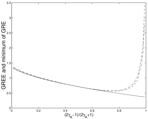
Figure 1: For type (i) gaussian state with $sinh(2r)=sinh(2r_{border})+5,x=1.1$, $(2\gamma_{B}-1)/(2\gamma_{B}+1)=0.5$. Solid line is for the searching result of type(i) border states which achieve GREE, dash for type(ii) state reaching the minimum of GRE within the type, dotted for type (iii),and dotted dash for type (iv).

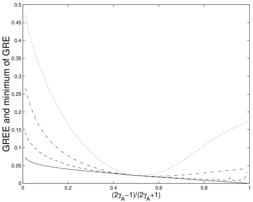
Figure 2: For type (ii) gaussian state with $sinh(2\theta)=0.5,x=x_{border}+1.5,(2\gamma_{B}-1)/(2\gamma_{B}+1)=0.5$. Solid line is for searching result of type(ii) border states which achieve GREE, dash for type(i) state reaching the minimum of GRE within the type, dotted for type (iii),and dotted dash for type (iv).

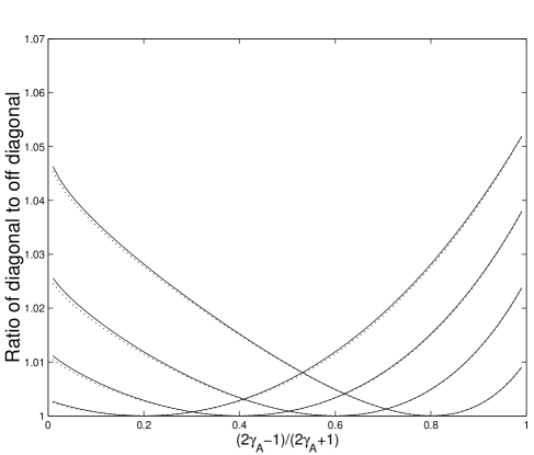
Figure 3: Solid lines are for original gaussian states whose $sinh(2r)=sinh(2r_{border})+5,x=1.1$, dotted for the border states which achieve GREE, In the left from up to down are for $(2\gamma_{B}-1)/(2\gamma_{B}+1)=0.2,0.4,0.6,0.8$ respectively

One the other hand, for symmetric Gaussian state (the type (iii) state), Based on the numerical observation, the conclusion can be drawn to be: for each type of state, GREE will be achieved by the same type of state.

For type (iii) state $\rho_{S}$ (symmetric gaussian state) characterized by CM of Eq. (12) and further by $m,k_{q},k_{p}$, the conclusion that GREE is achieved by symmetric Gaussian state can be strictly proven.Here I will give the main idea of proving. The detail will appear elsewhere. Let us start with the 6 parameters $M_{\sigma}$ as was done at the beginning of this section. This $6$ parameter EM can be produced as well as reduced to $\widetilde{M}_{\sigma}=diag\{\widetilde{M}_{A},\widetilde{M}_{B},$ $\widetilde{M}_{A},\widetilde{M}_{B}\}$ by symplectic transformation $S,$ $S^{T}M_{\sigma}S=\widetilde{M}_{\sigma},$ Now the $S$ matrix has $4$ parameters which are independent of the symplectic eigenvalues. The $S$ matrix takes the form of $S=S_{q}\oplus(S_{q}^{T})^{-1}$  It is known that symplectic transformation can always be dissolved to a rotation and squeezing then a successive rotation, that is $S=R_{2}DR_{1}$. with $R_{1}$ and $R_{2}$ are rotations and $D=diag\{d_{A},d_{B},1/d_{A},1/d_{B}\}$ is the squeezing operation. Now for the $q-p$ decorrelation form of $S,$ $S=S_{q}\oplus(S_{q}^{T})^{-1},$ $R_{1}$ and $R_{2}$ will be in their simple form of $R_{1}=\Theta\left(\theta\right)\oplus\Theta\left(\theta\right),$ and $R_{2}=\Theta\left(\phi\right)\oplus\Theta\left(\phi\right),$ By minimizing the relative entropy with respect to $\theta$ and $\phi$ under the restriction of $\sigma$ being a border state, one gets

$$\frac{\partial}{\partial\theta}\left(\frac{1}{2}Tr\alpha_{\rho}M_{\sigma}+\lambda c_{1}c_{2}\right)=\frac{\partial}{\partial\phi}\left(\frac{1}{2}Tr\alpha_{\rho}M_{\sigma}+\lambda c_{1}c_{2}\right)=0,$$ (40)

Where $\lambda$ is the multiplier. In general, the solution is quite complicate and involved with the other four parameters $d_{A},d_{B},\widetilde{M}_{A},\widetilde{M}_{B}$. But for the symmetric Gaussian state $\rho_{S}$, the solutions are quite simple. They are (i) $\sin\theta=0,$ $\tan\phi=\pm 1;$(ii) $\cos\theta=0,$ $\tan\phi=\pm 1.$ And the other four parameters $d_{A},d_{B},\widetilde{M}_{A},\widetilde{M}_{B}$ are not involved. The state $\sigma$ then will be the symmetric Gaussian state.

The GREE will be

$$E_{GR}\left(\rho_{S}\right) = Tr\rho_{S}\log\rho_{S}+\min_{\widetilde{M}_{A},\widetilde{M}_{B}}\{-\sum_{j=A,B}\log(2\sinh\frac{\widetilde{M}_{j}}{2})$$

$$+\frac{1}{2}[(m+k_{q})(m-k_{p})\widetilde{M}_{A}^{2}+(m-k_{q})(m+k_{p})\widetilde{M}_{B}^{2}$$

$$+(m-k_{q})(m-k_{p})\widetilde{M}_{A}\widetilde{M}_{B}\coth\frac{\widetilde{M}_{A}}{2}\coth\frac{\widetilde{M}_{B}}{2}$$

$$+(m+k_{q})(m+k_{p})\widetilde{M}_{A}\widetilde{M}_{B}\tanh\frac{\widetilde{M}_{A}}{2}\tanh\frac{\widetilde{M}_{B}}{2}]^{\frac{1}{2}},$$

where $\widetilde{M}_{j}=\log\frac{2\gamma_{j}+1}{2\gamma_{j}-1},$ and $\gamma_{j}$ are symplectic eigenvalues of border state. Here it is easy to prove that no further $X(x)$ operation is needed when the border state is prepared in its EM with the form of Eq. (14) (but with different parameters), that is to say $x=1$.

If $k_{p}=k_{q}$, the state will be two mode squeezed thermal state[15] $\rho_{ST}$. Then Eq. (5) is symmetric for $\widetilde{M}_{A},$ $\widetilde{M}_{B}$. Clearly the minimum will be achieved at $\widetilde{M}_{A}=$ $\widetilde{M}_{B}.$ So that

$$E_{GR}\left(\rho_{ST}\right) = Tr\rho_{ST}\log\rho_{ST}+\min_{\widetilde{M}_{A}}\{-2\log(2\sinh\frac{\widetilde{M}_{A}}{2})$$

$$+\frac{1}{2}\widetilde{M}_{A}[(m-k_{q})\coth\frac{\widetilde{M}_{A}}{2}+(m+k_{q})\tanh\frac{\widetilde{M}_{A}}{2}].$$

6 Conclusions and Discussions

Gaussian relative entropy of entanglement is an entanglement measure in its own right. The relative entropy between two gaussian states was expressed as correlation matrix of the first state and matrix in the exponential density operator of the second state. The mutual transform of $q-p$ fashion CM and EM was derived with symplectic transformation for $q-p$ decorrelation state. A most general transform of CM to EM and vice versa was given through commutation relation of the matrices and relation between the symplectic eigenvalues of the matrices. I proved that gaussian relative entropy of entanglement achieves when the separable gaussian state is at the border of separable and inseparable sets. The displacement or first moments of the second state can be ruled out as far as GREE is concerned. For GREE of $1\times 1$ gaussian state, the ten parameters EM of separable state which minimizes the relative entropy was reduced to three variables EM. Where the matrix was decomposed as local operations applied to a standard form of EM. The three variables in EM were left for numerical calculation of the minimization. To construct an EM more suitable for the calculation of GREE, I classified the standard form CM of $1\times 1$ gaussian state into four types according to some kind of ratio of diagonal to off diagonal for the first three types and symmetry for the fourth. The numeric evidence on the minimization of EMs strongly suggests that GREE for each type of gaussian state will be realized by the state within the same type.

I strictly proved that GREE for symmetric Gaussian state is achieved by symmetric gaussian state.It was given as the minimization of a function on the two symplectic eigenvalues of EM. Although the minimization equations are easily obtained, but they can not be solved analytically. Further more, for a special kind of the symmetric state, the two mode squeezed thermal state (TMST), the GREE will be a minimization of a function on one parameter, the symplectic eigenvalue of TMST, and the state achieves the GREE is a TMST state. I and my coworker had calculated [15]the minimization of relative entropy of TMST with respect to TMST as the upper bound of relative entropy of entanglement, now it is proved that it is just the GREE of TMST. Moreover, the upper bound for entanglement of formation proposed in the same paper turns out to be the entanglement of formation itself [16]. So the comparison of the upper bound of EoF and RE of TMST in our former paper [15] is in fact the comparison of EoF and GREE. And we had also provided coherent information and other entanglement measure such as logarithmic negativity in that comparison.

I have given the method to calculate GREE for general state and the detail calculation of GREE for $1\times 1$ gaussian state. It is expected that the method developed in this paper will be applicable to the multi-mode bipartite gaussian states and multipartite gaussian states.The definition of  GREE need not limit to gaussian state. For a non gaussian continuous variable state, GREE can also be defined as the minimization of relative entropy of the state with respect to all separable gaussian state. But there is a deficiency that the relative entropy will never be zero. Never the less, the calculation involves only the first and second moments of the state, the necessary condition of separability on the CM of the non gaussian state was also addressed [7], and the logarithmic of separable gaussian state can be treated with EM.

Acknowledgment: Funding by the National Natural Science Foundation of China (under Grant No. 10347119) is gratefully acknowledged.

References

• [1] B. W. Schumacher and M. D. Westmoreland, lanl eprint no. quant-ph/0004045. (2000),
• [2] V.Vedral , M. B. Plenio, M. A. Rippin, and P. L. Knight, , Phys. Rev. Lett. 78, 2275 (1997).V. Vedral, Rev. Mod. phys. 74, 197 (2002). V.Vedral., M. B. Plenio, K. Jacobs, and P. L. Knight,, Phys. Rev. A 56, 4452 (1997).
• [3] Sheng-Jun Wu, et al,Chinese Phys. Lett. 18 160 (2001); quant-ph/0004018.
• [4] Β J. Eisert, C. Simon, M.B.Plenio, J. Phys. A 35 3911 (2002).
• [5] S. Scheel and D-G Welsch , Phys. Rev. A 64 063811 (2001).
• [6] L. M. Duan, G. Giedke, J. I. Cirac and P. Zoller, Phys. Rev. Lett. 84, 2722 (2000).
• [7] R. Simon, Phys. Rev. Lett. 84, 2726 (2000),
• [8] G. Giedke, B. Kraus, M. Lewenstein, and J. I. Cirac,Β Β Phys. Rev. Lett. 87 167904 (2001).
• [9] Xiang-Bin Wang, M. Keiji, T. Akihisa,Β Β Phys. Rev. Lett. 87 137903 (2001).
• [10] Xiang-Bin Wang, et al Β J. Phys. A. 27 6563 (1994).
• [11] A. S. Holevo, M. Sohma, and O. Hirota, Phys. Rev. A 59, 1820 (1999).
• [12] E. Leib and M. B. Ruskai, Phys. Rev. Lett. 30, 434 (1973); E. Leib and M. B. Ruskai, J. Math. Phys. 14, 1938 (1973).
• [13] A. Holevo and R. F. Werner, Phys. Rev. A 63, 032312 (2001), quant-ph/9912067.
• [14] G. Vidal and R. F. Werner, Phys. Rev. A 65, 032314 (2002), quant-ph/0102117.
• [15] Xiao-yu Chen, Pei-liang Qiu, Phys. Lett. A, 314, 191(2003).
• [16] G. Giedke, M. M. Wolf, O. Kruger, R. F. Werner, and J. I. Cirac ,Phys. Rev. Lett.Β 91, 107901 (2003).