Simulating noisy quantum protocols with quantum trajectories

Abstract

The theory of quantum trajectories is applied to simulate the effects of quantum noise sources induced by the environment on quantum information protocols. We study two models that generalize single qubit noise channels like amplitude damping and phase flip to the many-qubit situation. We calculate the fidelity of quantum information transmission through a chaotic channel using the teleportation scheme with different environments. In this example, we analyze the role played by the kind of collective noise suffered by the quantum processor during its operation. We also investigate the stability of a quantum algorithm simulating the quantum dynamics of a paradigmatic model of chaos, the baker’s map. Our results demonstrate that, using the quantum trajectories approach, we are able to simulate quantum protocols in the presence of noise and with large system sizes of more than 20 qubits.

I Introduction

It would be highly desirable to implement quantum protocols using processors perfectly isolated from the environment, since this is one of the main sources of error in quantum computation (there are also system specific imperfections, but here we will only address the environmental problem). Unfortunately, this is not possible. Quantum hardware will naturally become entangled with the environment during its operation. Thus, if any hope of profiting from the benefits of quantum computation is to be kept, understanding and controlling quantum noise effects is essential. On the other hand, the study of open systems is of interest in several fields, from both theoretical and experimental points of view Gra1 ; Gra2 ; Gra3 ; Knight .

Factoring large integers in polynomial time has been the milestone discovery that set out quantum computation as a major research topic shor . Nevertheless, in the short term, few qubits quantum computers, this kind of calculations will be necessarily out of reach, since they involve large systems. Then, it is reasonable to focus on understanding the behavior of accessible first realizations. It is interesting to remark that, with a few tens of qubits, quantum simulations of systems studied in quantum chaos (like the quantum baker’s map Sch , the quantum kicked rotator Bertrand , and the quantum sawtooth map Ben1 ) would outperform any calculation that can be done with present day supercomputers. A first step in the simulation of quantum chaos models has been the implementation of the quantum baker’s map on a three-qubit NMR-based quantum processor cory .

With this situation in mind, it is natural to ask to what extent we can know and control the operability and the stability of a quantum computer of this size. Theoretical studies rely on evaluating the reduced density matrix of the system (obtained after tracing out the environment), often in terms of various different approximations. It would therefore be desirable to give an answer for generic quantum protocols and noise models, using exact calculations. In this work, we propose the numerical simulation of superoperators as a way to do it. By means of quantum trajectories techniques we can reach results for system sizes for which the implementation of chaotic maps becomes relevant for theoretical studies in the field of quantum chaos, having the chance to include any kind of environmental effects.

Instead of solving the density matrix directly, quantum trajectories stochastically evolve the state vector of the system, and after averaging over many runs the same results for the outcomes of any observable are obtained. The use of quantum trajectories in the field of quantum information has been pioneered by Schack ; BarencoBrun . In Ref. Car , we applied this formalism to study the effect of a dissipative environment on the quantum teleportation protocol BennettBrassard through a large chain of qubits. This situation models the transmission of quantum information through a chaotic quantum channel. Here we review this model and present new results for different noise channels.

As mentioned before, one of the main near future applications of quantum computation is the simulation of dynamical systems that are of great interest in quantum chaos. In this work we focus on the quantum baker’s map, one of the most important examples of this kind of systems. This map is fully chaotic and its quantized version consists of conveniently selected quantum Fourier transforms. We model the environment through a phase flip channel and study the fidelity of quantum computing of the quantum baker’s map in this noisy environment. We note that the fidelity has already been computed experimentally with a three-qubit NMR quantum processor cory . Hence, for the design and construction of quantum hardware with a larger number of qubits, simulations like those performed in this paper will become essential.

This paper is organized as follows. In Sec. II, we present a brief explanation of the theory of quantum trajectories and connect it with the quantum operations approach to the density matrix evolution. We also refer to the master equation formulation. Afterward, in Sec. III, we make a short description of the noise channels that we use in the calculations, paying special attention to the amplitude damping models. In Sec. IV, we review the quantum teleportation protocol presented in Car , focusing on the different dissipative processes. In Sec. V, we study the behavior of the fidelity of the quantum algorithm for the baker’s map in the presence of a phase flip noise. Finally, in Sec. VI, we present our conclusions and outlook.

II Master equation, superoperators, and quantum trajectories

There is a close relationship among the master equation in Lindblad form, the superoperator formalism and the quantum trajectories theory. It is useful to review this relationship and to motivate the use of the quantum trajectory approach when studying open systems like quantum processors. We start with the special case of the master equation formulation of the problem and relate it with simulations using quantum trajectories techniques. Then, in Sec. II.2 we generalize this establishing the connection with the broader quantum operators formalism.

II.1 Master equation and quantum trajectories

Real systems interact with the environment, and, as mentioned before, these interactions are usually referred to as quantum noise Chuangbook ; Preskillbook . Several models account for different sorts of system-environment interactions, the particular choice depending on the nature of the system and environment under consideration. Such open quantum systems in general cannot be described by a pure state, but rather by a mixed state. Their evolution takes density matrices to density matrices. This allows the evolution from system’s pure states to mixed ones, and also, in some noise models, from mixed to pure states. In order to obtain the differential equation corresponding to this process, one assumes Markovian behavior, giving the evolution of the density operator with reference only to its state at present. This Markovian assumption neglects memory effects: it implies that the time needed for the environment to loose the information it received from the system is short enough in comparison with the time scale of the dynamics we perceive. Then, we are entitled to regard the information flow in only one direction, neglecting any kind of feedback Preskillbook .

The Lindblad form of the master equation of this system-environment model in the Born-Markov approximation can be formally written as Lindblad :

$$\dot{\rho}={\cal L}[\rho],$$ (1)

with formal solution

$$\rho(t)=\exp({\cal L}t)[\rho(0)],$$ (2)

where ${\cal L}$ stands for the “Lindblandian” operator. In order to obtain explicit expressions we can trace out the environment, which gives

$$\dot{\rho}=-\frac{i}{\hbar}[H_{s},\rho]-\frac{1}{2}\sum_{\mu}\{L_{\mu}^{{\dagger}}L_{\mu},\rho\}+\sum_{\mu}L_{\mu}\rho L_{\mu}^{{\dagger}},$$ (3)

where $L_{\mu}$ are the Lindblad operators ($\mu\;\epsilon\;[1,\ldots,{\cal M}]$, the number ${\cal M}$ depending on the noise model), $H_{s}$ is the system’s Hamiltonian and { , } denotes the anticommutator. The first two terms of this equation can be regarded as the evolution performed by an effective non-Hermitian Hamiltonian, $H_{\rm eff}=H_{s}+iK$, with $K=-\hbar/2\sum_{\mu}L_{\mu}^{{\dagger}}L_{\mu}$. In fact, we see that

$$-\frac{i}{\hbar}[H_{s},\rho]-\frac{1}{2}\sum_{\mu}\{L_{\mu}^{{\dagger}}L_{\mu},\rho\}=-\frac{i}{\hbar}[H_{\rm eff}\rho-\rho H_{\rm eff}^{\dagger}],$$ (4)

which reduces to the usual evolution equation for the density matrix in the case of $H_{\rm eff}$ being Hermitian. The last term is responsible for the so-called quantum jumps. In this context the Lindblad operators $L_{\mu}$ are also named quantum jump operators. If the initial density matrix is in a pure state $\rho(t_{0})=|\phi(t_{0})\rangle\langle\phi(t_{0})|$, after a time $dt$ evolves to the following statistical mixture:

$$\rho(t_{0}+dt)=(1-\sum_{\mu}dp_{\mu})\>|\phi_{0}\rangle\langle\phi_{0}|\>+\sum_{\mu}dp_{\mu}|\phi_{\mu}\rangle\langle\phi_{\mu}|,$$ (5)

with the probabilities $dp_{\mu}$ defined by

$$dp_{\mu}\!=\!\langle\phi(t_{0})|L_{\mu}^{{\dagger}}L_{\mu}|\phi(t_{0})\rangle dt,$$ (6)

and the new states by

$$|\phi_{0}\rangle=\frac{(\openone-iH_{\rm eff}dt/\hbar)|\phi(t_{0})\rangle}{\sqrt{1-\sum_{\mu}dp_{\mu}}}$$ (7)

and

$$|\phi_{\mu}\rangle=\frac{L_{\mu}|\phi(t_{0})\rangle}{||L_{\mu}|\phi(t_{0})\rangle||}.$$ (8)

Then, the quantum jump picture turns out to be clear; with probability $dp_{\mu}$ a jump occurs and the system is prepared in the state $|\phi_{\mu}\rangle$. With probability $1-\sum_{\mu}dp_{\mu}$ there are no jumps and the system evolves according to the effective Hamiltonian $H_{\rm eff}$ (normalization is included also in this case because the evolution is given by a non-unitary operator).

The numerical method we are going to use in order to simulate the master equation is usually known as the Monte Carlo Wave function approach DalibardCastin . We start from a pure state $|\phi(t_{0})\rangle$ and at intervals $dt$, smaller than the timescales relevant for the evolution of the density matrix, we perform the following evaluation. We choose a random number $\epsilon$ from a uniform distribution in the unit interval $[0,1]$. If $\epsilon<dp$, where $dp=\sum_{\mu}dp_{\mu}$, the system jumps to one of the states $|\phi_{\mu}\rangle$ (to $|\phi_{1}\rangle$ if $0\leq\epsilon\leq dp_{1}$, to $|\phi_{2}\rangle$ if $dp_{1}<\epsilon\leq dp_{1}+dp_{2}$, and so on). On the other hand, if $\epsilon>dp$, the evolution with the non-Hermitian Hamiltonian $H_{\rm eff}$ takes place, ending up in the state $|\phi_{0}\rangle$. In both circumstances we renormalize the state. We repeat this process as many times as $n_{\rm steps}=\Delta t/dt$ where $\Delta t$ is the whole elapsed time during the evolution. Note that we must take $dt$ much smaller than the time scales relevant for the evolution of the open quantum system under investigation. In our simulations, $n_{\rm steps}$ will be proportional to the number of quantum gates involved in the corresponding protocol. Each realization provides a different quantum trajectory and a particular set of them (given a choice of the Lindblad operators) is an “unraveling” of the master equation. It is easy to see that if we average over different runs we recover the probabilities obtained with the density operator. In fact, given an operator $A$, we can write the mean value $\langle A\rangle_{t}={\rm Tr}[A\rho(t)]$ as the average over ${\cal N}$ trajectories:

$$\langle A\rangle_{t}=\lim_{{\cal N}\to\infty}\frac{1}{{\cal N}}\sum_{i=1}^{{\cal N}}\langle\phi_{i}(t)|A|\phi_{i}(t)\rangle.$$ (9)

The advantage of using the quantum trajectories method is clear since we need to store a vector of length $N$ ($N=2^{n}$ is the dimension of the Hilbert space, $n$ being the number of qubits) rather than a $N\times N$ density matrix. Moreover, there is also an advantage in computation time with respect to density matrix direct calculations. We find that a reasonable amount of trajectories (we have used $100\leq{\cal N}\leq 400$ in all calculations, unless otherwise mentioned) is needed in order to obtain a satisfactory statistical convergence.

This picture can be formalized by means of the stochastic Schrödinger equation Brun

$$|d\phi\rangle = -iH_{s}|\phi\rangle dt-\frac{1}{2}\sum_{\mu}(L_{\mu}^{{\dagger}}L_{\mu}-\langle L_{\mu}^{{\dagger}}L_{\mu}\rangle_{\phi})|\phi\rangle\>dt$$ (10)

$$+\sum_{\mu}\left(\frac{L_{\mu}}{\sqrt{\langle L_{\mu}^{{\dagger}}L_{\mu}\rangle_{\phi}}}-\openone\right)|\phi\rangle\>dN_{\mu}.$$

This is a stochastic nonlinear differential equation, where the stochasticity is due to the measurement results: we think that the environment is actually measured (as it is the case in indirect measurement models) or simpler, that the contact of the system with the environment produces an effect similar to a continuous measurement Zurek . The nonlinearity is due to the renormalization of the state vector. The stochastic differential variables $dN_{\mu}$ are statistically independent and represent measurement outcomes. Their ensemble mean is given by $M[dN_{\mu}]=\langle L_{\mu}^{{\dagger}}L_{\mu}\rangle_{\phi}dt$. The probability that the variable $dN_{\mu}$ is equal to $1$ during a given time step $dt$ is $\langle\phi L_{\mu}^{\dagger}L_{\mu}\phi\rangle\>dt$. Therefore, most of the time the variables $dN_{\mu}$ are $0$ and as a consequence the system evolves continuously by means of the non Hermitian effective Hamiltonian. However, when a variable $dN_{\mu}$ is equal to $1$, the corresponding term in equation (10) is the most significant. In these cases the quantum jump occurs. Note that there are also other possibilities in order to unravel the master equation such as the quantum state diffusion GisinPercival ; Schack , for example.

II.2 Quantum operations and quantum trajectories

There is a close connection between the master equation in Lindblad form and the quantum operations theory Chuangbook ; Preskillbook and we use this latter formalism as a comparison tool for the quantum trajectories calculations. Furthermore, it will become clear that the evolution of the density matrix of the system given by this method can be put on the same footing as the stochastic evolution model. In fact, the latter constitutes a Monte Carlo simulation of the former.

We write the solution to Eq. (3) over an infinitesimal time $dt$ as a completely positive map:

$$\rho(t+dt)=\$[\rho(t)]=\sum_{\mu=0}^{{\cal M}}M_{\mu}(dt)\rho(t)M_{\mu}^{{\dagger}}(dt),$$ (11)

where, for $\mu=0$, we have $M_{0}=\openone-iH_{\rm eff}dt/\hbar$ and, for $\mu>0$, $M_{\mu}=L_{\mu}\sqrt{dt}$, satisfying $\sum_{\mu=0}^{\cal M}M_{\mu}^{{\dagger}}M_{\mu}=\openone$ to first order in $dt$. Equation (11) is called the Kraus representation (or the operator sum representation) of the superoperator $\$$ and the operators $M_{\mu}$ are known as operators elements for the quantum operation $\$$. It can be shown that, if the global evolution (system plus environment) is unitary, the Kraus operators satisfy the completeness relation $\sum_{\mu=0}^{\cal M}M_{\mu}M_{\mu}^{{\dagger}}=\openone$ Chuangbook ; Preskillbook . Note that the superoperator $\$$ maps density matrices to density matrices, that is $\rho(t+dt)$ is Hermitian, has unit trace and is nonnegative if $\rho(t)$ satisfies these properties.

The action of the quantum operation $\$$ can be interpreted as $\rho$ being randomly replaced by $M_{\mu}\rho M_{\mu}^{{\dagger}}/{\rm Tr}(M_{\mu}\rho M_{\mu}^{{\dagger}})$, with probability ${\rm Tr}(M_{\mu}\rho M_{\mu}^{{\dagger}})$. Equivalently, the set $\{M_{\mu}\}_{\mu=1,...,{\cal M}}$ defines a Positive Operator Valued Measurement (POVM) with operators $E_{\mu}=M_{\mu}^{{\dagger}}M_{\mu}$, that satisfy $\sum_{\mu=0}^{\cal M}E_{\mu}=\openone$. The outlined process is equivalent to performing a continuous measurement on the system (or an indirect measurement if the environment is actually measured) and shows the close connection between the Kraus operators formalism and the quantum jumps picture.

We would like to mention that the quantum operations formalism is more general than the master equation approach. The operator sum formulation in differential form can be obtained from the master equation, but a general quantum process described in terms of an operator sum representation needs to be Markovian in order to be tractable with a master equation. This opens the possibility of studying a wide range of non Markovian phenomena using quantum trajectories simulations.

III Noise channels

There are several ways to model the interaction of a system with the environment. The most common examples found in the literature are the amplitude damping channel, the phase flip channel, and the depolarizing channel Chuangbook ; Preskillbook . In this section, we give a brief description of two relevant noise models (amplitude damping and phase damping) in the single qubit case, and then we generalize them to $n$-qubit systems.

Dissipation (energy loss) is one of the main features present in open quantum systems. Different phenomena like, for example, spontaneous atomic emission of a photon or spin systems approaching equilibrium can be modeled by this quantum operation, i.e., the amplitude damping. Considering the environment initially in the vacuum state $|0\rangle_{e}$, there is a probability $p$ that the excited state of the system decays and that the state of the environment changes from the vacuum to $|1\rangle_{e}$.

$$|0\rangle_{s}|0\rangle_{e} \rightarrow |0\rangle_{s}|0\rangle_{e},$$

$$|1\rangle_{s}|0\rangle_{e} \rightarrow \sqrt{1-p}\;|1\rangle_{s},|0\rangle_{e}+\sqrt{p}\;|0\rangle_{s}|1\rangle_{e},$$ (12)

where $|0\rangle_{s}$ stands for the spin down (ground) state and $|1\rangle_{s}$ for the spin up (excited) state of the system, and the indexes $s$ and $e$ denote the quantum states of the system and of the environment, respectively. Tracing out the environment the corresponding Kraus operators are obtained:

$$M_{0}=\left(\begin{array}[]{cc}1&0\\ 0&\sqrt{1-p}\\ \end{array}\right),\quad M_{1}=\left(\begin{array}[]{cc}0&\sqrt{p}\\ 0&0\\ \end{array}\right).$$ (13)

The operator $M_{1}$ is responsible for the quantum jumps and $M_{0}$ for the continuous evolution. For the case of infinitesimal evolution operators (see Sec. II), a repeated application of this noise channel gives an exponential decay law of the population of the state $|1\rangle$ Preskillbook . Therefore, this evolution drives any intial (pure or mixed) state of the qubit to the pure state $|0\rangle$. Note that here and in the following the matrix representations of the single-qubit Kraus operators are written in the $\{|0\rangle,|1\rangle\}$ basis.

We also consider the phase flip channel (which is equivalent to the phase damping channel Chuangbook ) given by the following model

$$|0\rangle_{s}|0\rangle_{e} \rightarrow \sqrt{1-p}\;|0\rangle_{s}|0\rangle_{e}+\sqrt{p}\;|0\rangle_{s}|1\rangle_{e},$$

$$|1\rangle_{s}|0\rangle_{e} \rightarrow \sqrt{1-p}\;|1\rangle_{s}|0\rangle_{e}-\sqrt{p}\;|1\rangle_{s}|1\rangle_{e},$$ (14)

with Kraus operators

$$M_{0}=\sqrt{1-p}\;\left(\begin{array}[]{cc}1&0\\ 0&1\\ \end{array}\right),\quad M_{1}=\sqrt{p}\;\left(\begin{array}[]{cc}1&0\\ 0&-1\\ \end{array}\right).$$ (15)

This kind of noise can be thought as describing quantum information loss, in contrast with the previous model, which describes energy loss. This is a purely quantum mechanical process and has been extensively studied in the context of quantum to classical correspondence Zurek .

In order to generalize the single qubit amplitude damping process to many qubits we will follow two different points of view. In the first case we assume that a single damping probability describes the action of the environment, irrespective of the internal many-body state of the system. In the second approach, we assume that each qubit has its own interaction with the environment, independently of the other qubits. This makes the damping probability grow with the number of qubits that can perform the transition $|1\rangle\to|0\rangle$. Both models assume that only one qubit of the system can decay at a time.

In the first case Car , we have a probability $p$ for the system to perform one of the possible transitions, each of them being equally likely. This can be illustrated with a two-qubit example:

$$|00\rangle_{s}|00\rangle_{e} \rightarrow |00\rangle_{s}|00\rangle_{e},$$

$$|01\rangle_{s}|00\rangle_{e} \rightarrow \sqrt{1-p}\>|01\rangle_{s}|00\rangle_{e}+\sqrt{p}\>|00\rangle_{s}|01\rangle_{e},$$

$$|10\rangle_{s}|00\rangle_{e} \rightarrow \sqrt{1-p}\>|10\rangle_{s}|00\rangle_{e}+\sqrt{p}\>|00\rangle_{s}|10\rangle_{e},$$

$$|11\rangle_{s}|00\rangle_{e} \rightarrow \sqrt{1-p}\>|11\rangle_{s}|00\rangle_{e}+\sqrt{p/2}$$ (16)

$$(|10\rangle_{s}|01\rangle_{e}+|01\rangle_{s}|10\rangle_{e}).$$

A $n$-qubit state $|i_{n-1}\ldots i_{0}\rangle$ ($i_{l}=0,1$, with $0\leq j\leq n-1$) decays in the interval $dt$ with a probability $p=\Gamma dt/\hbar$. After this infinitesimal time, the possible states of the system are those in which the damping $|1\rangle\to|0\rangle$ has occurred in one of the qubits, the damping probability being the same for all the qubits. We provide a compact expression for the Kraus operators $M_{\mu}$ in our model, following the formulation given in Sec. II.2 for the infinitesimal evolution. The matrix elements for the $k$th operator in the computational basis $|i\rangle\equiv|i_{n-1}\ldots i_{0}\rangle$, with $i\equiv\sum_{l=0}^{n-1}i_{l}2^{l}$, are given by

$$[M_{\mu}^{(n)}]_{i,j}=\left\{\begin{array}[]{ll}\sqrt{\frac{\Gamma dt}{\hbar\sum_{l=0}^{n-1}i_{l}}},&\;{\rm for}\;j\geq 2^{(\mu-1)},\\ &i=j-2^{(\mu-1)},\\ &i_{l}=0,1,\\ &\\ 0&\;{\rm otherwise},\end{array}\right.$$ (17)

where the superscript ⁽ⁿ⁾ in $M_{\mu}^{(n)}$ underlines the fact that we are dealing with $n$-qubit Kraus operators. There are $n$ operators $M_{\mu}^{(n)}$ ($\mu=1,\ldots,n$), where the index $\mu$ singles out which qubit undergoes the transition $|1\rangle\to|0\rangle$. The $M_{0}^{(n)}$ operator is

$$[M_{0}^{(n)}]_{i,j}=\left\{\begin{array}[]{ll}1&\;{\rm for}\;i=j=0,\\ \sqrt{1-\frac{\Gamma dt}{\hbar}}&\;{\rm for}\;i=j\neq 0,\\ &\\ 0&\;{\rm otherwise}.\end{array}\right.$$ (18)

Note that, if we replace in the above definition the square root by its first order approximation, we arrive at the same expression for the action of the effective Hamiltonian given in Sec. II (see the first term in the right hand side of Eq. (5) and Eq. (7)).

For example, starting from the four-qubit pure state $\rho(t_{0})=|1011\rangle\langle 1011|$, the action of the generalized amplitude damping channel leads, after a time $dt$, to the statistical mixture

$$\rho(t_{0}+dt)=\left(1-\frac{\Gamma dt}{\hbar}\right)|1011\rangle\langle 1011|+\frac{\Gamma dt}{3\hbar}(|0011\rangle\langle 0011|$$

$$+|1001\rangle\langle 1001|+|1010\rangle\langle 1010|).$$ (19)

This situation can be described as branching process or a cascade in the population of different classes of states (see, e.g., Ref. Flam ). A class in this model is naturally defined as the collection of all the states of the system having the same number of qubits in the “up” state (i.e., of $|1\rangle$ states). The first class is the one initially populated with probability $W_{0}$. The second class, with associated probability $W_{1}$, corresponds to the states that are obtained from the initial state after the damping of one qubit. The third class, with probability $W_{2}$, includes the states that can be reached by the damping of one qubit in any of the states of the second class, and so on until reaching the “ground state” $|0\ldots 0\rangle$ of the system. This last state is also the only state that resides in the last class. This class is populated with probability $W_{m}$, the number $m$ being the maximum number of up spins in the initial state (if we start from a state $|i_{n-1}\ldots i_{0}\rangle$ of the computational basis, then $m=\sum_{l=0}^{n-1}i_{l}$). Note that $m\leq n$. The set of probabilities $W_{m}$ can be obtained by means of the following differential equations:

$$\frac{dW_{0}}{dt} = -\frac{\Gamma}{\hbar}\;W_{0},$$

$$\vdots$$

$$\frac{dW_{k}}{dt} = \frac{\Gamma}{\hbar}\;(W_{k-1}-W_{k}),$$

$$\vdots$$

$$\frac{dW_{m}}{dt} = \frac{\Gamma}{\hbar}\;W_{m-1},$$ (20)

with solutions

$$W_{k} = \frac{(\Gamma t/\hbar)^{k}}{k!}\;\exp{\left(-\frac{\Gamma t}{\hbar}\right)},$$

$$W_{m} = 1-\sum_{k=0}^{m-1}W_{k}.$$ (21)

In Fig. 1 we show a comparison among the probabilities for each class obtained with quantum trajectories simulations and the theoretical formulae, in the case of $n=6$. We have evolved the initial state $|2^{n}-1\rangle=|1\ldots 1\rangle$ up to time $2n\;dt$, for different values of the dimensionless damping rate $\gamma=\Gamma dt/\hbar$. This evolution is purely dissipative, without considering any other kind of system’s dynamics. As can be seen from Fig. 1, we have a very good agreement between quantum trajectories numerical simulations and the theoretical predictions of the model.

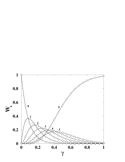
Figure 1: Probabilities $W_{k}$ for each class of states in terms of the dimensionless damping rate $\gamma=\Gamma dt/\hbar$, in a system with $n=6$ qubits, obtained after evolving the initial state $|1\ldots 1\rangle$ up to time $2ndt$, under the noise model (17). Solid lines correspond to the exact formulae (21), and the numbers close to each curve indicate the corresponding class. Diamonds stand for quantum trajectories simulations (error bars are not shown since they are smaller than the size of the symbols).

The other generalization for the amplitude damping differs from the previous one in that the decay probability is now the same for each single qubit process, independently of the state of the system. Then, the decay probability for a states of the computational basis is proportional to the number of qubits in the up state. This can be illustrated in the two-qubit case. In this example, the noise channel is described by the following unitary evolution formulae:

$$|00\rangle_{s}|00\rangle_{e} \rightarrow |00\rangle_{s}|00\rangle_{e},$$

$$|01\rangle_{s}|00\rangle_{e} \rightarrow \sqrt{1-p}\>|01\rangle_{s}|00\rangle_{e}+\sqrt{p}\>|00\rangle_{s}|01\rangle_{e},$$

$$|10\rangle_{s}|00\rangle_{e} \rightarrow \sqrt{1-p}\>|10\rangle_{s}|00\rangle_{e}+\sqrt{p}\>|00\rangle_{s}|10\rangle_{e},$$

$$|11\rangle_{s}|00\rangle_{e} \rightarrow \sqrt{1-2p}\>|11\rangle_{s}|00\rangle_{e}+\sqrt{p}$$ (22)

$$(|10\rangle_{s}|01\rangle_{e}+|01\rangle_{s}|10\rangle_{e}).$$

The Kraus operators $M_{\mu}^{(n)}$ for this model are given by the $n$-factor tensor product

$$M_{\mu}^{(n)}=\openone\otimes\ldots\otimes M_{1}\otimes\ldots\otimes\openone,$$ (23)

where $M_{1}$ is given by Eq. (13) and $\mu$ ($\mu=1,\ldots,n$) coincides with the position of $M_{1}$ in (23), that is $\mu$ singles out the qubit which decays from $|1\rangle$ to $|0\rangle$. In the computational basis, the matrix representation of the operator $M_{0}^{(n)}$ is given by

$$[M_{0}^{(n)}]_{i,j}=\left\{\begin{array}[]{ll}1&\;{\rm for}\;i=j=0,\\ \sqrt{1-\sum_{l=0}^{n-1}i_{l}\frac{\Gamma dt}{\hbar}}&\;{\rm for}\;i=j\neq 0,\\ &\\ 0&\;{\rm otherwise}.\end{array}\right.$$ (24)

The evolution of the pure state $\rho(t_{0})=|1011\rangle\langle 1011|$ is different from what obtained in the previous many-qubit damping model (see Eq. (19). We have

$$\rho(t_{0}+dt)=\left(1-\frac{3\Gamma dt}{\hbar}\right)|1011\rangle\langle 1011|+\frac{\Gamma dt}{\hbar}(|0011\rangle\langle 0011|$$

$$+|1001\rangle\langle 1001|+|1010\rangle\langle 1010|).$$ (25)

The cascade in the population of the different classes $W_{k}$ is ruled by the following set of differential equations:

$$\frac{dW_{0}}{dt} = -\frac{\Gamma}{\hbar}\;n_{0}\;W_{0},$$

$$\vdots$$

$$\frac{dW_{k}}{dt} = \frac{\Gamma}{\hbar}\;(n_{k-1}\;W_{k-1}-n_{k}\;W_{k}),$$

$$\vdots$$

$$\frac{dW_{m}}{dt} = \frac{\Gamma}{\hbar}\;n_{m-1}\;W_{m-1}=\frac{\Gamma}{\hbar}{W_{m-1}},$$ (26)

where $n_{k}$ is the number of qubits in the “up” state for the class $k$. Taking into account that $n_{k}=n_{0}-k=m-k$, the solutions are

$$W_{k} = \frac{n!}{n_{k}!}\;\sum_{i=0}^{k}\frac{(-1)^{(k-i)}}{i!\>(k-i)!}\;\exp{\left(-\frac{n_{i}\>\Gamma t}{\hbar}\right)},$$

$$W_{m} = 1-\sum_{k=0}^{m-1}W_{k}.$$ (27)

In Fig. 2, we take the initial state $|2^{n}-1\rangle$ evolving it for a time $n\;dt$, for different values of the dimensionless damping rate $\gamma$. Again, only dissipation is considered and we have found a very good agreement with our analytical predictions.

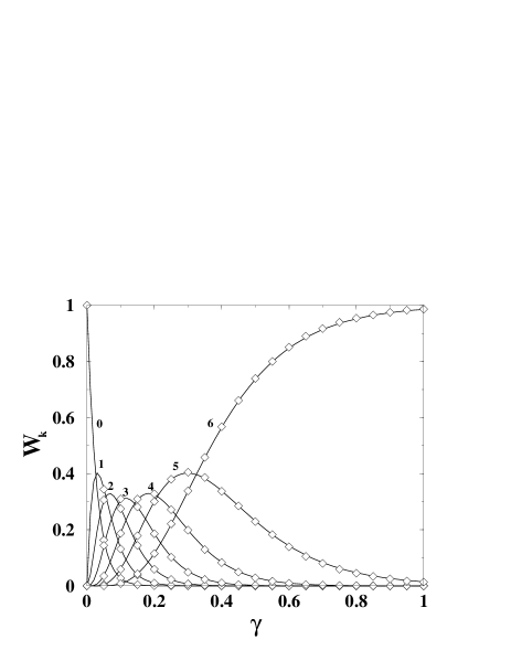
Figure 2: Same as in Fig. 1, but for the noise model (23) and after evolution up to time $ndt$.

With this same idea we generalize the phase flip channel. The Kraus operators are given by the $n$-factor tensor product of Eq. (23), where now $\mu$ ($\mu=1,\ldots,n$) coincides with the position of the matrix $M_{1}$ of Eq. (15), instead of Eq. (13). The matrix representation of the Kraus operator $M_{0}^{(n)}$ in the computational basis is

$$[M_{0}^{(n)}]_{i,j}=\left\{\begin{array}[]{ll}\sqrt{1-n\frac{\Gamma dt}{\hbar}}&\;{\rm for}\;i=j,\\ &\\ 0&\;{\rm otherwise}.\end{array}\right.$$ (28)

We study the stability of a given state vector subjected to this decoherence channel. Namely, we compute the fidelity $F={\rm Tr}[\rho_{0}\rho(t)]$ of a $n$-qubit system, for a random initial state $|\psi_{0}\rangle$, as a function of $\gamma=\Gamma dt/\hbar$ ($\rho_{0}=|\psi_{0}\rangle\langle\psi_{0}|$ is the density matrix for the initial state and $\rho(t)$ is the density matrix of the system at time $t$). All components of the initial random state vector $|\psi_{0}\rangle$ are taken to be random complex numbers of modulus $1/\sqrt{2^{n}}$. A combinatorial calculation provides an exact closed expression for the fidelity in this case. We obtain

$$F(t)=\frac{1}{2^{n}}+\frac{n!}{2^{n}}\>\sum_{i=1}^{n}\frac{1}{i!\>(n-i)!}\>\exp{\left(-\frac{2i\>\Gamma t}{\hbar}\right)}.$$ (29)

Note that this formula does not give a simple exponential fidelity decay, but a superposition of exponential decays with different rates, since the decay rate depends on the number of up spins in the different states of the computational basis.

The agreement of the quantum trajectories simulations with this theoretical formula is shown in Fig. 3. The semi log version of the theoretical curve is shown in the inset, where we plot $F-F_{\infty}$, $F_{\infty}=1/2^{n}$ being the asymptotic value of fidelity at $t=\infty$ or at $\Gamma=\infty$. We note that the asymptotic decay of $\bar{F}=F-F_{\infty}$ takes place with the lowest decay rate $\Gamma_{1}=2\Gamma/\hbar$. of Eq. (29).

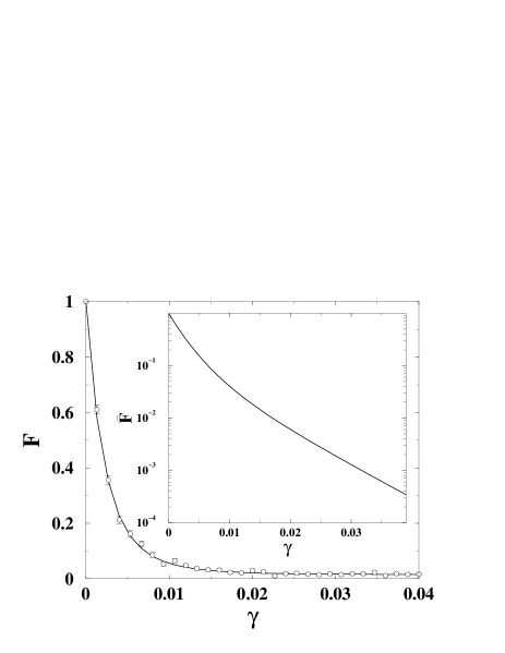
Figure 3: Fidelity of a random initial state in terms of the dimensionless decay rate $\gamma=\Gamma dt/\hbar$, in a system with $n=6$ qubits, subjected to the generalized phase flip channel up to time $2n^{2}dt$. The very good agreement between quantum trajectories simulations (circles with error bars) and theoretical predictions (solid line) is clearly seen. Here and in the following figures the error bars give the size of the statistical error. The inset shows the semi log version of the theoretical curve plot for the modified fidelity $\bar{F}=F-F_{\infty}$.

We note that analytical formulae for fidelity decay can also be found for other special initial conditions. For instance, Eq. (29) remains valid when the initial state is a random superposition of computational basis states with up to $n_{1}$ spins up, provided that we replace $n$ with $n_{1}$ in this equation.

In the following, we will apply the amplitude damping models to study the fidelity of a generalized teleportation protocol and the phase flip channel for the case of a quantum computer implementation of the baker’s map.

IV Quantum teleportation

Recently, there have been several publications focused on the investigation of fidelity of teleportation in the presence of a noisy environment Badziag ; Bandyo ; Oh ; Verstraete . We study this problem in the situation presented in Car , where a model of quantum teleportation through a noisy chain of qubits has been used. A schematic drawing of this quantum protocol is shown in Fig. 4.

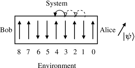
Figure 4: Schematic drawing of the teleportation procedure that we study in the text. Alice sends one of the qubits of her pure Bell state to Bob. Meanwhile there is dissipation induced by the environment. In the figure, there is a chain of $n=9$ qubits and the third of the $n-2$ swap gates required by this quantum protocol has been applied. Qubit $|\psi\rangle$ has to be teleported.

Let us first recall this protocol in the ideal case, without environmental effects. We consider a chain of $n$ qubits, and assume that Alice can access the qubits located at one end of the chain, Bob those at the other end. Initially Alice owns an EPR pair (for instance we take the Bell state $|\phi^{+}\rangle=(|00\rangle+|11\rangle)/\sqrt{2}$), while the remaining $n-2$ qubits are in a pure state. Thus, the global initial state of the chain is given by

$$\sum_{i_{n-1},\ldots,i_{2}}c_{i_{n-1},\ldots,i_{2}}|i_{n-1}\ldots i_{2}\rangle\otimes\frac{1}{\sqrt{2}}(|00\rangle+|11\rangle),$$ (30)

where $i_{k}=0,1$ denotes the up or down state of the qubit $k$. In order to deliver one of the qubits of the EPR pair to Bob, we implement a protocol consisting of $n-2$ swap gates that exchange the states of pairs of qubits:

$$\sum_{i_{n-1},\ldots,i_{2}}\frac{c_{i_{n-1},\ldots,i_{2}}}{\sqrt{2}}(|i_{n-1}\ldots i_{2}00\rangle+|i_{n-1}\ldots i_{2}11\rangle)$$

$$\rightarrow\sum_{i_{n-1},\ldots,i_{2}}\frac{c_{i_{n-1},\ldots,i_{2}}}{\sqrt{2}}(|i_{n-1}\ldots 0i_{2}0\rangle+|i_{n-1}\ldots 1i_{2}1\rangle)\rightarrow$$

$$...\rightarrow\sum_{i_{n-1},\ldots,i_{2}}\frac{c_{i_{n-1},\ldots,i_{2}}}{\sqrt{2}}(|0i_{n-1}\ldots i_{2}0\rangle+|1i_{n-1}\ldots i_{2}1\rangle).$$ (31)

After that, Alice and Bob share an EPR pair, and therefore an unknown state of a qubit ($|\psi\rangle=a|0\rangle+b|1\rangle$) can be transferred from Alice to Bob by means of the standard teleportation protocol BennettBrassard . In this work, we take random coefficients $c_{i_{n-1},\ldots,i_{2}}$, that is they have amplitudes of the order of $1/\sqrt{2^{n-2}}$ (to assure wave function normalization) and random phases. This ergodic hypothesis models the transmission of a qubit through a chaotic quantum channel.

We assume that our quantum protocol is implemented by a sequence of instantaneous and perfect swap gates, separated by a time interval $\tau$, during which the corresponding noise channels introduce errors. This means that, using quantum trajectories, dissipation is implemented by means of “infinitesimal” Kraus operators (see Sec. III), following the quantum jump numerical procedure outlined in Sec. II.1. We also assume that the only effect of the system’s Hamiltonian $H_{s}$ is to generate the swap gates.

Let us call $\rho_{k}^{(n)}$ the density matrix of the whole chain of $n$ qubits after $k$ swap gates. Since the evolution of the density matrix in a time step $dt$ is given, in the Kraus representation, by Eq. (11), we can write the evolution from $\rho_{k-1}^{(n)}$ to $\rho_{k}^{(n)}$ as follows:

$$\rho_{k}^{(n)}=U_{\rm sw}^{k,k+1}\>\left[\sum_{\mu_{1},...,\mu_{k}=0}^{\cal M}M_{\mu_{k}}^{(n)}(dt)\cdots M_{\mu_{1}}^{(n)}(dt)\right.$$

$$\rho_{k-1}^{(n)}\>\left.(M_{\mu_{1}}^{(n)})^{\dagger}(dt)\cdots(M_{\mu_{k}}^{(n)})^{\dagger}(dt)\right]\>{U_{\rm sw}^{k,k+1}}^{{\dagger}},$$ (32)

where $U_{\rm sw}^{ij}$ is the swap operator that exchanges the states of the qubits $i$ and $j$ and $k=\tau/dt$ is the number of quantum noise operations between two consecutive swap gates. After $n-2$ swap gates, we obtain the final state $\rho_{f}^{(n)}=\rho_{n-2}^{(n)}$.

After computing the evolution of the initial state of the chain of $n$ qubits up to time $\Delta t=(n-2)\tau$, the standard teleportation protocol is implemented BennettBrassard . The fidelity of teleportation is defined by

$$F=\langle\psi|\rho_{B}|\psi\rangle,$$ (33)

where $|\psi\rangle=a|0\rangle+b|1\rangle$ is the state to be teleported, and $\rho_{B}$ is the density matrix of Bob’s qubit at the end of the teleportation protocol, obtained after tracing over all the other qubits of the chain: $\rho_{B}={\rm Tr}_{0,...,n-2}[\rho_{f}^{(n)}]$.

In the quantum trajectories method, we compute the fidelity as

$$F=\lim_{{\cal N}\to\infty}\frac{1}{\cal N}\sum_{i=1}^{\cal N}\langle\psi|(\rho_{B})_{i}|\psi\rangle,$$ (34)

where $(\rho_{B})_{i}$ is the reduced density matrix of Bob’s qubit, obtained from the wave vector of the trajectory $i$ at the end of the quantum protocol. If the final state of the chain is $|\phi\rangle=\sum_{j=0}^{2^{n}-1}\alpha_{j}|j\rangle$ (an arbitrary state), the state of the whole system is

$$|\phi\rangle|\psi\rangle= \frac{1}{\sqrt{2}}\sum_{j^{\prime}=0}^{2^{n-1}-1}[(a\alpha_{2j^{\prime}}+b\alpha_{2j^{\prime}+1})|j^{\prime}\rangle|\phi^{+}\rangle$$ (35)

$$+(a\alpha_{2j^{\prime}}-b\alpha_{2j^{\prime}+1})|j^{\prime}\rangle|\phi^{-}\rangle.$$

$$+(b\alpha_{2j^{\prime}}+a\alpha_{2j^{\prime}+1})|j^{\prime}\rangle|\psi^{+}\rangle$$

$$+(b\alpha_{2j^{\prime}}-a\alpha_{2j^{\prime}+1})|j^{\prime}\rangle|\psi^{-}\rangle],$$

In the previous expression we have used the four (maximally entangled) Bell states ($|\phi^{\pm}\rangle=(|00\rangle\pm|11\rangle)/\sqrt{2}$ and $|\psi^{\pm}\rangle=(|01\rangle\pm|10\rangle)\sqrt{2}$), corresponding to the two least significant bits (the first bit of the chain and $|\psi\rangle$). Then, as required by the teleportation protocol, we perform a Bell measurement whose result determines one out of possible unitary transformations acting on Bob’s qubit. Owing to quantum noise, Bob’s qubit is entangled with the rest of the chain. Therefore, we must trace over these qubits to obtain the reduced density matrix $\rho_{B}$ describing the state of Bob’s qubit. If we measure $|\phi^{+}\rangle$ for instance, and define $\tilde{\alpha}_{j^{\prime}}=1/\sqrt{2}\>(a\;\alpha_{2j^{\prime}}+b\;\alpha_{2j^{\prime}+1})$, we arrive at the following expression:

$$\rho_{\rm B}=C\left(\begin{array}[]{ll}\sum_{j^{\prime}=0}^{D-1}|\tilde{\alpha}_{j^{\prime}}|^{2}&\sum_{j^{\prime}=0}^{D-1}\tilde{\alpha}_{j^{\prime}}\tilde{\alpha}_{j^{\prime}+D}^{*}\\ \sum_{j^{\prime}=0}^{D-1}\tilde{\alpha}_{j^{\prime}}^{*}\tilde{\alpha}_{j^{\prime}+D}&\sum_{j^{\prime}=D}^{2D-1}|\tilde{\alpha}_{j^{\prime}}|^{2}\end{array}\right),$$ (36)

where $D=2^{n-2}$ and $C=1/\sum_{j^{\prime}=0}^{2D-1}|\tilde{\alpha}_{j^{\prime}}|^{2}$ is a normalization constant. Then, the fidelity becomes

$$F= C\big{(}|a|^{2}\sum_{j^{\prime}=0}^{D-1}|\tilde{\alpha}_{j^{\prime}}|^{2}+|b|^{2}\sum_{j^{\prime}=D}^{2D-1}|\tilde{\alpha}_{j^{\prime}}|^{2}+$$ (37)

$$+\sum_{j^{\prime}=0}^{D-1}2\text{Re}(\tilde{\alpha}_{j^{\prime}}\tilde{\alpha}_{j^{\prime}+D}^{*}a^{*}b)\big{)}.$$

In the special case $a=b=1/\sqrt{2}$, it reduces to

$$F=\frac{1}{2}+C\sum_{j^{\prime}=0}^{D-1}\text{Re}(\tilde{\alpha}_{j^{\prime}}\tilde{\alpha}_{j^{\prime}+D}^{*}).$$ (38)

Similar expressions are obtained when the Bell measurement gives outcomes $|\phi^{-}\rangle$, $|\psi^{+}\rangle$, or $|\psi^{-}\rangle$.

Let us now briefly discuss the case in which we directly evolve the density matrix of the whole system by means of the master equation (3). After the sequence of swap gates and quantum noise operations, we obtain the final density matrix $\rho_{f}^{(n)}$ for the $n$-qubit chain. The Bell measurement is performed by the operator

$$\frac{M_{\phi^{+}}(\rho_{f}^{(n)}\otimes\rho_{\psi})M_{\phi^{+}}^{{\dagger}}}{{\rm Tr}[M_{\phi^{+}}(\rho_{f}^{(n)}\otimes\rho_{\psi})M_{\phi^{+}}^{{\dagger}}]},$$ (39)

where $\rho_{\psi}=|\psi\rangle\langle\psi|$ is the density matrix describing the state of the qubit to be teleported and $M_{\phi^{+}}=\openone^{(n-1)}\otimes|\phi^{+}\rangle\langle\phi^{+}|$ ($\openone^{(n-1)}$ is the identity for the remaining $n-1$ qubits of the chain). Then, we take the partial trace and obtain the fidelity $F={\rm Tr}(\rho_{\rm B}\rho_{\psi})=\langle\psi|\rho_{\rm B}|\psi\rangle$. It is straightforward to see that the above procedure is equivalent to take the partial trace (over the mediating qubits of the chain) first and then proceed with low dimensionality calculations.

We have investigated the effect of the two amplitude damping models described in Sec. III on the fidelity of quantum teleportation. In Fig. 5, we show the results of our numerical simulations for the special case in which the state to be teleported is $|\psi\rangle=(|0\rangle+|1\rangle)/\sqrt{2}$. In this case, in the limit of infinite chain ($n\to\infty$) or of large damping rate, the density matrix $\rho_{\rm B}$ describing the state of Bob’s qubit becomes $\rho_{\rm B}=|0\rangle\langle 0|$. Thus, the asymptotic value of fidelity is given by $F_{\infty}=1/2$ and we plot the values of $\bar{F}=F-F_{\infty}$, for the noise models (17) and (23), corresponding to the inset and the main figure in Fig. 5, respectively. For both cases we have checked the accuracy of the quantum trajectory simulations by reproducing the results with direct density matrix calculations. This was possible only up to $n=10$ qubits. The exponential decay of fidelity in the case in which quantum noise is modeled by Eq. (23) is in agreement with the theoretical formula

$$F=\frac{1}{2}+\frac{1}{2}\exp{\left(-\frac{\Gamma t}{\hbar}\right)}=\frac{1}{2}+\frac{1}{2}\exp(-\gamma k),$$ (40)

where $\gamma=\Gamma\tau/\hbar$ is the dimensionless damping rate and $k=t/\tau=n-2$ measures the time in units of quantum (swap) gates. To derive this theoretical formula, we observe that this quantum noise model does not generate entanglement between the two qubits of the Bell pair and the others qubit of the chain. Therefore, it is sufficient to study the evolution of the Bell state $|\phi^{+}\rangle\langle\phi^{+}|$ under the noise model (23). This evolution takes place inside a two-qubit Hilbert space of dimension $4$ and its exact solution is given by Eq. (40). On the contrary, the quantum noise model (17) entangles these two qubits with the rest of the chain. In this case, the fidelity decay is not exponential. Unfortunately, we could not provide an analytical derivation of $F(t)$ in this case.

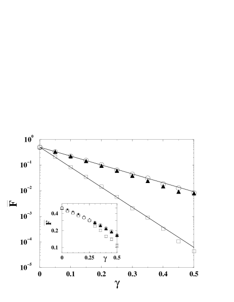
Figure 5: Fidelity $\bar{F}=F-F_{\infty}$ ($F_{\infty}=1/2$) of the teleportation of the state $|\psi\rangle=(|0\rangle+|1\rangle)/\sqrt{2}$ as a function of the dimensionless damping rate $\gamma=\Gamma\tau/\hbar$, for the amplitude damping model (23). Circles and squares are the results of the quantum trajectories calculations for chains with $n=10$ and $n=20$ qubits, respectively. Triangles give the results of the density matrix calculations at $n=10$. Straight lines correspond to the theoretical result of Eq. (40). Inset: the same but for the noise model (17).

V The quantum baker’s map

The quantum algorithm for the simulation of the quantum baker’s map has been proposed by Schack Sch and recently implemented by means of a three-qubit NMR-based quantum processor cory , where the fidelity of the quantum computation of the baker’s map in one map step was measured.

The baker’s transformation is one of the prototype models of classical and quantum chaos Bala . It maps the unit square $0\leq{q,p}<1$ onto itself according to

$$q_{k+1} = 2q_{k}-[2q_{k}],$$

$$p_{k+1} = (p_{k}+[2q_{k}])/2,$$ (41)

where $[x]$ stands for the integer part of $x$ and the index $k$ denotes the number of map iterations. The action of this map corresponds to compressing the unit square in the $p$ direction and stretching it in the $q$ direction, then cutting it along the $p$ direction, and finally stacking one piece on top of the other (similarly to the way a baker kneads dough). Note that map (41) is area preserving. The baker’s map is a paradigmatic model of classical chaos. Indeed, it exhibits sensitive dependence on initial conditions, which is the distinctive feature of classical chaos: any small error in determining the initial conditions is amplified exponentially in time. In other words, two nearby trajectories separate exponentially, with a rate given by the maximum Lyapunov exponent $\lambda=\ln 2$.

The baker’s map can be quantized following Bala . We introduce the position ($q$) and momentum ($p$) operators, and denote the eigenstates of these operators by $|q_{j}\rangle$ and $|p_{k}\rangle$, respectively. The corresponding eigenvalues are given by $q_{j}=j/N$ and $p_{k}=k/N$, with $j,k=0,\dots,N-1$, $N$ being the dimension of the Hilbert space. Note that, to fit $N$ levels onto the unit square, we must set $2\pi\hbar=1/N$. Therefore, the effective Planck’s constant of the system is $\hbar_{\rm eff}\propto 1/N$. We take $N=2^{n}$, where $n$ is the number of qubits used to simulate the quantum baker’s map on a quantum computer. Note that $\hbar_{\rm eff}$ drops exponentially with the number of qubits and therefore the semiclassical regime $\hbar_{\rm eff}\ll 1$ can be reached with a small number of qubits. The transformation between the position basis $\{|q_{0}\rangle,\dots,|q_{N-1}\rangle\}$ and the momentum basis $\{|p_{0}\rangle,\dots,|p_{N-1}\rangle\}$ is performed by means of a discrete Fourier transform $F_{n}$, defined by the matrix elements

$$\langle q_{k}|F_{n}|q_{j}\rangle\equiv\frac{1}{\sqrt{2^{n}}}\,\exp\!\left(\frac{2\pi ikj}{2^{n}}\right).$$ (42)

It can be shown Bala that the quantized baker’s map may be defined by the transformation

$$|\psi_{k+1}\rangle=B\,|\psi_{k}\rangle=F_{n}^{-1}\left[\begin{array}[]{cc}F_{n-1}&0\\ 0&F_{n-1}\end{array}\right]|\psi_{k}\rangle,$$ (43)

where $|\psi_{k}\rangle$ denotes the wave vector of the system after $k$ map steps, the matrix elements are to be understood relative to the position basis $\{|q_{j}\rangle\}$ and $F_{n-1}$ is the discrete Fourier transform, defined by Eq. (42).

Since the discrete Fourier transform can be calculated on a quantum computer using $O(n^{2})$ elementary gates (see, e.g., Ref. Chuangbook ), the simulation of one step of the baker’s map requires $O(n^{2}=(\log N)^{2})$ gates Sch (more precisely, we need $(n-1)^{2}$ controlled phase-shift gates and $2n-1$ Hadamard gates). Therefore, it is exponentially faster than the best known classical computation, which is based on the fast Fourier transform and requires $O(N\log N)$ gates.

In this section, we investigate the fidelity of the quantum computation of the baker’s map in the presence of quantum noise. We consider the phase flip noise channel, generalized to the $n$-qubit case as discussed in Sec. III. We take an initial state $|\psi_{0}\rangle$ with amplitudes of the order of $1/\sqrt{2^{n}}$ and random phases. We perform the forward evolution of the baker’s map up to time $k$ (this evolution is driven, in the noiseless case, by the unitary operator $B^{k}$, with $B$ given in Eq. 43), followed by the $k$-step backward evolution (represented by the operator $(B^{\dagger})^{k}$). Due to quantum noise, the initial state $|\psi_{0}\rangle$ is not exactly recovered and the final state of the system is described by a density matrix $\rho_{f}$. The fidelity of quantum computation is given by $F=\langle\psi_{0}|\rho_{f}|\psi_{0}\rangle$.

We are able to work out the following theoretical formula for the decay of fidelity induced by phase flip noise:

$$F=\exp\left(-n\gamma N_{g}\right)=\exp(-2\gamma n^{3}k),$$ (44)

where $\gamma=\Gamma\tau/\hbar$ is the dimensionless decay rate (again, $\tau$ denotes the time interval between elementary quantum gates) and $N_{g}=2n^{2}k$ is the total number of elementary quantum gates required to implement the $k$ steps forward evolution of the baker’s map, followed by $k$ step backward. To derive this formula, we first of all note that Eq. (29), obtained in the absence of any quantum gate operation, gives, at short times, the exponential decay

$$F(t)=\exp(-\frac{<\Gamma>t}{\hbar}).$$ (45)

Here the decay rate $<\Gamma>$ is obtained after averaging all the decay rates that appear in Eq. (29):

$$<\Gamma>=\frac{n!}{2^{n}}\>\sum_{i=0}^{n}\frac{1}{i!\>(n-i)!}2i\Gamma=n\Gamma.$$ (46)

The effect of the chaotic dynamics of the baker’s map is to induce a fast decay of correlations, so that any memory of the initial state is rapidly lost and the fidelity decay remains exponential also at long times. Therefore, the condition for the validity of formula (44) is that the randomization process introduced by chaotic dynamics takes place in a time scale shorter than the time scale for fidelity decay.

We can determine from Eq. (44) the time scale up to which a reliable quantum computation of the baker’s map evolution in the presence of the phase flip noise channel is possible even without quantum error correction. The time scale $k_{f}$ at which $F$ drops below some constant $A$ (for instance, $A=0.9$) is given by

$$k_{f}=-\frac{\ln A}{2\gamma n^{3}}.$$ (47)

The total number of gates that can be implemented up to this time scale is given by

$$(N_{g})_{f}=2n^{2}k_{f}=-\frac{\ln A}{\gamma n}.$$ (48)

Our theoretical expectations are confirmed by the numerical data of Figs. 6 and 7. In Fig. 6, we show the fidelity after one map step, as a function of the dimensionless damping rate $\gamma=\Gamma\tau/\hbar$. The numerical data of this figure show that the fidelity drops exponentially with $\gamma$, in excellent agreement with Eq. (44). We point out that our theory predicts not only the exponential fidelity decay but also the numerical value of the decay rate. Finally, we show in Fig. 7 the number $k_{f}$ of forward/backward map steps required to reach a fixed value $A$ of the fidelity ($F=A=0.9$), as a function of the number $n$ of qubits. This time scale decays as a power law, $k_{f}=C/n^{3}$, in agreement with Eq. (44). Again, our theory predicts also the value of the prefactor $C$, in excellent agreement with numerical data.

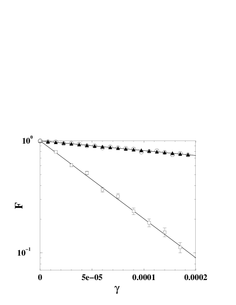
Figure 6: Semi log plot of the fidelity as a function of the dimensionless decay rate $\gamma$, for the baker’s map after one map step in the presence of the phase flip channel described in the text. Circles and squares correspond to quantum trajectories simulations with ${\cal N}=500$ trajectories, at $n=10$ and $n=20$ qubits, respectively. Triangles give the results obtained by direct computation of the density matrix evolution at $n=10$. Solid lines stand for the theoretical prediction of Eq. (44), namely $F(\gamma)=\exp(-2\gamma n^{3})$.

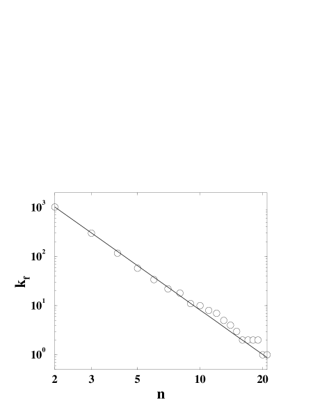
Figure 7: Logarithmic plot of the time scale $k_{f}$ (measured in number of steps of the baker’s map) required to reach a fidelity value of $F=0.9$, as a function of the number $n$ of qubits, for $\gamma\approx 6.47\times 10^{-5}$ (this value has been chosen by demanding that $F=0.9$ after one forward/backward step of the baker’s map at $n=21$). The straight line gives the theoretical curve $T(n)=C/n^{3}$, with $C=-\ln(0.9)/(2\gamma)\approx 8.14$.

As we have seen above, the number of gates that can be reliably implemented without quantum error correction drops only polynomially with the number of qubits, $(N_{g})_{f}\propto 1/n$ (see Eq. 48). We would like to stress that this dependence should remain valid also in other environment models that allow only one qubit at a time to perform a transition, like the other noise channels descussed in Sec. III. Furthermore, we note that the time scales for fidelity decay derived in this section and confirmed in the baker’s map model, are expected to be valid for any quantum algorithm simulating dynamical systems in the regime of quantum chaos.

VI Conclusion

We have studied two quantum protocols, i.e. a teleportation scheme through a chain of qubits and a quantum algorithm for the quantum baker’s map. We have modeled different sorts of environments in order to get a deeper insight of the stability of quantum computation when different interactions with the environment taken into account. Two kinds of generalized amplitude damping models have been considered for the teleportation scheme, giving very different behaviors. After a theoretical analysis we were able to understand the origin of these differences. This reveals the importance of the details of the environmental models in assessing the operability bounds of quantum processors. In the case of the baker’s map simulation, we have chosen the phase flip type of noise and we could verify our theoretical predictions for fidelity decay. The results of this paper show that quantum trajectories are a very valuable tool for simulating noise processes in quantum information protocols with a high degree of efficiency.

- (1) W.H. Zurek, Rev. Mod. Phys. 75, 715 (2003).
- (2) H. Grabert, P. Schramm, and G.-L. Ingold, Phys. Rep. 168, 115 (1988).
- (3) T. Dittrich, P. Hänggi, G.-L. Ingold, B. Kramer, G. Schön, and W. Zwerger, Quantum transport and dissipation (Wiley, Weinheim, 1998).
- (4) M.B. Plenio and P.L. Knight, Rev. Mod. Phys. 70, 101 (1998).
- (5) P.W. Shor, SIAM J. Sci. Statist. Comput., 26, 1484 (1997).
- (6) R. Schack, Phys. Rev. A 57, 1634 (1998).
- (7) B. Georgeot and D.L. Shepelyansky, Phys. Rev. Lett. 86, 2890 (2001).
- (8) G. Benenti, G. Casati, S. Montangero, and D.L. Shepelyansky, Phys. Rev. Lett. 87, 227901 (2001); Phys. Rev. A 67, 052312 (2003).
- (9) Y.S. Weinstein, S. Lloyd, J. Emerson, and D.G. Cory, Phys. Rev. Lett. 89, 157902 (2002).
- (10) R. Schack, T.A. Brun, and I.C. Percival, J. Phys. A 28, 5401 (1995).
- (11) A. Barenco, T.A. Brun, R. Schack, and T.P. Spiller, Phys. Rev. A 56, 1177 (1997).
- (12) G.G. Carlo, G. Benenti, and G. Casati, Phys. Rev. Lett. 91, 257903 (2003).
- (13) C.H. Bennett, G. Brassard, C. Crépeau, R. Jozsa, A. Peres, and W.K. Wootters, Phys. Rev. Lett. 70, 1895 (1993).
- (14) M.A. Nielsen and I.L. Chuang, Quantum Computation and Quantum Information (Cambridge University Press, Cambridge, 2000).
- (15) J. Preskill, Lecture notes on Quantum Information and Computation (available at www.theory.caltech.edu/people/preskill/ph229).
- (16) G. Lindblad, Commun. Math. Phys. 48, 119 (1976); V. Gorini, A. Kossakowski, and E.C.G. Sudarshan, J. Math. Phys. 17, 821 (1976).
- (17) J. Dalibard, Y. Castin, and K. Mølmer, Phys. Rev. Lett. 68, 580 (1992).
- (18) T.A. Brun, Am. J. Phys. 70, 719 (2002); T. A. Brun, quant-ph/0301046.
- (19) W.H. Zurek, Phys. Today, October 1991, 36 (1991); see also quant-ph/0306072.
- (20) N. Gisin and I.C. Percival, J. Phys. A 25, 5677 (1992).
- (21) V.V. Flambaum and F.M. Izrailev, Phys. Rev E 64, 036220 (2001).
- (22) P. Badziag, M. Horodecki, P. Horodecki, and R. Horodecki, Phys. Rev. A 62, 012311 (2000).
- (23) S. Bandyopadhyay, Phys. Rev A 65, 022302 (2002).
- (24) S. Oh, S. Lee, and H-w Lee, Phys. Rev. A 66, 022316 (2002).
- (25) F. Verstraete and H. Verschelde, Phys. Rev. Lett 90, 097901 (2003).
- (26) N.L. Balazs and A. Voros, Ann. Phys. (N.Y.) 190, 1 (1989); M. Saraceno and A. Voros, Physica D 79, 206 (1994).