Quantum linear mutual information and classical correlations in globally pure bipartite systems

Abstract

We investigate the correlations of initially separable probability distributions in a globally pure bipartite system with two degrees of freedom for classical and quantum systems. A classical version of the quantum linear mutual information is introduced and the two quantities are compared for a system of oscillators coupled with both linear and non-linear interactions. The classical correlations help to understand how much of the quantum loss of purity are due to intrinsic quantum effects and how much is related to the probabilistic character of the initial states, a characteristic shared by both the classical and quantum pictures. Our examples show that, for initially localized Gaussian states, the classical statistical mutual linear entropy follows its quantum counterpart for short times. For non-Gaussian states the behavior of the classical and quantum measures of information are still qualitatively similar, although the fingerprints of the non-classical nature of the initial state can be observed in their different amplitudes of oscillation.

I Introduction

Entanglement has been a focus of intense investigation in the recent years due to its relevance in quantum computation and quantum information 1 ; 2 ; vedral ; plenio ; vidal ; woot . From a fundamental point of view, entanglement is considered “the characteristic trait of quantum mechanics, the one that enforces its entire departure from classical lines of thought” (Schrödinger)schrodinger35 . Entanglement reflects quantum correlations in the Hilbert space, where state vectors are associated with probability distributions. In classical mechanics, on the other hand, states are described by points in phase space, and no intrinsic probabilistic character exists.

Probability distributions can be introduced in classical mechanics with the Liouville formalism, and statistical averages on ensembles can be calculated. Initially independent probability distributions can become correlated when evolved by a classical Hamiltonian with interaction terms. These correlations represent the dynamical emergence of conditional probabilities in the classical statistical world.

In this paper we consider the time evolution of a bipartite system whose Hilbert space is the direct product of two subspaces. Initial states that are the tensor product of kets in each subspace, usually evolve to non-product states, generating coherences and entangling the two subsystems. A measure of the non-separability between them is provided either by the Von Neumann or the linear entropies. In the case of a globally pure bipartite system we argue that the latter is a convenient quantum measure of non-separability. Next, as the main point of our work, we consider the time evolution of probability densities in the phase space of the corresponding bipartite classical analogue. Inspired on the quantum problem we propose a measure of the classical correlations generated by the statistical ensembles of classical trajectories. We want to measure the non-separability of the classical probability distribution evolving in time via Liouville equations. Moreover we want to compare behavior of this classical measure with the loss of purity of the quantum system, particularly at short times. This comparison helps to identify the time at which intrinsic quantum effects, such as interferences, begin to be important.

In our approach we first define a classical statistical quantity and compare its behavior with the quantum linear entropy (QLE). Due to its formal similarity with the quantum linear entropy, we call it classical statistical linear entropy (CSLE). A similar classical quantity has recently been used in the study of quantum-classical correspondence of intrinsic decoherence gong03 . In spite of the direct correspondence between the QLE and the CSLE, the latter may not be symmetric between the two subsystems that make up the global bipartite system, i.e., the CSLE of each subspace does not contain in general the same information. Also, the CSLE can assume negative values and is restricted to initially separable distributions, not being a good measure in the case of distributions that start off non-separable. We therefore define a more general classical measure, the classical statistical linear mutual information (CSLMI), based on the concept of quantum mutual information (QMI) vedral97 , that is always symmetric and positive, and thus, best suited to measure the classical separability. We show that for two bi-linearly coupled harmonic oscillators with Gaussian initial distributions, the classical and quantum results coincide. For non-linear coupling the classical and quantum entropies remain close for short times for both regular and chaotic regimes.

The outline of this work is as follows. In Section II.A we give some general definitions and show that the quantum linear entropy can be expressed in terms of the non-diagonal terms of the density operator, providing a good measure of the entanglement between the subsystems. In Section II.B we present our definitions of the classical statistical linear entropy with some considerations about the initial probability distributions. Next we introduce the quantum linear mutual information and its classical statistical analogue. This allows us to treat cases where the two subsystems have different types of initial distributions in phase space. Section III is reserved to the comparison between the QLMI and the CSLMI for a system of two oscillators coupled with the following types of interactions: (1) bi-linear; (2) non-linear ; (3) bilinear within the rotating wave approximation (RWA). As initial states we consider both Gaussian and non-Gaussian distributions. Finally in Section IV we present some conclusions and discuss the adequacy and limitations of the present approach.

II Theory

II.1 Quantum Linear Entropy

The density operator corresponding to an initially (normalized) pure state $|\psi_{0}\rangle$ is

$$\rho(t)=U(t)\,|\psi_{0}\rangle\langle\psi_{0}|\,U^{\dagger}(t),$$ (1)

where $U(t)=e^{-iHt/\hbar}$ is the evolution operator and $H$ is the Hamiltonian. For a globally pure state, there are constraints connecting the diagonal and off-diagonal matrix elements of the density operator. This follows from the property $Tr\rho^{2}=Tr\rho=1$, which can be written explicitly as

$$\sum_{i}\rho_{ii}{{}^{2}}+\sum_{i}\sum\limits_{k\neq i}|\rho_{ik}|^{2}=\sum_{i}\rho_{ii}=1\;,$$ (2)

where we have separated the diagonal and off-diagonal terms in the left hand side. From this relation we define

$$d(\rho)\equiv\sum_{i}\sum\limits_{k\neq i}|\rho_{ik}|{{}^{2}}=1-\sum_{i}\rho_{ii}{{}^{2}}\;.$$ (3)

Consider now a bipartite system whose Hilbert space is the direct product of two sub-spaces: $\mathcal{E}=\mathcal{E}_{1}\otimes\mathcal{E}_{2}$. A measure of non-separability between these subsystems for a globally pure state is provided either by the Von Neumann or by the linear entropies vedral97 ; manfredi . The partial trace of $\rho$ on system $2$ defines the operator

$$\rho_{1}(t)=tr_{2}(\rho(t))\;.$$ (4)

The corresponding QLE is given by

$$S_{1}(t)=1-tr_{1}(\rho_{1}^{2}(t))\;.$$ (5)

The operator $\rho_{2}(t)$ and the QLE $S_{2}(t)$ are similarly defined.

For $H=H_{1}\otimes\mathbf{1}_{2}+\mathbf{1}_{1}\otimes H_{2}$ both $\rho_{1}(t)$ and $\rho_{2}(t)$ are projectors and $S_{1}(t)=S_{2}(t)=0$. If couplings between the sub-spaces exist, they force the global state to evolve to non-product states, entangling the subsystems and producing non-zero values for $S_{1}(t)$ and $S_{2}(t)$.

In fact, for a globally pure bipartite system $S_{1}=S_{2}=d(\rho)$. To see this we write

$$|\psi\rangle=\sum_{i}\lambda_{i}|a_{i}\rangle|b_{i}\rangle,$$ (6)

where $\{|a_{i}\rangle\}$ and $\{|b_{i}\rangle\}$ are orthonormal basis of subsystems $1$ and $2$ respectively, and $\{\lambda_{i}\}$ is the Schmidt spectrum schmidt07 . Then,

$$\rho=\sum_{i,j}\rho_{ij}|a_{i}\rangle|b_{i}\rangle\langle a_{j}|\langle b_{j}|,$$ (7)

with $\rho_{ij}=\lambda_{i}\lambda_{j}^{*}$. The reduced density of system $1$ becomes

$$\rho_{1} = \sum_{i}\rho_{ii}|a_{i}\rangle\langle a_{i}|,$$ (8)

and similarly for system $2$. The subsystem linear entropy becomes trivial in this basis:

$$S_{1}=1-Tr_{1}(\rho_{1}^{2})=1-\sum_{i}\rho_{ii}^{2}$$ (9)

with a similar result for $S_{2}$.

Comparing this result with Eq.(3) we see that

$$S_{1}=S_{2}=\sum_{i}\sum\limits_{k\neq i}|\rho_{ik}|^{2}=d(\rho).$$ (10)

Therefore, as long as any globally pure state of the system can be decomposed in the Schmidt basis, we can conclude that the linear entropy indeed measures coherences between the subsystems. Furthermore, because of the total conservation of coherences (2), the linear entropy seems to be the most natural measure in the present situation.

II.2 Classical Systems

A measure of non-separability for classical systems can be defined only at a statistical level by considering ensembles of initial conditions 3 ; 4 ; 5 . Following Wehrl wehrl we define a quantity that we call classical statistical linear entropy.

Consider a system with two degrees of freedom described by the classical Hamiltonian function $\cal{H}$. Consider also several copies of this system with initial conditions distributed according to the ensemble probability distribution $P(x,t=0)$, where $x\equiv(q_{1},p_{1},q_{2},p_{2})$. The classical time evolution of $P(x,0)$ is obtained via Liouville’s equation

$$\frac{\partial P}{\partial t}=\{\mathcal{H},P\},$$ (11)

whose solution is

$$P(x,t)=P(\phi_{t}^{-1}(x),0),$$ (12)

where $\phi_{t}^{-1}(x)\equiv x_{0}$ is the initial condition that propagates to $x$ in the time $t$ and $\phi_{t}$ is the phase space flux, so that $x=\phi_{t}(x_{0})$. In words, the numerical value of the probability $P$ at point $x$ and time $t$ has the same numerical value of the probability at point $x_{0}$ of the initial distribution. This value is carried over to $x$ in the time $t$. Liouville’s theorem guarantees the conservation of probability at all times. For integrable systems $\phi_{t}(x_{0})$ might be determined analytically, otherwise numerical calculations can be performed. Notice that $P(x,t)$ is itself a constant of motion, but this is not enough to guarantee the integrability of the system, since it is not generally in involution with the Hamiltonian.

The marginal probability distribution

$$P_{1}(q_{1},p_{1},t)=\int dq_{2}dp_{2}P(q_{1},p_{1},q_{2},p_{2},t)$$ (13)

allows us to define the classical statistical linear entropy

$$S_{1}^{cl}(t)=1-\frac{\int dq_{1}dp_{1}P_{1}^{2}(q_{1},p_{1},t)}{\int dq_{1}dp_{1}P_{1}^{2}(q_{1},p_{1},0)}\;.$$ (14)

The normalization is necessary for dimensional reasons and to guarantee that $S_{1}^{cl}(0)=0$.

The initial classical distribution corresponding to a given quantum pure state $\rho(0)$ is chosen as the coherent states phase space projection

$$P(x,0)=\frac{1}{N}\langle\alpha_{1},\alpha_{2}|\rho(0)|\alpha_{2},\alpha_{1}\rangle,$$ (15)

where $N$ is a normalization constant and $\alpha_{i}=(q_{i}+\imath p_{i})/\sqrt{2\hbar}$ is the usual complex parametrization of the coherent states. Eq. (15) is the normalized Husimi distribution, which is positive definite by construction. It is known that the Husimi distribution does not reproduce the correct marginal probabilities. However, the constraint of a positive probability distribution excludes the Wigner function 6b as a classical initial distribution.

Eqs.(3) and (10) show that the quantum linear entropies $S_{1}$ and $S_{2}$ can be obtained only from the diagonal elements of the global density matrix. Diagonal elements, on the other hand, have classical analogues. Therefore it makes sense to compare the dynamics of $S_{1}$ and $S_{2}$, which may be written either in terms of only off-diagonal or only diagonal elements, with the classical correlations.

An important difference between the classical and quantum linear entropies can be made explicit in the coherent state basis. For one dimensional systems we obtain

$$S(t)=1-\int\frac{d{{}^{2}}\alpha}{\pi}\Big{[}\langle\alpha|U(t)\rho{{}^{2}}(0)U^{{\dagger}}(t)|\alpha\rangle\Big{]}.$$ (16)

On the other hand, defining the Liouvillian operator $\cal{L}$ such that $\{\mathcal{H},P\}=\mathcal{L}P$, Eq.(11) can be formally integrated and the CSLE can be written as

$$S^{cl}(t)=1-\int\frac{d{{}^{2}}\alpha}{\pi}\left[\frac{\left(e^{\mathcal{L}t}\langle\alpha|\rho(0)|\alpha\rangle\right)^{2}}{M}\right],$$ (17)

where $M=N{{}^{2}}/\pi$. In particular, at $t=0$ the integrand of the classical entropy depends on $\langle\alpha|\rho(0)|\alpha\rangle^{2}$ instead of $\langle\alpha|\rho^{2}(0)|\alpha\rangle$. Another important difference is of course in the dynamics: the quantum evolution is determined by non-commuting operators, which brings a number of corrections to the classical formalism. For more degrees of freedom, although the time evolution cannot be expressed in such a simple way, the two differences pointed out above remain true.

II.3 Quantum and Classical Linear Mutual Information

Although the CSLE seems to be the natural classical analague of the quantum linear entropy, it is not symmetric between the subsystems. Indeed, if the initial probability distributions of each subsystem are not equal (for example a Gaussian distribution for one subsystem and a Poisonian distribution for the other) we find that $S_{1}^{cl}(t)\neq S_{2}^{cl}(t)$. The quantum linear entropy, on the other hand, always satisfies $S_{1}(t)=S_{2}(t)$. Another drawback of the definition Eq.(14) is that it gives $S_{1}^{cl}(0)=S_{2}^{cl}(0)=0$ for any initial classical distribution, correlated or not. Thus, it is interesting to define a more general quantity that avoids these difficulties and that takes into account the contributions of both subsystems entropies symmetrically. At the quantum level we define the quantum linear mutual information (QLMI) that depends on the QLE as $I\equiv S(\rho_{1}\otimes\rho_{2})-S(\rho)$. This is based on the Von Neumann mutual information vedral97 ; 11 , $I_{VN}=S_{VN}(\rho_{1}\otimes\rho_{2})-S_{VN}(\rho)$, where $S_{VN}$ is the Von Neumann entropy. By using Eq.(5) we can write the QLMI as (notice that the linear entropy is not additive manfredi )

$$I(t)=S_{1}(t)+S_{2}(t)-S_{1}(t)\,S_{2}(t)-S(t),$$ (18)

where $S_{i}$ and $S$ are the subsystem and the global linear entropies respectively. For pure initial states $S(t)=0$ and $I(t)=S_{1}+S_{2}-S_{1}S_{2}$.

We also define a quantity that we call classical statistical linear mutual information (CSLMI) as

$$I^{cl}(t)=S_{1}^{cl}(t)+S_{2}^{cl}(t)-S_{1}^{cl}(t)\,S_{2}^{cl}(t)-S^{cl}(t).$$ (19)

Once again $S^{cl}(t)=0$ for pure states. Note that the above definition can also be written in form $I^{cl}=S^{cl}(P_{1}\,P_{2})-S^{cl}(P)$ where $S^{cl}(P)$ is given by Eq.(14) with $P_{1}$ replaced by $P$.

We emphasize that the quantum and classical linear mutual information defined above are also non-separability measures, like the QLE and CSLE. This can be made explicit by re-writing Eqs.(18) and (19) as

$$I(t) = tr[\rho{{}^{2}}(t)-\rho_{1}{{}^{2}}(t)\otimes\rho_{2}{{}^{2}}(t)]$$ (20)

$$= 1-tr[\rho_{1}{{}^{2}}(t)\otimes\rho_{2}{{}^{2}}(t)],$$

$$I^{cl}(t) = \frac{\int dx[P{{}^{2}}(t)-P_{1}{{}^{2}}(t)P_{2}{{}^{2}}(t)]}{\int dxP{{}^{2}}(0)}$$ (21)

$$= 1-\frac{\int dxP_{1}{{}^{2}}(t)P_{2}{{}^{2}}(t)}{\int dxP{{}^{2}}(0)}.$$

The last equality is true since ${\int dxP^{2}(0)}={\int dxP^{2}(t)}$. When the two subsystems have the same type of initial distributions, both $I$ and $I^{cl}$ have the same contents of their respective linear entropies. Moreover, since $I^{cl}$ is symmetric with respect to the two subsystems, it does not present difficulties when the initial distributions are different.

In the next section we compare $I(t)$ with $I^{cl}(t)$ for three different cases.

III Results

In order to show that our definition of a CSLMI is physically sensible, we consider the following classical Hamiltonian with two degrees of freedom

$${\cal H}(q_{1},p_{1},q_{2},p_{2})={\cal H}_{1}+{\cal H}_{2}+{\cal H}_{I}\;,$$ (22)

where ${\cal H}_{i}=\frac{1}{2}(p_{i}^{2}+\omega_{i}^{2}q_{i}^{2})$ are harmonic oscillators and ${\cal H}_{I}$ is an interaction term. In what follows we shall calculate both CSLMI and QLMI for three different couplings: a simple bilinear, a non-integrable and a rotating-wave approximation (RWA). In the first and last cases the calculations can be performed analytically.

1) Bilinear Coupling ${\cal H}_{I}(q_{1},p_{1},q_{2},p_{2})=\lambda q_{1}q_{2}$ 7
In this case, the classical equations of motion can be easily integrated and we find

$$q_{1}(t)=q_{1}C_{+}(t)+q_{2}C_{-}(t)+p_{1}S_{+}(t)+p_{2}S_{-}(t),$$ (23)

$$p_{1}(t)=p_{1}C_{+}(t)+p_{2}C_{-}(t)-q_{1}S_{+}(t)-q_{2}S_{-}(t),$$

and similar expressions for $q_{2}(t)$ and $p_{2}(t)$. $C_{\pm}$ and $S_{\pm}$ are quasi-periodic functions of time

$$C_{\pm}(t)=\frac{1}{2}\left(\cos\Omega_{x}t\pm\cos\Omega_{y}t\right),$$

$$S_{\pm}(t)=-\frac{1}{2}\left({\Omega_{x}}\sin\Omega_{x}t\pm{\Omega_{y}}\sin\Omega_{y}t\right),$$ (24)

where $\Omega_{x}=\sqrt{\omega^{2}+\lambda}$ and $\Omega_{y}=\sqrt{\omega^{2}-\lambda}$.

As initial phase space distribution we choose a Gaussian centered at $x_{c}=(q_{1c},p_{1c},q_{2c},p_{2c})$,

$$P(x,0)=\frac{1}{4\pi{{}^{2}}\hbar{{}^{2}}}\exp\left\{-\frac{(x-x_{c})^{T}(x-x_{c})}{2\hbar}\right\}.$$ (25)

This is the classical density as given by Eq.(15), corresponding to a coherent state initial wave-function.

The probability distribution at time $t$ is obtained using Eqs. (12) and (23). The result can be written in the form

$$P(x,t)=\frac{1}{4\pi^{2}\hbar^{2}}e^{-x^{T}{\bf A}x+2Bx+C},$$ (26)

where the matrix ${\bf A}$ and the vector $B$ are functions of $C_{\pm}$, $S_{\pm}$ and $\hbar$. Replacing Eq.(26) into (19) we get

$$I^{cl}(t)=1-\frac{1}{64\hbar^{6}}\,\frac{1}{\det{(\beta)}^{2}\det{(\alpha-\gamma\beta^{-1}\gamma^{T})}},$$ (27)

where $\alpha$, $\beta$ and $\gamma$ are $2$ x $2$ matrices whose elements are combinations of $C_{\pm}$, $S_{\pm}$ and $T_{\pm}$, with

$$T_{\pm}(t)=-\left(\frac{\sin\Omega_{x}t}{\Omega_{x}}\pm\frac{\sin\Omega_{y}t}{\Omega_{y}}\right)\;.$$

It is interesting to note that all the dependence on the center position of the initial distribution has gone.

The reduced QLMI can also be analytically computed. Here, we simply write down the result:

$$I(t)=1-\left[\frac{4\hbar^{2}(1-\lambda^{2})}{|D_{x}(t)||D_{y}(t)|\,\sqrt{\det{(O)}}}\right]^{4}.$$ (28)

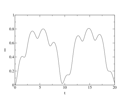
Figure 1: QLMI $I(t)$ and CSLMI $I_{cl}(t)$ as a function of time (arbitrary units) for the linear coupling and initial Gaussian distribution. The two curves are identical.

The coefficients $D_{i}(t)$ are periodic functions of frequency $\Omega_{i}$. $O$ is an $8\times 8$ quasi-periodic matrix depending on both $\Omega_{1}$ and $\Omega_{2}$. Expressions (27) and (28) are actually identical, which shows that our definition of $I^{cl}$ and the choice of its normalization are both appropriate. Fig. 1 displays an example for $\lambda=0.9$ that shows $I_{1}(t)=I_{1}^{cl}(t)$.

2) Nonlinear Coupling
The exact coincidence between the classical statistical and quantum linear mutual informations just presented, certainly has to do with both the quadratic nature of the Hamiltonian and the Gaussian initial distributions. To study the role of non-linearities we consider the interaction Hamiltonian

$${\cal H}_{I}(q_{1},p_{1},q_{2},p_{2})=-q_{1}p_{1}p_{2}+\frac{1}{2}{q_{1}}^{2}{q_{2}}^{2}.$$ (29)

The total Hamiltonian ${\cal H}$ is a canonically transformed version of a well studied system known as the Nelson potential 8 . Fig. 2 shows a typical mixed Poincaré section for parameter values $\omega_{1}=\sqrt{0.1}$, $\omega_{2}=\sqrt{2}$ and energy $E=0.05$.

The calculation of $I_{1}^{cl}(t)$ (Eq.(14)) now has to be performed numerically. We use the same initial distribution, Eq.(25). $x_{0}=\phi^{-1}_{t}(x)$ was calculated using standard Runge-Kutta routines. The integrations in Eqs.(13) and (14) was done both by Monte Carlo and by direct trapezoidal techniques; the results of the two methods agree in the time intervals we have considered. In Fig.(3a) we show $I(t)$ and the corresponding $I^{cl}(t)$. The initial density matrix is the direct product of two coherent states, and the initial classical probability distribution is that given by (15). The center of the coherent states is in the chaotic region of the corresponding Poincaré section. The resemblance between the QLMI and CSLMI is quite good even after two oscillations. Fig(3b) shows a similar calculation with the coherent states centered at the regular region. Once again the classical and quantum results coincide for short times. Surprisingly, the two entropy-like quantities agree for longer times in the chaotic case. For both the regular and chaotic cases, the classical and quantum calculations agree very well for short times, although the classical mutual information is systematically larger than its quantum counterpart for times larger than about $1$. Also, the linear mutual information grows faster for the chaotic case than for the regular case, in accordance with similar previous results for the linear entropy kyoko . Finally we note that the classical linear entropies Eq.(14) may become negative. Similar behaviors were reported in refs. wehrl ; manfredi . The linear mutual information, on the other hand, is always positive and better suited for measuring the classical loss of separability.

3) RWA Coupling: ${\cal H}_{I}(q_{1},p_{1},q_{2},p_{2})=\lambda(q_{1}q_{2}+p_{1}p_{2})$
This is the classical version of a rotating-wave approximation of the interaction Hamiltonian treated in the example (1). In this case, Gaussian distributions in each subspace evolve coherently: $I_{1}(t)=I_{1}^{cl}(t)=0$. However, this is a very particular case of a preferred basis state 6a ; 9 , and the same kind of coherent evolution is not expected for more general initial states. For instance, in the case of Fock states ($|\psi_{0}\rangle=|1\rangle\otimes|1\rangle$) the classical phase space distribution, given by the Husimi distribution, is

$$P(x,0)=\frac{e^{-\frac{(x-x_{c})^{T}(x-x_{c})}{2\hbar}}}{4\pi{{}^{2}}\hbar{{}^{2}}}\prod\limits_{k=1}^{2}\left(\frac{q_{k}{{}^{2}}+p_{k}{{}^{2}}}{2\hbar}\right).$$ (30)

In the analytical calculation of the CSLMI we use the super-operator method 10 modified to conform with classical Poisson brackets computations. We find

$$I(t)=8u(t)[2-8u(t)]$$ (31)

and

$$I^{cl}(t)=u(t)[2-u(t)],$$ (32)

where

$$u(t)=\displaystyle{\frac{\sin^{2}(2\lambda t)}{32}\left[5+3\cos{(4\lambda t)}\right]}=S_{1}^{cl}(t)=S_{2}^{cl}(t)\;.$$ (33)

The quantum and the classical statistical linear entropies have similar qualitative behaviors, but the amplitude of their oscillations are markedly different. They exhibit the same purification period $\tau_{0}=\frac{\pi}{2\lambda}$.

Finally, we consider one of the subsystems in a coherent state and the other in the number state ($|\psi_{0}\rangle=|\alpha_{1}\rangle\otimes|1\rangle$). In this case, for $\alpha_{1}=0$, we obtain

$$\begin{array}[]{ll}I(t)&=\displaystyle{\frac{\sin^{2}(2\lambda t)}{8}\left[7+\cos{(4\lambda t)}\right]}\\ \\ I^{cl}(t)&=\displaystyle{\frac{\sin^{2}(2\lambda t)}{64}\left[15+\cos{(4\lambda t)}\right]}\;.\end{array}$$ (34)

These quantities are plotted in Fig. (4). The qualitative agreement of the oscillations is remarkable, though the amplitudes are quite different. If the classical information is re-scaled so that its maximum at $\pi/4$ coincides with the quantum plot, the two curves become very similar. This might seem a consequence of the normalization introduced in $I^{cl}$ and not present in $I$ (see Eq.(21)). Unfortunately this is not so: the classical normalization is indeed necessary (at least for dimensional reasons) and choosing it in a case by case basis does not seem to bring any important physical information. Our interpretation of the differences in the amplitudes is that they reflect the non-classical character of the initial phase space distribution.

IV Conclusion

In this work we have defined the classical statistical linear mutual information, a tool that quantifies the non-separability of classical statistical distributions representing pure states of a bipartite Hamiltonian system. The comparison of the quantum and classical linear mutual information provides a measure of how much of the quantum loss of purity are due to intrinsic quantum effects and how much is related only to the probabilistic character of the initial distributions. We computed the classical and quantum mutual information for a system of two oscillators subjected to different types of coupling. We found that the two measures follow each other closely in the case of initially separable Gaussian states. For the case of linear coupling the classical and quantum mutual information are identical, revealing the classical nature of the system and the coherent evolution of the Gaussian wave-packets. For non-linear couplings the classical mutual information follows the quantum one for short times. This is follows from the fact that the short time quantum evolution can be formulated in terms of Liouville formalism ballentine ; angelo . This property is desirable for a measure of classical correlations in view of Ehrenfest’s theorem ehren , and confirms that our definition is appropriate. For longer times the folding of the wave-packets certainly introduces self-interferences that have no classical counterpart. When quantum interferences become substantial rf the classical and quantum mutual information become significantly different. For open systems, where interferences are eliminated by the coupling with an external environment, we conjecture that the classical and quantum mutual information are going to coincide for much longer times.

We have also investigated the role of non-Gaussian types of initial distributions in the classical separability. We have shown that also in this case the CSLMI $I_{cl}(t)$ is a meaningful quantity to measure the classical non-separability. Our example of linearly coupled harmonic oscillators (RWA) shows that the time evolution of the classical mutual information is qualitatively similar to that of its quantum counterpart. The amplitude of the classical oscillations, however, is markedly different from the quantum ones, reflecting the non-classical nature of the initial state.

Acknowledgments

We acknowledge Conselho Nacional de Desenvolvimento Científico e Tecnológico (CNPq) and Fundação de Amparo a Pesquisa de São Paulo (FAPESP)(Contract No.02/10442-6) for financial support.

Figure 2: Poincaré section for the Nelson potential at $E=0.05$, $q_{1}=0$ and $p_{1}>0$. The symbols stand for the centers of the coherent states: filled circle for chaotic region and filled square for regular region.

Figure 3: QLMI (continuous line, $\hbar=0.05$) and CSLMI (dashed line) for the nonlinear coupling and initial Gaussian distributions centered on a chaotic orbit (a) and on a regular orbit (b).

Figure 4: Quantum and classical mutual linear information for the RWA coupling for $w=\lambda=\hbar=1$ and initial state $|\psi_{0}\rangle=|0\rangle\otimes|1\rangle$. The continuous line shows the quantum result $I(t)$ and the dashed line the classical $I^{cl}(t)$.

References

- (1) A. M. Steane, Rep. Prog. Phys. 61, 117 (1998).
-
(2)
C. H. Bennett et al., Phys. Rev. Lett. 70, 1895 (1993) ;
D. P. DiVicenzo and C. H. Bennett, Nature (London) 404, 247 (2000). - (3) V. Vedral, Rev. Mod. Phys. 74, 197 (2002).
- (4) V. Vedral and M. Plenio, Phys. Rev. A 57, 1619 (1998).
- (5) G. Vidal and R. F. Werner, Phys. Rev. A 65, 032314 (2002).
- (6) W. K. Wooters, Phys. Rev. Lett. 80, 2245 (1998).
- (7) E. Schrödinger, Proc. Camb. Phil. Soc. 31, 555 (1935).
- (8) J. Gong and P. Brumer, Phys. Rev. Lett. 90,050402 (2003); idem, Phys. Rev. A 68, 022101 (2003).
- (9) V. Vedral et al, Phys. Rev. Lett. 78, 2275 (1997).
- (10) G. Manfredi and M. R. Feix, Phys. Rev. E 62, 4665 (2000).
- (11) E. Schmidt, Math. Ann. 63 (1907) 433.
- (12) A. Lakshminarayan, quant-ph/0107078 Preprint, 2001.
- (13) L. Henderson and V. Vedral, J. Phys. A Math. and Gen. 34, 6899 (2001).
- (14) D. Collins and S. Popescu, Phys. Rev. A 65, 032321 (2002).
- (15) A. Wehrl, Rev. Mod. Phys. 50, 221 (1978).
- (16) M. Hillery et al, Phys. Rep. 106, 121 (1984).
- (17) S. Furuichi and M. Ohya, Lett. Math. Phys. 49, 279 (1999).
- (18) H. Zoubi, M. Orenstein and A. Ron, Phys. Rev. A 62, 033801 (2000).
- (19) M. Baranger and K. T. R. Davies, Ann. Phys. (NY) 177, 330 (1987).
- (20) K. Furuya, M. C. Nemes and G. Q. Pellegrino, Phys. Rev. Lett. 80 5524 (1998).
- (21) W. H. Zurek, Prog. Theor. Phys. 89, 281 (1993).
- (22) D. A. Lidar et al, Phys. Rev. Lett. 81, 2594 (1998).
- (23) A. Royer, Phys. Rev. A 43, 44 (1991).
- (24) R. M. Angelo and K. Furuya, in preparation.
- (25) L. E. Ballentine and S. M. McRae, Phys. Rev. A 58, 1799 (1998).
- (26) R. M. Angelo, L. Sanz and K. Furuya, Phys.Rev. E, 68,016206 (2003); idem, quant-ph/0302020.
- (27) P. Ehrenfest, Z. Physik 45, 455 (1927).