Maximum Likelihood Based Quantum Set Separation

Abstract

In this paper we introduce a method, which is used for set separation based on quantum computation. In case of no a-priori knowledge about the source signal distribution, it is a challenging task to find an optimal decision rule which could be implemented in the separating algorithm. We lean on the Maximum Likelihood approach and build a bridge between this method and quantum counting. The proposed method is also able to distinguish between disjunct sets and intersection sets.

1 Introduction

In the course of signal and/or data processing fast classification of the input data is often helpful as a preprocessing step for decision preparation. Assuming that the to be classified data $\mu\in M$ is well defined and it came under a given number of classes or sets, $A:=\{\mu\in M:\mathcal{A}(\mu)\},B:=\{\mu\in M:\mathcal{B}(\mu)\},\dots,Z:=\{\mu\in M:\mathcal{Z}(\mu)\}$. To perform the classification is in such a way equivalent to a set separation task.

The problem of separation could be manifold: sparsely distributed input data makes the determination of the decision lines between the classes to a hard (often nonlinear) task, or even the probability distribution of the input data is not known a-priori which is resulted in an unsupervised classification problem also known as clustering [1]. Further ”open question” is to classify input sequences in the case of only the original measurement/information data is known almost sure, but the observed system adds a stochastically changing behavior to it, in this manner the classification becomes a statistical decision problem, which could be extremely hard to solve if the number of ”possibilities” is increasing. Due to this fact to find an optimal solution is time consuming and yields broad ground to suboptimal ones. With assistance of quantum computation we introduce an optimal solution whose computational complexity is much lower contrary to the classical cases.

This paper is organized as follows. In Sect. 2. the set separation related quantum computation basics are highlighted. The system model is described in Sect. 3. together with the proposed set separation algorithm in Sect. 4. The main achievements are revised in Sect. 5.

2 Quantum Computation

In this section we give a brief overview about quantum computation which is relevant to this paper. For more detailed description, please, refer to [2, 3, 4, 5].

In the classical information theory the smallest information conveying unit is the bit. The counterpart unit in quantum information is called the ”quantum bit”, the qubit. Its state can be described by means of the state $|\varphi\rangle$, $\mbox{$|\varphi\rangle$}=\alpha\mbox{$|0\rangle$}+\beta\mbox{$|1\rangle$}$, where $\alpha,\beta\in\mathbb{C}$ refers to the complex probability amplitudes and $|\alpha|^{2}+|\beta|^{2}=1$ [2, 3]. The expression $|\alpha|^{2}$ denotes the probability that after measuring the qubit it can be found in computational base $|0\rangle$, and $|\beta|^{2}$ shows the probability to be in computational base $|1\rangle$. In more general description an $N$-bit ”quantum register” (qregister) $|\varphi\rangle$ is set up from qubits spanned by $|x\rangle$ $x=0\dots(N-1)$ computational bases, where $N=2^{n}$ states can be stored in the qregisters at the same time [6]

$$\mbox{$|\varphi\rangle$}=\sum_{x=0}^{N-1}\varphi_{x}\mbox{$|x\rangle$};~{}~{}~{}\varphi_{x}\in\mathbb{C},$$ (1)

where $N$ denotes the number of states and $\forall x\neq j$, $\mbox{$\langle x|j\rangle$}=0$, $\mbox{$\langle x|x\rangle$}=1$, $\sum|\varphi_{x}|^{2}=1$, respectively. It is worth mentioning, that a transformation $U$ on a qregister is executed parallel on all $N$ stored states, which is called quantum parallelizm. To provide irreversibility of transformation, $U$ must be unitary $U^{-1}=\mbox{$U^{\dagger}$}$, where the superscript $({\dagger})$ refers to the Hermitian conjugate or adjoint of $U$. The quantum registers can be set in a general state using quantum gates [4, 5] which can be represented by means of a unitary operation, described by a quadratic matrix.

3 System Model

For the sake of simplicity a 2-dimensional set separation is assumed, where the original source data can take the values $\mu\in\mathbf{M}^{[0,1]}$ and was chosen from the sets $s=0$ and $s=1$. Additional information on the source is not available, e.g. also nothing about the probability density function (pfd).

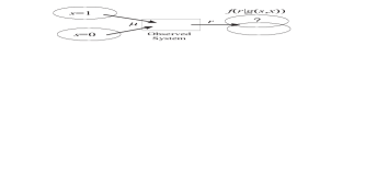
Figure 1: General set separation system

The general set separation system is depicted in Fig. 1. The observed signal $r$, disturbed by the system $A$, becomes the input data which will be separated into the two sets ($s=0$ and $s=1$) again.

In the set separator a quantum register $|\varphi\rangle$ –as described by equation (1) and shown in Fig. 2.– is used to store all the parameters, e.g. delay, heat, velocity, etc. values of the possible system disturbance in a specially given quantization. As an example: in the qregister $|\varphi\rangle$, the properly prepared, quantized delay and velocity values are stored, e.g. the values $1.0\cdot 10^{-1},1.1\cdot 10^{-1},\ldots,1.0\cdot 10^{-10}$ and $1.0~{}m/s,1.1~{}m/s,\ldots,100~{}m/s$. This information is not utilizable so far but the combination of this effects, i.e. this values, whose extent could blast any database. To handle the large amount of data to be processed a virtual database should be introduced.

Definition 3.1

To build up a virtual database a function

$$y=g(s,\underline{x}),$$ (2)

is defined, where $s\in S$ identifies the sets and $\underline{x}$ denotes the index of the qregister $|\varphi\rangle$, respectively. The function $y_{i}=g(s,x_{i})$ points to an record in the virtual database.

3.1 Properties of the Function $g(\cdot)$

The function $g(s,\underline{x})$ is not obligingly mutual unambiguous consequently, it is not reversible, except for several special cases, when the virtual database contains $\widehat{r}=g(s,\underline{x})$ only once. In this case the parameter settings of the system $A$ are easy to determine. Nevertheless, the fact to have an entry only once in the virtual database described by the equation $g(s_{i},\underline{x})$ does not exclude to have the same entry in other virtual databases generated by $g(s_{j},\underline{x})$, where $i\neq j$, which makes a trivial decision impossible. Henceforth the fact should be kept in mind that $g(s,\underline{x})$ is in almost every case a so called one way function which is easy to evaluate in one direction, but to estimate the inverse is rather hard.

The function $g(.)$ generates all the possible disturbances additional to the considered input value $\mu$ belonging to the set $s=0$ or $s=1$ of the system. This is of course a large amount of information, $2N=2^{n+1}$, where $n$ is the length of the qregister $|\varphi\rangle$. For an example let us assume a 15-qbit qregister. The function $g(\cdot)$ in (2) generates $2^{15}=32.768$ output values at the same time for $s=0$ and the same number of outputs for $s=1$. Taking into account the large number of possible points in the set surface the optimal classification in a classical way becomes difficult.

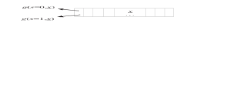
Figure 2: Quantum register $|\varphi\rangle$

At the first glace this problem looks more difficult to solve, however, with exploiting the enormous computational power of quantum computation, in this case the Deutsch-Jozsa [7] quantum parallelization algorithm, an arbitrary unitary operation can be executed on all the prepared states contemporaneously.

3.2 Quantum Search in Qregister $|\varphi\rangle$

Roughly speaking the task is to find the entry (entries) in the virtual databases which is (are) equal to the observed data $r$. To accomplish the database search the Grover database search algorithm should be invoked [8]. In Sect. 2. we proposed to set up an qregister, which has to be built up only one time at all. It is obvious to choose a suitable database searching algorithm, to see which function $g_{0,1}(s_{0,1},\underline{x})$ picking the vector $\underline{x}$ form qregister $|\varphi\rangle$ contains the searched bit, if any at all. We apply the optimal quantum search algorithm $\mathcal{G}$, as depicted in Fig. 3. proposed by Grover [9, 10]. We feed the received signal $r(t)$ to the oracle $(\mathrm{O})$, where the function $f(r,g(s,\underline{x})$$)$ is evaluated such that

$$f(a,b)=\left\{\begin{array}[]{cl}\mbox{1}&\mbox{if $a=b$}\\ 0&\mbox{otherwise}.\end{array}\right.$$ (3)

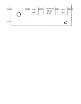
Figure 3: The Grover database search circuit

Assuming, there is again $M$ solutions for the search in qregister $|\varphi\rangle$,

$$\mbox{$|\varphi\rangle$}=\sqrt{\frac{N_{s}-M}{N_{s}}}\mbox{$|\alpha\rangle$}+\sqrt{\frac{M}{N_{s}}}\mbox{$|\beta\rangle$},$$ (4)

where $|\alpha\rangle$ consists of such configurations of $|x\rangle$, which does not results $\widehat{\mu}=r$, while $|\beta\rangle$ does.

Because of the fact of tight bound, in real application less iterations would be also appropriate [11].

4 Set Separation

Let us turn our interest back to the separation of the observed data $r$ from the predefined sets.

Assuming the special case where only one of the virtual database descriptor functions, either $g(s_{0},\underline{x})$ or $g(s_{1},\underline{x})$ contains the entry identical to the observed data $r$ a set separation can be performed easily.

A more realistic case is to have an intersection part of the two sets as shown in Fig. 4. Even so, due to passing the observed system, overlapping of the sets can be occurred due to disturbances. After evaluating the functions $g_{0,1}(s_{0,1},\underline{x})$ it could happen that the same records are multiple present, which shows the irreversibility behavior of the function (2). Originally, the input signal was chosen from well defined disjunct sets without a-priori known probability distributions. The process, to put $r$ to a set either to $s_{0}$ or to $s_{1}$ should be based on Maximum Likelihood decision.

Let us assume that we have a random variable $r$. Its measured value depends on a selected element $x_{l}$ from a finite set ($l=1,\ldots,L$) and a process which can be characterized by means of a conditional pdf $f(r|x_{l})$ belonging to the given element. Our task is to decide which $x_{l}$ was selected if a certain $r$ has been measured. Each guess $H_{l}$ for $x_{l}$ can be regarded as a hypothesis. Therefore decision theory is dealing with design and analysis of suitable rules building connections between the set of observations and hypotheses.

If we are familiar with the unconditional (a priori) probabilities $P(x_{l})$ then the Bayes formula helps us to compute the conditional (a posteriori) probabilities $P(H_{i}|r)$ in the following way

$$P(H_{l}|r)=\frac{f(r|x_{l})P(x_{l})}{\sum^{L}_{i=1}f(r|x_{i})P(x_{i})}.$$

Obviously the most pragmatic solution if one chooses $H_{l}$ belonging to the largest $P(H_{l}|r)$. This type of hypothesis testing is called maximum a posteriori (MAP) decision.

If the a priori probabilities are unknown or $x_{l}$ is equiprobable then maximum likelihood (ML) decision can be used. It selects $H_{l}$ resulting the largest $f(r|x_{l})$ when the observed $r$ is substituted in order to minimize the probability of error

Figure 4: Sets with intersection

$$\max_{l}L(r,x_{l}).$$

The Maximum Likelihood estimator requires to know the probability density function of the observed signal. Employing the Grover database search algorithm we are able to find the entries in the virtual databases, however, it is not needed to perform a complete search because the search result –the exact index (indices) of the searched item(s)– is (are) not interesting but the number how often a given configuration is involved in $g(s,\underline{x})$ or not. For that purpose a new function $f(\cdot)$ is defined.

Definition 4.1

The function

$$f(r|s)=\frac{\sharp\left(x:r=g(s,x)\right)}{\sharp(x)},$$ (5)

counts the number of similar entries in the virtual database, which corresponds to the conditional probability density function $r$ to be in the set $s$.

For that reason it is worth stepping forward to quantum counting [12] based on Grover iteration.

4.1 Set Separation Method

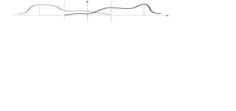
Figure 5: The two density functions $f\left(r|s=0\right)$ and $f\left(r|s=1\right)$

The both curves in Fig. 5. represent the number of the same entries in the virtual databases, i.e. the pdf’s, according to $f(r|s=0)$ and $f(r|s=1)$, respectively. In case of having entry(entries) only in $y_{i}$ but not in $y_{j}$ of function $g_{0,1}(s_{0,1},\underline{x})$, where $i,j\in[0,1]$, and $i\neq j$, means a 100 percent sure decision, following the decision rules in Table 1. This areas are the non-overlapping parts of the sets in Fig. 4. and the outer parts (until the vertical dashed black lines) in Fig. 5. However, in the case of non zero $f(r|s=0)$ and $f(r|s=1)$ values an accurate prediction can be given relating to the Maximum Likelihood decision rule.

Table 1: Set Separation Decision Rules

$f(r|s_{0})$	$f(r|s_{1})$	Decision
0	0	$|\varphi\rangle$ was badly prepared
0	$\neq 0$	$r$ belongs to set $s=1$
$\neq 0$	0	$r$ belongs to set $s=0$
$>$		$r$ belongs to set $s=0$
$<$		$r$ belongs to set $s=1$

All the possible states from the qregister $|\varphi\rangle$ will be evaluated by the function (2) for $s=0$ and also for $s=1$, simultaneously, which will be collated with the system output $r$. If at least one output $y_{0}$ or $y_{1}$ with the parameter settings $x$ is matched to the system output $r$, it will be put to the set $s=0$ or $s=1$, respectively. In a more exciting case at least one similarity of $y_{0}$ and also at least one of $y_{1}$ to $r$ is given, the system output could be classified to the both sets, an intersection is drawn up. This result in a not certainty prediction, which piques our interest and sets our focus not this juncture.

We assume no a-priori knowledge on the probability distribution of the input sequence $\mu$, so it is assumed to be equally distributed. Henceforward we suppose that after counting the evaluated values $f(r|s=i)$ the number of similarity to the system output $r$ is higher than in case of $f(r|s=j)$, where $i,j\in[0,1]$. In pursuance of the decision rule in Table 1., $r$ belongs rather to set $s=i$ than to set $s=j$.

The Method

To perform a set separation nothing else is required as

1. Prepare the qregister $|\varphi\rangle$,

2. Evaluate the functions $y_{i}=g_{i}=(s=i,\underline{x})$, where $i\in[0,1]$ in 2-dimensional case,

3. Count the identical entries in the virtual databases which are equal to the observed data $r$, $f(r|s)$, (see Fig. 5).,

4. Use the decision table Table 1 to assign $r$ to the sets $s=0$ or $s=1$.

5 Concluding Remarks

In this paper we showed a connection between Maximum Likelihood hypothesis testing and Quantum Counting used for quantum set separation. We introduced a set separation algorithm based on quantum counting which was employed to estimate the conditional probability density function of the observed data in consideration to the belonging sets. In our case the pdf’s are estimated fully at a single point by invoking the quantum counting operation only once, that makes the decision facile and sure. In addition one should keep in mind that the qregister $|\varphi\rangle$ have to be set up only once before the separation. The virtual databases are generated once and directly leaded to the Oracle of the Grover block in the quantum counting circuite, which reduce the computational complexity, substantially.

References

- [1] K. Fukunaga, Introduction to Statistical Pattern Recognition, 2nd ed., ser. Electrical Science, H.G. Booker & N. DeClaris, Ed. New York, London: Academia Press, INC., 1972.
- [2] P. Shor, “Quantum computing,” Documenta Mathematica, vol. 1-1000, 1998, extra Volume ICM.
- [3] D. Deutsch, “Quantum theory of probability and decisions,” Proc. R. Soc. London, Ser. A, 2000.
- [4] M.A. Nielsen, I.L. Chuang, Quantum Computation and Quantum Information. Cambridge University Press, 2000.
- [5] A. Ekert, P. Hayden, H. Inamori, “Basic concepts in quantum computation,” 16 January 2000.
- [6] S. Imre, F. Balázs, “Quantum multi-user detection,” Proc. 1st. Workshop on Wireless Services & Applications, Paris-Evry, France, pp. 147–154, July 2001, iSBN: 2-7462-0305-7.
- [7] D. Deutsch, R. Jozsa, “Rapid solution of problems by quantum computation,” Proc. R. Soc. London, Ser. A, pp. 439,553, 1992.
- [8] L. Grover, “A fast quantum mechanical algorithm for database search,” Proceedings, 28th Annual ACM Symposium on the Theory of Computing, pp. 212–219, May 1996, e-print quant-ph/9605043.
- [9] ——, “How fast can a quantum computer search?” April 1999.
- [10] C. Zalka, “Grover’s quantum searching algorithm is optimal, e-print quant-ph/9711070v2,” December 1999.
- [11] S. Imre, F. Balázs, “The generalized quantum database search algorithm,” Submitted to Computing, 2003.
- [12] G. Brassard, P. Hoyer, A. Tapp, “Quantum counting,” Lecture Notes in Computer Science, vol. 1443, pp. 820+, 1998. [Online]. Available: http://xxx.lanl.gov/archives/9805082