Two qubits entanglement dynamics in a symmetry-broken environment

Abstract

We study the temporal evolution of entanglement pertaining to two qubits interacting with a thermal bath. In particular we consider the simplest nontrivial spin bath models where symmetry breaking occurs and treat them by mean field approximation. We analytically find decoherence free entangled states as well as entangled states with an exponential decay of the quantum correlation at finite temperature.

I Introduction

Since 1935 sch ; epr , entanglement has been recognized as one of the most puzzling features of Quantum Mechanics. However, it is nowadays a widespread opinion that it also represents a fundamental resource for many quantum information protocols. As such, entanglement deserves to be analyzed in all respects. A primary concern is its robustness against environmental effects, and a supplied literature exists aimed at preserving entanglement coherence vio1 ; vio2 ; vio3 ; vio4 ; vio5 ; vio6 ; vio7 . More recently, attention has been devoted to the problem of thermal entanglement gun i.e. quantifying entanglement arising in spin chains at thermal equilibrium with a bath. In this approach environment determines the temperature $T$ to allow for a thermal distribution of system energy levels, while the detailed interaction between system and environment is not an essential part of the matter. The same is true also for those works that focus on entanglement decoherence yu ; yu2 (also known as disentanglement ter ; bla ). In this context the study of entanglement time behaviour is carried on with a master equation formalism and markovian approximation gar or, more generally, with arguments provided by spin-boson models.

In the present paper we are going to envisage a novel approach to the problem along the line introduced for the first time in Ref.dep (a similar outline but supported by numerical means is also present in tess ). There, the authors considered a one spin system interacting with a fermionic environment endowed with a structure capable of symmetry-breaking sac . It was shown by analytical methods that coherence time increases as magnetic order enlarges or, in other terms, as temperature decreases. Here we extend this argument to a two qubits system plunged in a fermionic environment described by Transverse Ising model (TIM) and Ising model (IM) sac . We shall examine the time evolution of concurrence of the bipartite system woo , and find environment-limited concurrences as well as unlimited ones according to environment ordering level.

The paper is organized as follows: in section II we introduce the model by referring to dep and we revise some results. In section III we extend the model to a bipartite systems, and we present the results of paradigmatic cases in Sec. IV. Finally, Sec. V is for conclusions. Explicit calculations are reported in Appendices A and B.

II The Model

We consider the general scenario of a system and a bath described by hamiltonians $H_{s}$ and $H_{B}$ respectively, and interacting through the hamiltonian $H_{sB}$. The total hamiltonian is then $H=H_{s}+H_{sB}+H_{B}$, and the initial density matrix is assumed to be factorized, i.e., $\rho(0)=\rho_{s}\otimes\rho_{B}$. We are looking for the time evolution of the reduced system density matrix $\rho_{s}(t)$; in particular we are interested in its off diagonal elements, the so called “coherences”. If $H$ doesn’t depend on time the total density matrix will evolve accordingly to

$$\rho\left(t\right)=e^{-iHt}\rho(0)e^{iHt}\,.$$ (1)

We can then obtain the reduced density matrix by tracing out the bath degrees of freedom in Eq.(1)

$$\rho_{s}\left(t\right)=tr_{B}\rho(t)\,.$$ (2)

We now follow the line sketched in Ref.dep to introduce the model for a spin system interacting with a spin bath. First of all, we assume the bath density matrix having a thermal distribution, that is $\rho_{B}=(e^{-H_{B}/T})/Z$, with $T$ the bath temperature multiplied by the Boltzmann constant, and $Z=tr\left(e^{-H_{B}/T}\right)$ the partition function. Furthermore, we ask the bath hamiltonian to be a “symmetry breakable” one, that is endowed with phase transition in the degrees of freedom that provide the coupling with the system. The simplest hamiltonian with these requirements is a long ranged Ising Model-like one (IM). We add to it a transverse field to include a more general case in the analysis, dealing eventually with a Transverse Ising Model bath hamiltonian (TIM). The differences between the two models are minimal as coherence and entanglement is concerning and, in any case, we will be able to find results for IM in the limit of no transverse field for TIM. These peculiar environment hamiltonians will be studied through mean field approximation sac .

II.1 TIM-environment

Let us consider $N+1$ spin-$\frac{1}{2}$, and let $S_{j}^{\alpha}$ be the $\alpha$ component ($\alpha=x,\,y,\,z$) of the $j$th spin ($j=0,1,\ldots,N$). The label $j=0$ refers to the system operators while $j=1,\ldots,N$ to the bath operators. Furthermore, $S_{j}^{\pm}=(S_{j}^{x}\pm iS_{j}^{y})/2$ are the spin flip operators, and $|0\rangle$ and $|1\rangle$ are the lower and upper eigenstates of $S^{z}$. The following hamiltonians define the energy of the system, of the TIM-bath and of the interaction between them:

$$H_{s} = -\mu_{0}\,S_{0}^{z},$$ (3a)

$$H_{sB} = -\frac{J_{0}}{\sqrt{N}}S_{0}^{z}\sum\limits_{k}S_{k}^{z}\,,$$ (3b)

$$H_{B} = -w\sum\limits_{k}S_{k}^{x}-\frac{J}{N}\sum\limits_{i,k}S_{i}^{z}S_{k}^{z}\,,$$ (3c)

where $\mu_{0}$ is the coupling constant with an external magnetic field parallel to the $\hat{z}$ axis, $J_{0}$, $J$ are exchange coupling constants and $w$ is the strength of the transverse field; they are all non negative constants. The indices of the sums run from $1$ to $N$. Eq.(3c) describes a material in which spins compete to align along the positive direction of $\hat{x}$ axis or along $\hat{z}$ axis following a ferromagnetic behaviour; of course in the latter case the absolute direction of alignment is not important since the hamiltonian is symmetric in $z$-operators. We can notice that energy exchanges between system and bath are not included in the interaction hamiltonian; this will generate a pure dephasing dynamics, in which energy will be conserved, and temporal evolution analytically solved.

The main difficulty with Eqs.(3) is represented by the nonlinear term in $H_{B}$. For this reason it is helpful to approximate it with a mean field bath hamiltonian, as explained in dep :

$$H_{B}^{mf}=-w\sum\limits_{k}S_{k}^{x}-2Jm\sum\limits_{k}S_{k}^{z}+m^{2}JN\,.$$ (4)

In the above equation $m$ is the order parameter of the phase transition. Its absolute value ranges from $0$ to $\frac{1}{2}$ as long as temperature ranges from the critical value $T_{c}=\frac{J}{2}$ to $0$ : the greater $|m|$ the larger the magnetic order of the bath along $\hat{z}$ axis. In the following we are going to consider only positive values for $m$ since results are sign-independent. Everything remains true with the substitution $m\rightarrow-m$. This is a consequence of $H_{B}$ $z$-symmetry, that is not lost in $H_{B}^{mf}$. The order parameter $m$ is implicitly defined by the following self-consistent equation for the quantity $\Theta=\pm\sqrt{w^{2}+4m^{2}J^{2}}$ (also $\Theta$’s sign, written here for sake of precision, is irrelevant, for the same reasons of $m$’s):

$$\frac{\Theta}{J}=\tanh\frac{\Theta}{2T}.\,$$ (5)

It is worth noting that from Eq.(5) we have $\Theta\rightarrow J$ for $T\rightarrow 0$; furthermore, from the definition of $\Theta$, we can see it tends to $2mJ$ in the limit of no transverse field ($w\rightarrow 0$).

Together with Eq.(5) we must consider the following condition on the transverse field to obtain an ordered phase with TIM:

$$\frac{w}{J}<\tanh\left(\frac{w}{2T}\right).$$ (6)

This condition is not satisfied in the range of temperatures above $T_{c}$; for this reason the whole formalism we are using is valid only in the broken phase.

With the linearized mean field bath hamiltonian it is possible to evaluate the coherence of the system (see Appendix A):

$$S_{0}^{-}(t) = tr_{B}\left[e^{-iH^{mf}t}\left(S_{0}^{-}(0)\otimes\rho_{B}\right)e^{iH^{mf}t}\right]$$ (7)

$$= \frac{1}{Z}tr_{B}\left[e^{-iH^{mf}t}\left(\left|0\right\rangle\left\langle 1\right|\otimes e^{-H_{B}^{mf}/T}\right)e^{iH^{mf}t}\right]$$

$$= S_{0}^{-}(0)r_{{}_{TIM}}(t)$$

where $H^{mf}=H_{s}+H_{sB}+H^{mf}_{B}$, and

$$r_{{}_{TIM}}(t)=\left[\cos\left(\frac{tmJJ_{0}}{\Theta\sqrt{N}}\right)+i\frac{\Theta}{J}\sin\left(\frac{tmJJ_{0}}{\Theta\sqrt{N}}\right)\right].$$ (8)

Equation (7) tells us that the time evolution of the off diagonal term of the system density matrix, responsible for the coherence of the system, is enclosed in the time behaviour of the complex valued factor $r_{{}_{TIM}}(t)$. In particular, in order to find system decoherence, we ask whether and when this factor’s absolute value goes to zero. In the limit of large $N$ we can approximate it as:

$$\left|r_{{}_{TIM}}(t)\right|\approx\exp\left[{-\frac{J_{0}^{2}m^{2}t^{2}}{2}\left(\frac{J^{2}}{\Theta^{2}}-1\right)}\right]\,.$$ (9)

We can see from (9) that the system coherence decays exponentially with time. The coherence time is:

$$\tau_{{}_{TIM}}=\frac{\left|\Theta\right|}{J_{0}m}\sqrt{\frac{2}{J^{2}-\Theta^{2}}}\,,$$ (10)

and increases as temperature decreases; for $T=0$ it is $\tau=\infty$, and the system remains coherent. This is quite a counter-intuitive effect since collective quantum properties of materials endowed with phase transition disappear as ordering increases (see for instance Ref. jon ). The factor $t^{2}$ in the exponent denotes the intrinsically reversible nature of the process, in contrast to irreversibility introduced by markovian approach, and is closely related to the “Zeno effect” zur . In particular the periodicity of $r_{{}_{TIM}}(t)$ in Eq.(8) leads to the so called “recoherences” on a Poincaré time scale. Decoherence takes place in the limit of an environment with infinite degrees of freedom; besides, the same limit is necessary to support the mean field theory approach we adopted. Thus in this context the limit $N\rightarrow\infty$ has a double function: to take into account the decoherence process and to give a meaning to the mean field approximation written above.

We briefly notice here that the factor $r_{{}_{TIM}}(t)$ in Eq.(9) is exactly alike to $r_{as}(t)$ of Eq.(32) in dep . But as far as that paper is concerning we must point out some inaccuracies: the final result (32) is correct, but the intermediate steps to find it are not. In particular the general formula (11) applies only if the $3\times 3$ matrices $\Lambda_{k}$ commute, and this is not true when you look at Eq.(29) of that article. For this reason the intermediate formula (30) is wrong and the oscillations showed in Fig.1 are not present.

II.2 Limit of no transverse field: IM-environment

In the limit of $w\rightarrow 0$ we obtain from (3) the IM-hamiltonians which lead to

$$\left|r_{{}_{IM}}(t)\right|\approx\exp\left[-\frac{J_{0}^{2}t^{2}}{2}\left(\frac{1}{4}-m^{2}\right)\right]\,.$$ (11)

We can notice the same behaviour as for TIM-bath, but slightly more transparent: the coherence time is $\tau_{{}_{IM}}=\frac{2}{J_{0}}\sqrt{\frac{2}{1-4m^{2}}}$ and its limits are $\tau_{{}_{IM}}^{(T=T_{c})}=\frac{2\sqrt{2}}{J_{0}}$ and $\tau_{{}_{IM}}^{(T=0)}=\infty$. We note that coherence explicit dependence on bath coupling constant $J$ has disappeared in this case; only interaction coupling constant $J_{0}$ enters coherence expression when the bath is an IM-one. Otherwise the $J$ coupling is indirectly present in (11) because it has a role in determining the order parameter $m$ by means of Eq.(5).

III The Extension

In this section we extend results obtained in the previous one by considering a two qubits system, and studying the time evolution of their entanglement. We assume that the system qubits, labeled by $01$ and $02$, interact between them and with environment, that is symmetry-breakable and modeled by TIM hamiltonians generalizing those of Eqs.(3):

$$H_{s} = -\xi_{0}S_{01}^{z}S_{02}^{z},$$ (12a)

$$H_{sB} = -\frac{J_{0}}{\sqrt{N}}\left(S_{01}^{z}+S_{02}^{z}\right)\sum\limits_{k}S_{k}^{z}\,,$$ (12b)

$$H_{B} = -w\sum\limits_{k}S_{k}^{x}-\frac{J}{N}\sum\limits_{i,k}S_{i}^{z}S_{k}^{z}\,,$$ (12c)

In above equations $\xi_{0}$ represents the coupling constant between the qubits. We have discarded both local interactions, like that between qubits and an external magnetic field, and local couplings with environment degrees of freedom, a situation resembling a “collective” system-environment pairing vio5 .

As a measure of entanglement between two qubits we adopt the so called “concurrence” woo , which ranges from $0$ for separable states to $1$ for maximally entangled states. The concurrence is given by:

$$C=\max\left\{\lambda_{1}-\lambda_{2}-\lambda_{3}-\lambda_{4},0\right\}\text{,}$$ (13)

where $\lambda_{1}$, $\lambda_{2}$, $\lambda_{3}$ and $\lambda_{4}$ are the square roots of the eigenvalues, in decreasing order, of the matrix $R=\rho_{s}\widetilde{\rho_{s}}$. Here $\rho_{s}$ is the density matrix of the 2 system qubits, and $\widetilde{\rho_{s}}$ is the “time reversed” matrix given by

$$\widetilde{\rho_{s}}=\left(\sigma^{y}_{01}\otimes\sigma^{y}_{02}\right)\rho_{s}^{\ast}\left(\sigma^{y}_{01}\otimes\sigma^{y}_{02}\right)\,,$$ (14)

where $\sigma$’s are the usual Pauli matrices. The symbol $\rho_{s}^{\ast}$ means complex conjugation of the matrix $\rho_{s}$ in the standard basis $\left|00\right\rangle$, $\left|01\right\rangle$, $\left|10\right\rangle$, $\left|11\right\rangle$.

We assume that the qubits are initially decoupled from the environment, and the bath having a thermal density matrix $\rho_{B}=(e^{-H_{B}/T})/Z$. Therefore, we can write the whole state as:

$$\rho=\left|\Psi\right\rangle\left\langle\Psi\right|\otimes\rho_{B}$$ (15)

with a generic system pure state:

$$\left|\Psi\right\rangle=\alpha\left|00\right\rangle+\beta\left|01\right\rangle+\gamma\left|10\right\rangle+\delta\left|11\right\rangle\,,\qquad|\alpha|^{2}+|\beta|^{2}+|\gamma|^{2}+|\delta|^{2}=1\,.$$ (16)

The steps to find time evolution of Eq.(15) are similar to those leading to Eq.(7) (see Appendix A), but now operators are represented by $4\times 4$ matrices, being our system composed by two qubits. After mean field approximation (4) for the bath hamiltonian and some elementary algebra we obtain the reduced density matrix as:

$$\rho_{s}\left(t\right)=tr_{B}\left(\rho\left(t\right)\right)=\left(\begin{array}[]{cccc}\left|\alpha\right|^{2}&\alpha^{\ast}\beta A^{\ast}e^{-\frac{1}{2}it\xi_{0}}&\alpha^{\ast}\gamma A^{\ast}e^{-\frac{1}{2}it\xi_{0}}&\alpha^{\ast}\delta B^{\ast}\\ \alpha\beta^{\ast}Ae^{\frac{1}{2}it\xi_{0}}&\left|\beta\right|^{2}&\beta^{\ast}\gamma&\beta^{\ast}\delta A^{\ast}e^{\frac{1}{2}it\xi_{0}}\\ \alpha\gamma^{\ast}Ae^{\frac{1}{2}it\xi_{0}}&\beta\gamma^{\ast}&\left|\gamma\right|^{2}&\gamma^{\ast}\delta A^{\ast}e^{\frac{1}{2}it\xi_{0}}\\ \alpha\delta^{\ast}B&\beta\delta^{\ast}Ae^{-\frac{1}{2}it\xi_{0}}&\gamma\delta^{\ast}Ae^{-\frac{1}{2}it\xi_{0}}&\left|\delta\right|^{2}\end{array}\right)\,,$$ (17)

where the coefficients

$$A = \left[\cos\left(\frac{tmJJ_{0}}{\Theta\sqrt{N}}\right)+i\frac{\Theta}{J}\sin\left(\frac{tmJJ_{0}}{\Theta\sqrt{N}}\right)\right]^{N}\,,$$ (18a)

$$B = \left[\cos\left(\frac{2tmJJ_{0}}{\Theta\sqrt{N}}\right)+i\frac{\Theta}{J}\sin\left(\frac{2tmJJ_{0}}{\Theta\sqrt{N}}\right)\right]^{N}\,,$$ (18b)

characterize the time dependence of the concurrence. From the above expression of $\rho_{s}(t)$ we can find the matrix $R(t)$ and its eigenvalues, and from them, as explained, the final concurrence of the system. The complete expression for $R(t)$ and for coefficients of Eq.(18) is given in Appendix B. In the following we are going to consider some paradigmatic cases for the initial state (15).

IV Paradigmatic cases

IV.0.1 Case 1

Let us set $\alpha=\delta=0$ in Eq.(16) for the initial state of the system. We obtain $\left|\Psi\right\rangle=\beta\left|01\right\rangle+\gamma\left|10\right\rangle$ and $R$ matrix reduces to:

$$R(t)=\left(\begin{array}[]{cccc}0&0&0&0\\ 0&2\left|\beta\right|^{2}\left|\gamma\right|^{2}&2\beta^{\ast}\left|\beta\right|^{2}\gamma&0\\ 0&2\beta\gamma^{\ast}\left|\gamma\right|^{2}&2\left|\beta\right|^{2}\left|\gamma\right|^{2}&0\\ 0&0&0&0\end{array}\right)\,,$$ (19)

whose square rooted eigenvalues are:

$$\lambda_{1} = 2\left|\beta\right|\left|\gamma\right|\,,$$ (20a)

$$\lambda_{2} = \lambda_{3}=\lambda_{4}=0\,,$$ (20b)

This leads to the following concurrence:

$$C_{{}_{TIM}}=2\left|\beta\right|\left|\gamma\right|\,.$$ (21)

The entanglement results time independent, so the state does not perceive the presence of the environment. The reason is that $|\Psi\rangle$ is an eigenstate of the interaction hamiltonian and so it represents a decoherence free entangled state vio5 . Since $w$ is not present in the concurrence written above we know that the expression for the concurrence would be exactly the same for an IM-environment.

IV.0.2 Case 2

Now we set $\beta=\gamma=0$ in Eq.(16) and obtain the state $\left|\Psi\right\rangle=\alpha\left|00\right\rangle+\delta\left|11\right\rangle$. The $R$ matrix becomes:

$$R(t)=\left(\begin{array}[]{cccc}\left|\alpha\right|^{2}\left|\delta\right|^{2}\left(1+\left|B\right|^{2}\right)&0&0&2\alpha^{\ast}\left|\alpha\right|^{2}\delta B^{\ast}\\ 0&0&0&0\\ 0&0&0&0\\ 2\alpha\delta^{\ast}\left|\delta\right|^{2}B&0&0&\left|\alpha\right|^{2}\left|\delta\right|^{2}\left(1+\left|B\right|^{2}\right)\end{array}\right)\,,$$ (22)

with square rooted eigenvalues in decreasing order:

$$\lambda_{1} = \left|\alpha\right|\left|\delta\right|\left(\left|B\right|+1\right)\,,$$ (23a)

$$\lambda_{2} = \left|\alpha\right|\left|\delta\right|\left(\left|\left|B\right|-1\right|\right)\,,$$ (23b)

$$\lambda_{3} = \lambda_{4}=0\,.$$ (23c)

¿From Eqs.(18), for large $N$, we get:

$$\left|B\right|\approx\exp\left[-2J_{0}^{2}m^{2}t^{2}\left(\frac{J^{2}}{\Theta^{2}}-1\right)\right].\$$ (24)

Then, by using concurrence definition and Eqs.(23), we arrive at:

$$C_{{}_{TIM}}=2\left|\alpha\right|\left|\delta\right|\left|B\right|=2\left|\alpha\right|\left|\delta\right|\exp\left[-2J_{0}^{2}m^{2}t^{2}\left(\frac{J^{2}}{\Theta^{2}}-1\right)\right].\$$ (25)

Figure 1: Concurrence versus scaled time $J_{0}t$. Curves from the left to the right are for $\frac{T}{T_{c}}=\{.75,.50,.35,.25\}$. The value of other parameter are $w=0.1,J=2$.

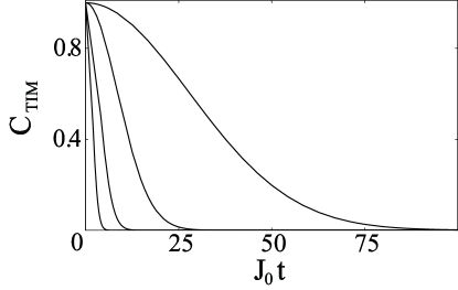
The time behaviour of the concurrence just obtained is shown in Fig.1 for different values of the ratio $\frac{T}{T_{c}}$. We notice that in this case the qubits perceive the presence of the thermal bath, which spoils entanglement between them; in fact the initial state is no longer an eigenstate of the interaction hamiltonian. Only for zero temperature the order parameter reaches its saturation value and the concurrence remains constant. The behaviour is very similar to that of one qubit system coherence described by Eq.(7), but entanglement decoherence is exactly twice faster than one qubit decoherence. This result agrees with what found in yu2 . Furthermore, together with the previous case, it falls within the general limitations represented by the Universal Disentangling Machine ter .

In the limit $w\rightarrow 0$ we obtain the concurrence for an IM-bath:

$$C_{{}_{IM}}=2\left|\alpha\right|\left|\delta\right|\exp\left[-2J_{0}^{2}t^{2}\left(\frac{1}{4}-m^{2}\right)\right]\,.$$ (26)

Analogously to what already noticed for the single qubit coherence, in this limit the factor $J$ disappears from the explicit concurrence expression. The only exchange coupling constant that enters in the decoherence time for the concurrence is $J_{0}$.

IV.0.3 Case 3

If we set $\alpha=\beta=0$ we obtain a product state $\left|\Psi\right\rangle=\gamma\left|10\right\rangle+\delta\left|11\right\rangle=\left(\gamma\left|0\right\rangle+\delta\left|1\right\rangle\right)\left|1\right\rangle$, which trivially gives:

$$R(t)=\left(\mathbf{0}\right)\Longrightarrow C=0\,.$$ (27)

In this case TIM hamiltonians are not able to induce entanglement between system qubits.

IV.0.4 Case 4

If we set $\alpha=\beta=\gamma=\delta=\frac{1}{2}$ we obtain again a separable initial state, but different from the previous one: $\left|\Psi\right\rangle=\frac{1}{2}\left(\left|00\right\rangle+\left|01\right\rangle+\left|10\right\rangle+\left|11\right\rangle\right)=\frac{1}{\sqrt{2}}\left(\left|0\right\rangle+\left|1\right\rangle\right)\frac{1}{\sqrt{2}}\left(\left|0\right\rangle+\left|1\right\rangle\right)$. In this case the $R$ matrix is not trivial:

$$R(t)=\frac{1}{16}\left(\begin{array}[]{cccc}1+\left|B\right|^{2}-2\left|A\right|^{2}e^{-it\xi_{0}}&U_{\xi_{0}}&U_{\xi_{0}}&2B^{\ast}-2\left(A^{\ast}\right)^{2}e^{-it\xi_{0}}\\ -V_{\xi_{0}}&2-2\left|A\right|^{2}e^{it\xi_{0}}&2-2\left|A\right|^{2}e^{it\xi_{0}}&-U_{\xi_{0}}\\ -V_{\xi_{0}}&2-2\left|A\right|^{2}e^{it\xi_{0}}&2-2\left|A\right|^{2}e^{it\xi_{0}}&-U_{\xi_{0}}\\ 2B-2A^{2}e^{-it\xi_{0}}&V_{\xi_{0}}&V_{\xi_{0}}&1+\left|B\right|^{2}-2\left|A\right|^{2}e^{-it\xi_{0}}\end{array}\allowbreak\right)\,,$$ (28)

where:

$$U_{\xi_{0}} = \left(2A^{\ast}e^{-\frac{1}{2}it\xi_{0}}-\left(A^{\ast}+AB^{\ast}\right)e^{\frac{1}{2}it\xi_{0}}\right)$$ (29a)

$$V_{\xi_{0}} = \left(2Ae^{-\frac{1}{2}it\xi_{0}}-\left(A+A^{\ast}B\right)e^{\frac{1}{2}it\xi_{0}}\right)$$ (29b)

The concurrence is evaluable esplicitly, but the expression is too much cumbersome therefore not reported here. We only show in Fig.2 its behaviour.

Figure 2: Concurrence versus the scaled time $J_{0}t$. The plot shows the limiting role of decoherence (dotted line) that falls down exponentially, on entanglement (continuous line). The value of parameters are $w=0.1,\xi_{0}=0.3,J=2,\frac{T}{T_{c}}=.25$.

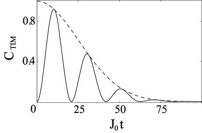
The concurrence starts from its null value and increases because of the interaction between system qubits. If there wasn’t disentanglement it would reach its maximum and decrease again giving rise to oscillations of equal amplitude. Nevertheless, the presence of environment alters this temporal behaviour damping the oscillations. For suitable values of coupling constants it can even prevent qubits from entangling at all. The interesting question of the maximal entanglement generation under dephasing processes arises naturally in this case yu .

V Conclusion

We have studied time behaviour of entanglement between two qubits dipped in a large symmetry-breakable fermionic environment, below the critical temperature $T_{c}$. In the frame of mean field theory analytical results are provided for concurrence of the bipartite system, with temperature as a parameter of the problem. The hamiltonians involved in the discussion are those typical of Transverse Ising Models (TIM), capable of magnetic ordering under suitable conditions. To assign them a physical meaning we notice that, upon addition of a transverse field in $H_{s}$, our model resembles an array of Rydberg atoms interacting with a cavity mode of the radiation field dep . Nevertheless such an assumption for $H_{s}$ makes the problem unsolvable by analytical techniques, and requires numerical investigation that we plan to accomplish in a near future. Beside that an important improvement would be to overcome mean field approximations adopted in the text, by including the effect of fluctuations, or by applying the spin wave approach spa to the bath.

What comes out from the paper is quite a counterintuitive conservation of entanglement in a bath with strong interactions: the bigger the coupling strength (or the lower the ratio $\frac{T}{T_{c}}$) the longer the time qubits remain entangled (Eq.(25) and Fig.(1)). In some cases entangled qubits don’t perceive environment at all, and the system state is a decoherence free one (Eq.(21)). Several connections with results from the field of entanglement decoherence are provided. We believe our analysis can be useful to complete knowledge about entanglement dynamical properties.

Appendix A

A.1 Exponentiation of suitable matrices

Let us define a $2\times 2$ traceless matrix ${\cal A}$ as

$${\cal A}=\left(a\sigma_{x}+b\sigma_{z}\right)=\left(\begin{array}[]{cc}b&a\\ a&-b\end{array}\right)\,,$$ (30)

with $a$, $b$ real coefficients. The exponentiation of $A$ gives:

$$e^{\cal A}=\left(\cosh q\right)I+\left(\frac{\sinh q}{q}\right){\cal A}\,;e^{i\cal A}=\left(\cos q\right)I+i\left(\frac{\sin q}{q}\right){\cal A}$$ (31)

with $q=\sqrt{\left(a^{2}+b^{2}\right)}$. Therefore:

$$tr\left(e^{\cal A}\right)=2\left(\cosh q\right)\,;tr\left(e^{i\cal A}\right)=2\left(\cos q\right)$$ (32)

Let us extend these arguments to three matrices ${\cal I}$, ${\cal R}$, and ${\cal I}^{\prime}$ of the same form of ${\cal A}$:

$$tr\left[e^{i\cal I}e^{\cal R}e^{{i\cal I}^{\prime}}\right] = tr\left\{\left[\left(\cos x\right)I+i\left(\frac{\sin x}{x}\right){\cal I}\right]\left[\left(\cosh y\right)I+\left(\frac{\sinh y}{y}\right){\cal R}\right]\left[\left(\cos z\right)I+i\left(\frac{\sin z}{z}\right){\cal I}^{\prime}\right]\right\}$$ (33)

$$= \left(\cosh y\right)\left[2\left(\cos x\right)\left(\cos z\right)+i\left(\cos z\right)\left(\frac{\sin x}{x}\right)\left(\frac{\tanh y}{y}\right)tr\left({\cal I}{\cal R}\right)\right.$$

$$\qquad\qquad\left.+i\left(\cos x\right)\left(\frac{\tanh y}{y}\right)\left(\frac{\sin z}{z}\right)tr\left({\cal R}{\cal I}^{\prime}\right)-\left(\frac{\sin x}{x}\right)\left(\frac{\sin z}{z}\right)tr\left({\cal I}{\cal I}^{\prime}\right)\right]\,,$$

where $x$, $y$, $z$ are respectively related to the elements of ${\cal I}$, ${\cal R}$, ${\cal I}^{\prime}$ as $q$ was related to $A$.

A.2 Coherence Expression for TIM

As an example of calculation we report the steps that lead to Eq.(9). All other calculations are easier than this one and can be performed following the same line.

The time evolution of the total density matrix is:

$$\rho\left(t\right) = \frac{e^{-m^{2}\tilde{J}N/T}}{Z}\left\{\exp\left\{it\sum\limits_{k}\left[\left(\frac{J_{0}}{\sqrt{N}}S_{0}^{z}+2mJ\right)S_{k}^{z}+wS_{k}^{x}\right]\right\}\rho_{s}\right.$$ (34)

$$\left.\times\exp\left\{(1/T)\sum\limits_{k}\left(wS_{k}^{x}+2mJS_{k}^{z}\right)\right\}\exp\left\{-it\sum\limits_{k}\left[\left(\frac{J_{0}}{\sqrt{N}}S_{0}^{z}+2mJ\right)S_{k}^{z}+wS_{k}^{x}\right]\right\}\right\}\,.$$

First, the partition function results:

$$Z=e^{-m^{2}\tilde{J}N/T}tr\left\{\exp\left[(1/T)\sum\limits_{k}\left(wS_{k}^{x}+2mJS_{k}^{z}\right)\right]\right\}=e^{-m^{2}\tilde{J}N/T}\prod\limits_{k}tr\left[e^{\left(wS_{k}^{x}+2mJS_{k}^{z}\right)/T}\right]\,.$$ (35)

By virtue of equation (32) we find

$$Z=e^{-m^{2}\tilde{J}N/T}\;2^{N}\;\left\{\cosh\left[\frac{\Theta}{2T}\right]^{N}\right\}\,.$$ (36)

Notice that the constant $e^{-m^{2}\tilde{J}N/T}$ in the partition function simplifies with that present in Eq.(34).

Let us now study the time evolution of the operator $S_{0}^{-}=\left|0\right\rangle\left\langle 1\right|$ that represents the off diagonal part of the density matrix:

$$S_{0}^{-}(t) = \left[2\cosh\left(\frac{\Theta}{2T}\right)\right]^{-N}tr_{B}\left\{\prod\limits_{k}e^{it[(\frac{J_{0}}{\sqrt{N}}S_{0}^{z}+2mJ)S_{k}^{z}+wS_{k}^{x}]}e^{(wS_{k}^{x}+2mJS_{k}^{z})/T}\left|0\right\rangle\left\langle 1\right|\prod\limits_{k}e^{-it[(\frac{J_{0}}{\sqrt{N}}S_{0}^{z}+2mJ)S_{k}^{z}+wS_{k}^{x}]}\right\}$$ (37)

$$= S_{0}^{-}(0)\left[2\cosh\left(\frac{\Theta}{2T}\right)\right]^{-N}\prod\limits_{k}tr_{B}\left\{e^{i\cal I}e^{\cal R}e^{{i\cal I}^{\prime}}\right\}\,,$$

where:

$${\cal I} = t\left[\left(\frac{J_{0}}{2\sqrt{N}}+2mJ\right)S_{k}^{z}+wS_{k}^{x}\right]\,,$$ (38a)

$${\cal R} = \left(wS_{k}^{x}+2mJS_{k}^{z}\right)/T\,,$$ (38b)

$${\cal I}^{\prime} = -t\left[\left(-\frac{J_{0}}{2\sqrt{N}}+2mJ\right)S_{k}^{z}+wS_{k}^{x}\right]\,.$$ (38c)

In order to use Eq.(33) we evaluate the following quantities:

$$x = \frac{t}{2}\sqrt{\Theta^{2}+2\frac{mJJ_{0}}{\sqrt{N}}+O\left(\frac{1}{N}\right)}$$ (39a)

$$y = \frac{\Theta}{2T}\Longrightarrow\left(\frac{\tanh y}{y}\right)=\frac{2T}{J}$$ (39b)

$$z = \frac{t}{2}\sqrt{\Theta^{2}-2\frac{mJJ_{0}}{\sqrt{N}}+O\left(\frac{1}{N}\right)}$$ (39c)

and

$$tr\left({\cal I}{\cal R}\right) = \frac{t}{2T}\left(\frac{mJJ_{0}}{\sqrt{N}}+\Theta^{2}\right)\,,$$ (40a)

$$tr\left({\cal R}{\cal I}^{\prime}\right) = \frac{t}{2T}\left(\frac{mJJ_{0}}{\sqrt{N}}-\Theta^{2}\right)\,,$$ (40b)

$$tr\left({\cal I}{\cal I}^{\prime}\right) = -\frac{t^{2}}{2}\left(\Theta^{2}-\frac{1}{4}\frac{J_{0}^{2}}{N}\right)=-\frac{t^{2}\Theta^{2}}{2}+O\left(\frac{1}{N}\right)\,.$$ (40c)

Then, substituting these into Eq.(33) and performing the product we obtain:

$$\prod\limits_{k}tr\left\{e^{i\mathcal{I}}e^{\mathcal{R}}e^{i\mathcal{I}^{\prime}}\right\}=2^{N}\left(\cosh\frac{\Theta}{2T}\right)^{N}\left[\cos\left(\frac{tmJJ_{0}}{\Theta\sqrt{N}}\right)+i\frac{\Theta}{J}\sin\left(\frac{tmJJ_{0}}{\Theta\sqrt{N}}\right)\right]^{N}\,.$$ (41)

We can recognize in the second member of Eq.(41) the constant $r_{{}_{TIM}}(t)$ defined in Eq.(8); the absolute value of it, in the limit of large $N$, gives the result of Eq.(9). The other quantities of the article come out with similar calculations.

Appendix B

Complete $R$ matrix for TIM

Let’s begin with time dependent density matrix expression for TIM hamiltonians (12). After mean field approximation (4) we obtain:

$$\rho\left(t\right) = \frac{1}{Z}\left[e^{-it\left(H_{s}+H_{sB}+H_{B}^{mf}\right)}\rho_{s}e^{-H_{B}^{mf}/T}e^{it\left(H_{s}+H_{sB}+H_{B}^{mf}\right)}\right]$$ (42)

$$= \frac{1}{Z}\exp\left\{it\left[\sum\limits_{k}\left(\frac{J_{0}}{\sqrt{N}}\left(S_{01}^{z}+S_{02}^{z}\right)+2mJ\right)S_{k}^{z}+\sum\limits_{k}wS_{k}^{x}\right]\right\}\rho_{s}^{\prime}\exp\left\{(1/T)\sum\limits_{k}\left(wS_{k}^{x}+2mJS_{k}^{z}\right)\right\}$$

$$\qquad\qquad\left.\exp\left\{-it\left[\sum\limits_{k}\left(\frac{J_{0}}{\sqrt{N}}\left(S_{01}^{z}+S_{02}^{z}\right)+2mJ\right)S_{k}^{z}+\sum\limits_{k}wS_{k}^{x}\right]\right\}\right.\,,$$

Where we’ve have set $\rho_{s}^{\prime}=e^{it\xi_{0}S_{01}^{z}S_{02}^{z}}\rho_{s}e^{-it\xi_{0}S_{01}^{z}S_{02}^{z}}$.

The constants present in Eqs.(18) are found by complex conjugation of the following quantities, evaluated in a similar manner as the one seen in Appendix A:

$$A^{\ast} = \frac{1}{Z}\prod\limits_{k}tr_{B}\left\{e^{it[2mJS_{k}^{z}+wS_{k}^{x}]}e^{(wS_{k}^{x}+2mJS_{k}^{z})/T}e^{-it[(\frac{J_{0}}{\sqrt{N}}+2mJ)S_{k}^{z}+wS_{k}^{x}]}\right\}$$ (43a)

$$B^{\ast} = \frac{1}{Z}\prod\limits_{k}tr_{B}\left\{e^{it[(-\frac{J_{0}}{\sqrt{N}}+2mJ)S_{k}^{z}+wS_{k}^{x}]}e^{(wS_{k}^{x}+2mJS_{k}^{z})/T}e^{-it[(\frac{J_{0}}{\sqrt{N}}+2mJ)S_{k}^{z}+wS_{k}^{x}]}\right\}$$ (43b)

$$D^{\ast} = \frac{1}{Z}\prod\limits_{k}tr_{B}\left\{e^{it[(-\frac{J_{0}}{\sqrt{N}}+2mJ)S_{k}^{z}+wS_{k}^{x}]}e^{(wS_{k}^{x}+2mJS_{k}^{z})/T}e^{-it[2mJS_{k}^{z}+wS_{k}^{x}]}\right\}$$ (43c)

After calculations it’s an easy task to verify that $A^{\ast}=D^{\ast}$, and for this reason the constant $D$ doesn’t appear in Eqs.(18).

The matrix $R(t)$ for TIM is:

$$R(t)=\left(\begin{array}[]{cc}R_{1}&R_{2}\\ R_{3}&R_{4}\end{array}\right)$$ (44)

$$R_{1}=\left(\begin{array}[]{cc}\left|\alpha\right|^{2}\left|\delta\right|^{2}\left(1+\left|B\right|^{2}\right)-2\alpha^{\ast}\beta\gamma\delta^{\ast}\left|A\right|^{2}e^{-it\xi_{0}}&2\alpha^{\ast}\beta\left|\gamma\right|^{2}A^{\ast}e^{-\frac{1}{2}it\xi_{0}}-\left|\alpha\right|^{2}\gamma^{\ast}\delta\left(A^{\ast}+AB^{\ast}\right)e^{\frac{1}{2}it\xi_{0}}\\ \alpha\beta^{\ast}\left|\delta\right|^{2}\left(A+A^{\ast}B\right)e^{\frac{1}{2}it\xi_{0}}-2\left|\beta\right|^{2}\gamma\delta^{\ast}Ae^{-\frac{1}{2}it\xi_{0}}&-2\alpha\beta^{\ast}\gamma^{\ast}\delta\left|A\right|^{2}e^{it\xi_{0}}+2\left|\beta\right|^{2}\left|\gamma\right|^{2}\end{array}\right)$$ (45)

$$R_{2}=\left(\begin{array}[]{cc}2\alpha^{\ast}\left|\beta\right|^{2}\gamma A^{\ast}e^{-\frac{1}{2}it\xi_{0}}-\left|\alpha\right|^{2}\beta^{\ast}\delta\left(A^{\ast}+AB^{\ast}\right)e^{\frac{1}{2}it\xi_{0}}&2\alpha^{\ast}\left|\alpha\right|^{2}\delta B^{\ast}-2\left(\alpha^{\ast}\right)^{2}\beta\gamma\left(A^{\ast}\right)^{2}e^{-it\xi_{0}}\\ -2\alpha\left(\beta^{\ast}\right)^{2}\delta\left|A\right|^{2}e^{it\xi_{0}}+2\beta^{\ast}\left|\beta\right|^{2}\gamma&\left|\alpha\right|^{2}\beta^{\ast}\delta\left(A^{\ast}+AB^{\ast}\right)e^{\frac{1}{2}it\xi_{0}}-2\alpha^{\ast}\left|\beta\right|^{2}\gamma A^{\ast}e^{-\frac{1}{2}it\xi_{0}}\end{array}\right)$$ (46)

$$R_{3}=\left(\begin{array}[]{cc}\alpha\gamma^{\ast}\left|\delta\right|^{2}\left(A+A^{\ast}B^{\ast}\right)e^{\frac{1}{2}it\xi_{0}}-2\beta\left|\gamma\right|^{2}\delta^{\ast}Ae^{-\frac{1}{2}it\xi_{0}}&-2\alpha\left(\gamma^{\ast}\right)^{2}\delta\left|A\right|^{2}e^{it\xi_{0}}+2\beta\gamma^{\ast}\left|\gamma\right|^{2}\\ 2\alpha\delta^{\ast}\left|\delta\right|^{2}B-2\beta\gamma\left(\delta^{\ast}\right)^{2}A^{2}e^{-it\xi_{0}}&2\beta\left|\gamma\right|^{2}\delta^{\ast}Ae^{-\frac{1}{2}it\xi_{0}}-\alpha\gamma^{\ast}\left|\delta\right|^{2}\left(A+A^{\ast}B\right)e^{\frac{1}{2}it\xi_{0}}\end{array}\right)$$ (47)

$$R_{4}=\left(\begin{array}[]{cc}-2\alpha\beta^{\ast}\gamma^{\ast}\delta\left|A\right|^{2}e^{it\xi_{0}}+2\left|\beta\right|^{2}\left|\gamma\right|^{2}&\left|\alpha\right|^{2}\gamma^{\ast}\delta\left(A^{\ast}+AB^{\ast}\right)e^{\frac{1}{2}it\xi_{0}}-2\alpha^{\ast}\beta\left|\gamma\right|^{2}A^{\ast}e^{-\frac{1}{2}it\xi_{0}}\\ 2\left|\beta\right|^{2}\gamma\delta Ae^{-\frac{1}{2}it\xi_{0}}-\alpha\beta^{\ast}\left|\delta\right|^{2}\left(A+A^{\ast}B\right)e^{\frac{1}{2}it\xi_{0}}&\left|\alpha\right|^{2}\left|\delta\right|^{2}\left(1+\left|B\right|^{2}\right)-2\alpha^{\ast}\beta\gamma\delta^{\ast}\left|A\right|^{2}e^{-it\xi_{0}}\end{array}\right)$$ (48)

From it we have extracted all particular cases treated in the text.

References

• (1) E. Schrödinger, Proc. Cambridge Philos. Soc. 31, 555 (1935).
• (2) A. Einstein, B. Podolsky, and N. Rosen, Phys. Rev. 47, 777 (1935).
• (3) P.W. Shor, Phys. Rev. A 52, 2493 (1995).
• (4) A. Steane, Phys. Rev. Lett. 77, 793 (1996).
• (5) R. Laflamme, C. Miquel, J.P. Paz, and W.H. Zurek, Phys. Rev. Lett. 77, 198 (1996).
• (6) G.M. Palma, K.-A. Suominen, and A.K. Eckert, Proc. R. Soc. London, Ser. A 452, 557 (1996).
• (7) P.Zanardi and M. Rasetti, Phys. Rev. Lett. 79, 3306 (1997).
• (8) L.-M. Duan and G.-C. Guo, Phys. Rev. A 57, 2399 (1998).
• (9) L. Viola, S. Lloyd, and E. Knill, Phys. Rev. Lett. 83, 4888 (1999).
• (10) D. Gunlycke, V. M. Kendon, V. Vedral and S. Bose, Phys. Rev. A 64 042302 (2001); T. Osborne and M. Nielsen, Phys. Rev. A 66, 032110 (2002).
• (11) T. Yu and J.H. Eberly, Phys. Rev. B 66, 193306 (2002).
• (12) T. Yu and J.H. Eberly, Phys. Rev. B 68, 165322 (2003).
• (13) D.R. Terno, Phys. Rev. A 59, 3320 (1999); T. Mor, Phys. Rev. Lett. 83, 1451 (1999).
• (14) P. Blanchard, L. Jakóbczyk, and R. Olkiewicz, J. Phys. A: Math. Gen. 34, 8501 (2001).
• (15) C. W. Gardiner, Quantum Noise (Springer-Verlag, Berlin, 1991).
• (16) S. Paganelli, F. de Pasquale, and S. M. Giampaolo, Phys. Rev. A 66, 052317 (2002).
• (17) L. Tessieri and J. Wilkie, J. Phys. A: Math. Gen. 36, 12305 (2003).
• (18) S. Sachdev, Quantum Phase Transition (Cambridge University Press, Cambridge, 1999).
• (19) W. K. Wootters, Phys. Rev. Lett. 80, 2245 (1998).
• (20) G. Jona-Lasinio, C. Presilla, and C. Toninelli, Phys. Rev. Lett. 88, 123001 (2002).
• (21) W. H. Zurek, Phys. Rev. D 26, 1862 (1982).
• (22) M. Sparks, Ferromagnetic Relaxation Theory (Mc Graw-Hill, New York, 1964)