Magneto-optical rotation and cross-phase modulation via coherently driven tripod atoms

Abstract

We study the interaction of a weak probe field, having two orthogonally polarized components, with an optically dense medium of four-level atoms in a tripod configuration. In the presence of a coherent driving laser, electromagnetically induced transparency is attained in the medium, dramatically enhancing its linear as well as nonlinear dispersion while simultaneously suppressing the probe field absorption. We present the semiclassical and fully quantum analysis of the system. We propose an experimentally feasible setup that can induce large Faraday rotation of the probe field polarization and therefore be used for ultra-sensitive optical magnetometry. We then study the Kerr nonlinear coupling between the two components of the probe, demonstrating a novel regime of symmetric, extremely efficient cross-phase modulation, capable of fully entangling two single-photon pulses. This scheme may thus pave the way to photon-based quantum information applications, such as deterministic all-optical quantum computation, dense coding and teleportation.

I Introduction

Electromagnetically induced transparency (EIT) in atomic media is a quantum interference effect that results in a dramatic reduction of the group velocity of propagating probe field accompanied by vanishing absorption eit_rev ; ScZub ; vred . As the quantum interference is usually very sensitive to the system parameters, various schemes exhibiting EIT are attracting growing attention in view of their potential for significantly enhancing nonlinear optical effects. Some of the most representative examples include slow-light enhancement of acusto-optical interactions in doped fibers acopt , trapping light in optically dense atomic and doped solid-state media by coherently converting photonic excitation into spin excitation fllk ; v0exp ; hemmer or by creating a photonic band gap via periodic modulation of the EIT resonance lukin-pbg , and nonlinear photon-photon coupling using N configuration of atomic levels imam ; harris .

EIT is based on the phenomenon of coherent population trapping eit_rev ; ScZub , in which the application of two laser fields to a three-level $\Lambda$ system creates the so-called “dark state”, which is stable against absorption of both fields. Dark states are also found in several other multilevel systems, one of them being four-level atoms interacting with three laser fields in tripod configuration. Tripod atoms proved to be robust systems for “engineering” arbitrary coherent superpositions of atomic states bergmann using an extension of the well-known technique of stimulated Raman adiabatic passage (STIRAP) bergmann-rev . Parametric generation of light in a medium of tripod atoms, prepared in a certain coherent superposition of ground states, has been recently discussed in pasp-knight . In a related work, it was shown that enhanced nonlinear conversion between two laser pulses is attainable in a medium of $\Lambda$ atoms with spatially dependent ground state coherence kis-pasp . In the present paper we undertake a detailed study of propagation of a weak probe field through a medium of tripod atoms under the conditions of EIT yumal . We show that this system can support large magneto-optical rotation (MOR) of the probe field polarization, accompanied by negligible absorption. It can therefore be used for ultra-sensitive optical magnetometry, with the sensitivity comparable to (or better than) other hitherto studied MOR schemes budker_rev . In contrast to these schemes, where the basic mechanism of nonlinear MOR is the probe field induced coherence between the Zeeman sublevels of atomic ground state butker ; scully-mor , in our case the MOR results from an extraordinary dispersion induced by a strong driving field in the EIT regime. Hence, by simply changing the intensity of the driving field, one could control the polarization rotation of the weak probe field. We note that an interferometric measurement of the magnetic field induced phase shift of the probe, subject to EIT in the presence of a driving field, can yield sensitivity of the order of $10^{-12}$ G flscl . These studies and our present contribution reveal the significant potential for improving the sensitivity of Faraday magnetometers to small magnetic fields as compared to conventional optical pumping magnetometers opt-pump .

Another motivation for the present work is its relevance to the field of quantum information (QI), which is attracting broad interest in view of its fundamental nature and its potentially revolutionary applications to cryptography, teleportation and computing QCQI . Among the various QI processing schemes of current interest solst ; iontr ; BCJD ; linopt ; phphcav , those based on photons linopt ; phphcav have the advantage of using very robust and versatile carriers of QI. Yet the main impediment towards their operation at the few-photon level is the weakness of optical nonlinearities in conventional media Boyd . As mentioned above, EIT schemes with atoms having N configuration of levels have opened up a possibility of achieving enhanced nonlinear coupling of weak quantum fields at the single-photon level imam ; harris . The main hindrance of such schemes is the mismatch between the group velocities of the pulse subject to EIT and its nearly-free propagating partner, which severely limits their effective interaction length harris . This drawback may be remedied by using an equal mixture of two isotopic species, interacting with two driving fields and an appropriate magnetic field, which would render the group velocities of the two pulses equal lukimam . Here we propose an alternative, simple and robust approach which relies solely on an intra-atomic process, without resorting to two isotopic species and using just one driving field yumal ; rebic . In our scheme, two orthogonally polarized weak (quantum) fields, acting on adjacent transitions of tripod atoms, propagate with the same group velocity and impress large conditional phase shift upon each other.

The paper is organized as follows. In Sec. II we formulate the theory and give an analytical solution of the equations of motion for the two components of the weak probe field. In Sec. III we discuss the setup and sensitivity limits of the optical magnetometer. Section IV is devoted to the study of feasibility of strong nonlinear interaction and entanglement between two orthogonally polarized weak quantum fields, aimed at quantum information applications. Our conclusions are summarized in Sec. V.

II Formulation

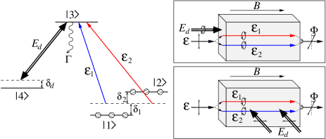
Figure 1: Level scheme of tripod atoms interacting with weak probe ${\cal E}$ and strong driving $E_{d}$ fields. Upper inset: copropagating probe with circularly left- and right-polarized components ${\cal E}_{1,2}$, and driving $E_{d}$ fields pass through the atomic medium that is subject to the longitudinal magnetic field $B$. Lower inset: Perpendicular arrangement of the probe and driving fields, that is suitable for cold atomic gas.

We consider a near-resonant interaction of two optical fields with a medium of atoms with tripod configuration of levels (Fig. 1). The medium is subject to a longitudinal magnetic field $B$ that removes the degeneracy of the ground state sublevels. The Zeeman shift of levels $\,|1\rangle$ and $\,|2\rangle$ is given by $\hbar\Delta=\mu_{\rm B}M_{F}g_{F}B$, where $\mu_{\rm B}$ is the Bohr magneton, $g_{F}$ is the gyromagnetic factor and $M_{F}=\pm 1$ is the magnetic quantum number of the corresponding state. All the atoms are assumed to be optically pumped to the states $\,|1\rangle$ and $\,|2\rangle$ which thus have the same incoherent populations equal to $1/2$. A linearly polarized weak (quantum) probe field ${\cal E}$ has a carrier frequency $\omega_{p}$ and wavevector $k_{p}$ parallel to the magnetic field direction. Its two circularly left- and right-polarized components ${\cal E}_{1,2}$ act on the atomic transitions $\,|1\rangle\to\,|3\rangle$ and $\,|2\rangle\to\,|3\rangle$, with the detunings $\delta_{1,2}=\omega_{p}-\omega_{31}^{0}-k_{p}v\mp\Delta$, where $\omega_{31}^{0}=\omega_{32}^{0}$ is the frequency of the unshifted atomic resonance and $k_{p}v$ is the Doppler shift for the atoms having velocity $v$ along the probe field propagation direction. A strong classical cw field $E_{d}$, having frequency $\omega_{d}$ and wavevector $k_{d}\simeq k_{p}$, is driving the atomic transition $\,|3\rangle\leftrightarrow\,|4\rangle$ with the Rabi frequency $\Omega_{d}=\wp_{34}E_{d}/\hbar$, where $\wp_{\mu\nu}$ is the dipole matrix element on the transition $\,|\mu\rangle\to\,|\nu\rangle$. In the collinear Doppler-free geometry shown in Fig. 1, upper inset, the driving field has to be circularly left or right polarized, in order to couple to a single magnetic sublevel $\,|4\rangle$. Its Zeeman shift $\hbar\Delta^{\prime}=\mu_{\rm B}M_{F^{\prime}}g_{F^{\prime}}B$ is incorporated in the detuning of the driving field via $\delta_{d}=\omega_{d}-\omega_{34}^{0}-k_{d}v+\Delta^{\prime}$, where $\omega_{34}^{0}$ is the atomic resonance frequency for zero magnetic field. Note that in the case of cold atomic sample (Doppler broadening of the atomic resonance is smaller than the ground-state spin relaxation rate), one can employ the perpendicular geometry of Fig. 1, lower inset, where the driving field is linearly $\pi$ polarized while the Zeeman shift of level $\,|4\rangle$ vanishes, $\Delta^{\prime}=0$ since $M_{F^{\prime}}=0$.

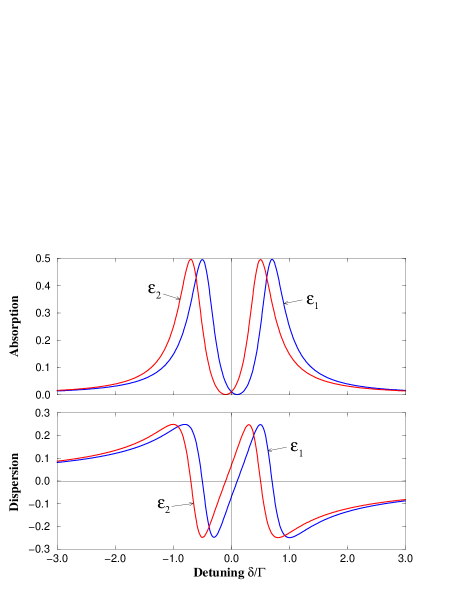
Figure 2: Absorption and dispersion spectra ($\delta=\omega_{p}-\omega_{31}^{0}$) for the ${\cal E}_{1}$ and ${\cal E}_{2}$ components of the probe in the presence of a strong driving ($\Omega_{d}=0.6\Gamma$) and a weak magnetic ($\Delta=0.1\Gamma$) fields, in units of the linear resonant absorption coefficient $a_{0}$.

To illustrate the scheme, we plot in Fig. 2 the absorption and dispersion spectra of the two components of the probe field ${\cal E}$ for the case $\delta_{d}=0$. In the presence of magnetic field, the spectra for the ${\cal E}_{1}$ and ${\cal E}_{2}$ are shifted with respect to each other by the amount equal to the Zeeman shift $2\Delta$. When the probe field is resonant with the unshifted ($\Delta=0$) atomic transitions, $\omega_{p}=\omega_{31}^{0}=\omega_{32}^{0}$, due to the steep and approximately linear slope of the dispersion in the vicinity of $\delta_{1,2}=0$, upon propagating through the medium the two components of the probe experience equal and opposite phase shifts $\phi_{1}=-\phi_{2}$ which results in a net polarization rotation of the field, $\Phi=\frac{1}{2}(\phi_{2}-\phi_{1})$. If the Zeeman shift is small compared to the width of the EIT window for both components of the probe, the absorption remains much smaller than the phase shift. Thus, a weak magnetic field can induce an appreciable polarization rotation accompanied by negligible absorption, allowing for extremely sensitive magnetometry (Sec. III). In addition to the large linear phase shift, each component experiences a nonlinear cross-phase modulation. Although this cross-phase modulation is typically small compared to the linear phase modulation, it is nevertheless several orders of magnitude larger than that in conventional media imam . It can therefore be used for quantum information applications based on photon-photon interaction and entanglement (Sec. IV).

Let us now consider the scheme more quantitatively. We describe the medium using collective slowly varying atomic operators $\hat{\sigma}_{\mu\nu}(z,t)=\frac{1}{N_{z}}\sum_{j=1}^{N_{z}}\,|\mu_{j}\rangle\langle\nu_{j}|\,$, averaged over small but macroscopic volume containing many atoms $N_{z}=(N/L)dz\gg 1$ around position $z$, where $N$ is the total number of atoms and $L$ is the length of the medium fllk . The two components of the quantum probe field are described by the corresponding field operators $\hat{\cal E}_{1,2}$. In a frame rotating with the probe and driving field frequencies, the interaction Hamiltonian has the following form

$$H = \hbar\frac{N}{L}\int_{0}^{L}dz[\delta_{1}\hat{\sigma}_{11}+\delta_{2}\hat{\sigma}_{22}+\delta_{d}\hat{\sigma}_{44}$$ (1)

$$\;\;\;\;\;\;\;\;\;\;-g(\hat{\cal E}_{1}\hat{\sigma}_{31}+\hat{\cal E}_{2}\hat{\sigma}_{32})-\Omega_{d}\hat{\sigma}_{34}+{\rm H.c.}].$$

Here $g=\wp_{31}\sqrt{\omega_{p}/(2\hbar\epsilon_{0}AL)}$, with $A$ being the cross-sectional area of the probe field, is the atom-field coupling constant, which is the same for both circular components $\hat{\cal E}_{1,2}$ due to the symmetry of the system ($|\wp_{31}|=|\wp_{32}|$ while the opposite signs of the Clebsch-Gordan coefficients on the transitions $\,|1\rangle\to\,|3\rangle$ and $\,|2\rangle\to\,|3\rangle$ can be incorporated into the atomic eigenstate via the transformation $\,|1\rangle\to e^{i\pi}\,|1\rangle$). Using the slowly varying envelope approximation, we obtain the following propagation equations for the quantum field operators

$$\left(\frac{\partial}{\partial t}+c\frac{\partial}{\partial z}\right)\hat{\cal E}_{1}(z,t) = igN\hat{\sigma}_{13},$$ (2a)

$$\left(\frac{\partial}{\partial t}+c\frac{\partial}{\partial z}\right)\hat{\cal E}_{2}(z,t) = igN\hat{\sigma}_{23}.$$ (2b)

The equations for the atomic coherences are given by

$$\frac{\partial}{\partial t}\hat{\sigma}_{12} = [i(\delta_{1}-\delta_{2})-\gamma_{c}]\hat{\sigma}_{12}-ig\hat{\cal E}_{1}\hat{\sigma}_{32}+ig\hat{\cal E}_{2}^{\dagger}\hat{\sigma}_{13}+\hat{F}_{12},$$ (3a)

$$\frac{\partial}{\partial t}\hat{\sigma}_{13} = \left(i\delta_{1}-\frac{\Gamma}{2}\right)\hat{\sigma}_{13}+ig\hat{\cal E}_{1}(\hat{\sigma}_{11}-\hat{\sigma}_{33})+ig\hat{\cal E}_{2}\hat{\sigma}_{12}+i\Omega_{d}\hat{\sigma}_{14}+\hat{F}_{13},$$ (3b)

$$\frac{\partial}{\partial t}\hat{\sigma}_{14} = [i(\delta_{1}-\delta_{d})-\gamma_{c}]\hat{\sigma}_{14}-ig\hat{\cal E}_{1}\hat{\sigma}_{34}+i\Omega_{d}^{*}\hat{\sigma}_{13}+\hat{F}_{14},$$ (3c)

$$\frac{\partial}{\partial t}\hat{\sigma}_{23} = \left(i\delta_{2}-\frac{\Gamma}{2}\right)\hat{\sigma}_{23}+ig\hat{\cal E}_{2}(\hat{\sigma}_{22}-\hat{\sigma}_{33})+ig\hat{\cal E}_{1}\hat{\sigma}_{21}+i\Omega_{d}\hat{\sigma}_{24}+\hat{F}_{23},$$ (3d)

$$\frac{\partial}{\partial t}\hat{\sigma}_{24} = [i(\delta_{2}-\delta_{d})-\gamma_{c}]\hat{\sigma}_{24}-ig\hat{\cal E}_{2}\hat{\sigma}_{34}+i\Omega_{d}^{*}\hat{\sigma}_{23}+\hat{F}_{24},$$ (3e)

$$\frac{\partial}{\partial t}\hat{\sigma}_{34} = -\left(i\delta_{d}+\frac{\Gamma}{2}\right)\hat{\sigma}_{34}-ig\hat{\cal E}_{1}^{\dagger}\hat{\sigma}_{14}-ig\hat{\cal E}_{2}^{\dagger}\hat{\sigma}_{24}+i\Omega_{d}^{*}(\hat{\sigma}_{33}-\hat{\sigma}_{44})+\hat{F}_{34},$$ (3f)

where $\gamma_{c}$ is the ground state coherence (spin) relaxation rate, $\Gamma$ is the decay rate of the excited state $\,|3\rangle$ and $\hat{F}_{\mu\nu}$ are $\delta$-correlated noise operators associated with the relaxation.

We now outline the solution of Eqs. (3) in the weak field limit. To this end, we assume that the Rabi frequencies $g{\cal E}_{1,2}$ of the quantum fields are much smaller than $\Omega_{d}$ and the number of photons in $\hat{\cal E}_{1,2}$ is much less than the number of atoms, therefore $\hat{\sigma}_{11}=\hat{\sigma}_{22}\simeq{\mathbf{1}}/2$ while $\hat{\sigma}_{33}=\hat{\sigma}_{44}=\hat{\sigma}_{34}\simeq 0$. We may thus treat the atomic equations perturbatively in the small parameters $g\hat{\cal E}_{1,2}/\Omega_{d}$. In the first order, from (3b) and (3d) we have

$$\hat{\sigma}_{14}^{(1)}=-\frac{g\hat{\cal E}_{1}}{2\Omega_{d}},\;\;\;\hat{\sigma}_{24}^{(1)}=-\frac{g\hat{\cal E}_{2}}{2\Omega_{d}}.$$

Substituting these into (3c) and (3e), and neglecting for now the spin relaxation, we obtain

$$\hat{\sigma}_{13}^{(1)} = \left[\frac{\partial}{\partial t}-i(\delta_{1}-\delta_{d})\right]\frac{ig\hat{\cal E}_{1}}{2|\Omega_{d}|^{2}}\simeq\frac{g\hat{\cal E}_{1}(\delta_{1}-\delta_{d})}{2|\Omega_{d}|^{2}},$$

$$\hat{\sigma}_{23}^{(1)} = \left[\frac{\partial}{\partial t}-i(\delta_{2}-\delta_{d})\right]\frac{ig\hat{\cal E}_{2}}{2|\Omega_{d}|^{2}}\simeq\frac{g\hat{\cal E}_{2}(\delta_{2}-\delta_{d})}{2|\Omega_{d}|^{2}}.$$

In these equations, the last equalities result from the adiabatic approximation, i.e., we assume that the probe pulse changes slowly enough so that the atoms follow the field adiabatically. Quantitatively, the adiabatic evolution requires that the rate of change of the probe field, $\max[\partial_{t}{\cal E}/{\cal E}]\sim T_{p}^{-1}$, where $T_{p}$ is the temporal width of the pulse, should be smaller than any transition rate between the system’s eigenstates, so that no nonresonant transition is induced messiah ; harris .

We next write Eq. (3a) in an integral form and perform the integration,

$$\hat{\sigma}_{12}=\frac{g\hat{\cal E}_{1}\hat{\sigma}_{32}^{(1)}-g\hat{\cal E}_{2}^{\dagger}\hat{\sigma}_{13}^{(1)}}{i\gamma_{c}-2\Delta}\left[1-\alpha e^{-i(2\Delta-i\gamma_{c})t}\right],$$

where $\alpha\simeq[1+(T_{p}\Delta)^{2}]^{-1}$ is the adiabaticity parameter. Thus in the adiabatic limit $T_{p}\gg|\Delta|^{-1}$, as well as for times $t\gg\gamma_{c}^{-1}$ (for any $\Delta$), the term proportional to $\alpha$ vanishes. Substituting the above expressions into

$$\hat{\sigma}_{14} = -\frac{g\hat{\cal E}_{1}}{2\Omega_{d}}-\frac{g\hat{\cal E}_{2}}{\Omega_{d}}\hat{\sigma}_{12}-\frac{i}{\Omega_{d}}\left[\left(\frac{\partial}{\partial t}-i\delta_{1}+\frac{\Gamma}{2}\right)\hat{\sigma}_{13}^{(1)}-\hat{F}_{13}\right],$$

$$\hat{\sigma}_{24} = -\frac{g\hat{\cal E}_{2}}{2\Omega_{d}}-\frac{g\hat{\cal E}_{1}}{\Omega_{d}}\hat{\sigma}_{21}-\frac{i}{\Omega_{d}}\left[\left(\frac{\partial}{\partial t}-i\delta_{2}+\frac{\Gamma}{2}\right)\hat{\sigma}_{23}^{(1)}-\hat{F}_{23}\right],$$

after some algebra, we finally arrive at the following set of equations

$$\hat{\sigma}_{13} = -\frac{i}{\Omega_{d}^{*}}\left[\frac{\partial}{\partial t}-i(\delta_{1}-\delta_{d})+\gamma_{c}\right]\hat{\sigma}_{14}+\frac{i}{\Omega_{d}^{*}}\hat{F}_{14},$$ (4a)

$$\hat{\sigma}_{14} = -\frac{g\hat{\cal E}_{1}}{2\Omega_{d}}\left[1+\frac{(\delta_{1}+i\Gamma/2)(\delta_{1}-\delta_{d})}{|\Omega_{d}|^{2}}+\frac{g^{2}\hat{I}_{2}2\Delta}{|\Omega_{d}|^{2}(i\gamma_{c}-2\Delta)}\right]+\frac{i}{\Omega_{d}}\hat{F}_{13},$$ (4b)

$$\hat{\sigma}_{23} = -\frac{i}{\Omega_{d}^{*}}\left[\frac{\partial}{\partial t}-i(\delta_{2}-\delta_{d})+\gamma_{c}\right]\hat{\sigma}_{24}+\frac{i}{\Omega_{d}^{*}}\hat{F}_{24},$$ (4c)

$$\hat{\sigma}_{24} = -\frac{g\hat{\cal E}_{2}}{2\Omega_{d}}\left[1+\frac{(\delta_{2}+i\Gamma/2)(\delta_{2}-\delta_{d})}{|\Omega_{d}|^{2}}-\frac{g^{2}\hat{I}_{1}2\Delta}{|\Omega_{d}|^{2}(i\gamma_{c}+2\Delta)}\right]+\frac{i}{\Omega_{d}}\hat{F}_{23},$$ (4d)

where $\hat{I}_{j}\equiv\hat{\cal E}_{j}^{\dagger}\hat{\cal E}_{j}$ is the dimensionless intensity (photon-number) operator for the $j$th field.

From now on we focus on the case of $\omega_{p}=\omega_{31}^{0}=\omega_{32}^{0}$. Substituting Eqs. (4) into Eqs. (2), the equations of motion for quantum fields are obtained as

$$\left[\frac{\partial}{\partial z}+\frac{1}{v_{g}^{(1)}}\frac{\partial}{\partial t}\right]\hat{\cal E}_{1} = -\kappa_{1}\hat{\cal E}_{1}-i(\Delta+\Delta_{d})(s_{1}-\eta_{1}\hat{I}_{2})\hat{\cal E}_{1}+\hat{\cal F}_{1},$$ (5a)

$$\left[\frac{\partial}{\partial z}+\frac{1}{v_{g}^{(2)}}\frac{\partial}{\partial t}\right]\hat{\cal E}_{2} = -\kappa_{2}\hat{\cal E}_{2}+i(\Delta-\Delta_{d})(s_{2}-\eta_{2}\hat{I}_{1})\hat{\cal E}_{2}+\hat{\cal F}_{2},$$ (5b)

where $\Delta_{d}=\omega_{d}-\omega_{34}^{0}+\Delta^{\prime}$ is the driving field detuning,

$$\kappa_{1,2} = \frac{Ng^{2}}{2c|\Omega_{d}|^{2}}\left[\gamma_{c}+\frac{\Gamma(\Delta\pm\Delta_{d})^{2}}{|\Omega_{d}|^{2}}\right],$$

$$s_{1,2} = \frac{Ng^{2}}{2c|\Omega_{d}|^{2}}\left[1+\frac{\Delta(\Delta\pm\Delta_{d})}{|\Omega_{d}|^{2}}\right]$$

are, respectively, the linear absorption and phase modulation coefficients,

$$\eta_{1,2}=\frac{Ng^{4}2\Delta}{2c|\Omega_{d}|^{4}(2\Delta\mp i\gamma_{c})}$$

are the cross-coupling coefficients, $v_{g}^{(1,2)}=(1/c+s_{1,2})^{-1}$ are the group velocities of the corresponding fields, and $\hat{\cal F}_{1,2}$ are the noise operators having the properties ScZub

$$\langle\hat{\cal F}_{i}(z)\rangle=\langle\hat{\cal F}_{i}(z)\hat{\cal F}_{i}(z^{\prime})\rangle = \langle\hat{\cal F}_{i}^{\dagger}(z)\hat{\cal F}_{i}^{\dagger}(z^{\prime})\rangle=0,$$

$$\langle\hat{\cal F}_{i}(z)\hat{\cal F}_{j}^{\dagger}(z^{\prime})\rangle = 2\kappa_{i}\delta_{ij}\delta(z-z^{\prime}).$$

In deriving Eqs. (5), we have assumed that the usual EIT conditions $|\Omega_{d}|^{2}\gg(\Delta\pm\Delta_{d})k_{p,d}\bar{v},\gamma_{c}(\Gamma+k_{p,d}\bar{v})$, where $\bar{v}$ is the mean thermal atomic velocity, are satisfied, allowing us to neglect the Doppler induced absorption. On the other hand, since the terms containing $k_{p}v$ enter Eqs. (4) linearly, the net phase-shift of the quantum fields, due to the Doppler shifts of the atomic resonance frequencies, averages to zero. Note also that if states $\,|1\rangle$, $\,|2\rangle$ and $\,|4\rangle$ belong to different hyperfine components of a common ground state, the frequencies $\omega_{p}$ and $\omega_{d}$ of the optical fields differ from each other by at most a few GHz, $\omega_{p}-\omega_{d}\simeq\omega_{41}^{0}\ll\omega_{p,d}$. Then, as seen from Eqs. (4), the difference $(k_{p}-k_{d})v$ in the Doppler shifts of the atomic resonances $\,|1\rangle,\,|2\rangle\to\,|3\rangle$ and $\,|4\rangle\to\,|3\rangle$ is negligible.

When $\Delta(\Delta\pm\Delta_{d})\ll|\Omega_{d}|^{2}$, the group velocities of $\hat{\cal E}_{1}$ are $\hat{\cal E}_{2}$ are practically the same, $v_{g}^{(1,2)}\simeq v_{g}$. Expressing the atom-field coupling constant $g$ through the linear resonant absorption coefficient $a_{0}=\wp_{13}^{2}\omega_{p}\rho/(\hbar c\epsilon_{0}\Gamma)$ for the transitions $\,|1\rangle,\,|2\rangle\to\,|3\rangle$ as $Ng^{2}=a_{0}c\Gamma/2$ and assuming that the density of atoms $\rho=N/(AL)$ is large enough so that $a_{0}c\Gamma\gg 4|\Omega_{d}|^{2}$, we have $v_{g}\simeq 4|\Omega_{d}|^{2}/(a_{0}\Gamma)\ll c$. Then the solution of Eqs. (5) can be expressed in terms of the retarded time $\tau=t-z/v_{g}$ as

$$\hat{\cal E}_{1}(z,t) = \hat{\cal E}_{1}(0,\tau)\exp\left[-\kappa_{1}z+i\hat{\phi}_{1}(z,0,t)\right]+\int_{0}^{z}dz^{\prime}\hat{\cal F}_{1}(z^{\prime})\exp\left[-\kappa_{1}(z-z^{\prime})+i\hat{\phi}_{1}(z,z^{\prime},t)\right],$$ (6a)

$$\hat{\cal E}_{2}(z,t) = \hat{\cal E}_{2}(0,\tau)\exp\left[-\kappa_{2}z+i\hat{\phi}_{2}(z,0,t)\right]+\int_{0}^{z}dz^{\prime}\hat{\cal F}_{2}(z^{\prime})\exp\left[-\kappa_{2}(z-z^{\prime})+i\hat{\phi}_{2}(z,z^{\prime},t)\right].$$ (6b)

where the phase operators are given by

$$\hat{\phi}_{1}(z,z^{\prime},t) = -s_{1}(\Delta+\Delta_{d})(z-z^{\prime})+\eta_{1}(\Delta+\Delta_{d})\int_{z^{\prime}}^{z}dz^{\prime\prime}\hat{I}_{2}(z^{\prime\prime},\tau+z^{\prime\prime}/v_{g}),\;$$

$$\hat{\phi}_{2}(z,z^{\prime},t) = s_{2}(\Delta-\Delta_{d})(z-z^{\prime})-\eta_{2}(\Delta-\Delta_{d})\int_{z^{\prime}}^{z}dz^{\prime\prime}\hat{I}_{1}(z^{\prime\prime},\tau+z^{\prime\prime}/v_{g}).\;$$

These are the central equations of this paper. The first terms in Eqs. (6) describe the linear attenuation and the phase shift of the corresponding quantum field $\hat{\cal E}_{1,2}$ upon propagating through the medium, while the second terms account for the noise contribution. Note that although the expectation values of the field operators decay, yet slowly, with the propagation, due to the presence of the noise operators, their commutators are preserved ScZub . We emphasize again that Eqs. (6) are obtained within the weak field and adiabatic approximations.

In the following section we explore the classical limit of Eqs. (6) for the purpose of sensitive magnetometry. In Sec. IV we study the quantum dynamics of the system and show that our scheme is capable of realizing strong nonlinear interaction and entanglement between two tightly focused quantum fields at the single-photon level.

III Optical magnetometer

Let us consider the classical limit of Eqs. (6), by replacing the operators $\hat{\cal E}_{1,2}$ with the corresponding c-numbers ${\mathcal{E}}_{1,2}$ and dropping the noise terms. The equations for the two circularly polarized components of the cw probe field have the form

$${\mathcal{E}}_{1}(z) = {\mathcal{E}}_{1}(0)e^{-\kappa_{1}z}e^{i\phi_{1}(z)},$$ (7a)

$${\mathcal{E}}_{2}(z) = {\mathcal{E}}_{2}(0)e^{-\kappa_{2}z}e^{i\phi_{2}(z)},$$ (7b)

where the absorption coefficients and phase shifts can be expressed through the group velocity $v_{g}$ as

$$\kappa_{1,2} = \frac{\gamma_{c}}{v_{g}}+\frac{\Gamma(\Delta\pm\Delta_{d})^{2}}{v_{g}|\Omega_{d}|^{2}},$$ (8a)

$$\phi_{1}(z) = -\frac{\Delta+\Delta_{d}}{v_{g}}z-\frac{\Delta(\Delta+\Delta_{d})^{2}}{v_{g}|\Omega_{d}|^{2}}z$$ (8b)

$$+\frac{\Delta+\Delta_{d}}{v_{g}}\frac{g^{2}I_{2}(0)}{|\Omega_{d}|^{2}}\frac{1-e^{-2k_{2}z}}{2k_{2}},$$

$$\phi_{2}(z) = \frac{\Delta-\Delta_{d}}{v_{g}}z+\frac{\Delta(\Delta-\Delta_{d})^{2}}{v_{g}|\Omega_{d}|^{2}}z$$ (8c)

$$-\frac{\Delta-\Delta_{d}}{v_{g}}\frac{g^{2}I_{1}(0)}{|\Omega_{d}|^{2}}\frac{1-e^{-2k_{1}z}}{2k_{1}}.$$

When the absorption is small, $\kappa_{1,2}z\ll 1$, $z\in\{0,L\}$, which requires that $v_{g}/\gamma_{c}\gg L$ and $\Delta^{2}+\Delta_{d}^{2}\lesssim\gamma_{c}|\Omega_{d}|^{2}/\Gamma$, the polarization rotation of the probe field $\Phi(z)=\frac{1}{2}[\phi_{2}(z)-\phi_{1}(z)]$ is given by

$$\Phi(z)=\frac{\Delta}{v_{g}}z+\frac{\Delta(\Delta^{2}+\Delta_{d}^{2})}{v_{g}|\Omega_{d}|^{2}}z+\frac{\Delta}{v_{g}}\frac{g^{2}I(0)}{|\Omega_{d}|^{2}}z,$$ (9)

where $I(0)=I_{1}(0)=I_{2}(0)$ since the probe is linearly polarized at the entrance to the medium. In Eq. (9), the first term is linear in the magnetic field while the second term has a cubic dependence on the field strength. Here we focus our attention on the measurement of dc magnetic fields employing the dominating linear term. We wish, however, to point out that the presence of the cubic term may facilitate the detection of ac fields oscillating slowly compared to the bandwidth of the magnetometer, which is limited by the bandwidth of the EIT window quantbw

$$\delta\omega\leq\frac{|\Omega_{d}|^{2}}{\Gamma}\frac{k_{p}}{\sqrt{3\pi\rho L}}.$$ (10)

Then the spectrum of $\Phi$, along with the fundamental frequency of the magnetic field, will also contain its third harmonic which, for very small frequencies, may be easier to detect kominis . This issue is beyond the scope of this paper and will be addressed elsewhere. Finally, the last term of Eq. (9), being proportional to the product of the magnetic field strength and probe intensity, is a consequence of Kerr-type nonlinear interaction between ${\mathcal{E}}_{1}$ and ${\mathcal{E}}_{2}$, which is the subject of the following section.

We consider a magnetometer setup in the “balanced polarimeter” arrangement budker_rev , in which, at the exit from the medium $z=L$, a polarizing beam splitter oriented at $\pi/4$ to the input polarizer [$\Phi(0)=0$] is used as an analyzer. Then the detector signal $S$ is represented by the difference of photocounts in the two channels of the analyzer

$$S=2n_{\rm in}e^{-2\kappa L}\sin[\Phi(L)]\cos[\Phi(L)],$$ (11)

where $n_{\rm in}=P_{\rm in}t_{m}/(\hbar\omega_{p})=2I(0)ct_{m}/L$, with $P_{\rm in}$ being the input power of the probe, is the number of photons passing through the medium during the measurement time $t_{m}$. For simplicity, we neglect the difference between the absorption coefficients for the circularly left- and right-polarized components, $\kappa_{1}\simeq\kappa_{2}=\kappa$, which amounts to neglecting the ellipticity of the output field ($\varepsilon\simeq 1$) since $\sqrt{1-\varepsilon^{2}}=2\Gamma\Delta\Delta_{d}L/(v_{g}|\Omega_{d}|^{2})\ll 1$.

The most important characteristic of a magnetometer is its sensitivity to weak magnetic fields, which is limited by the measurement noise. The smallest detectable magnetic field $B_{\rm min}$ can be defined as being the field for which the signal is equal to the noise. In our system, the total noise ${\cal N}={\cal N}_{\rm at}+{\cal N}_{\rm shot}$ has two contributions, atomic noise ${\cal N}_{\rm at}$ and photon counting shot-noise ${\cal N}_{\rm shot}$. The atomic contribution is due to the spontaneous photons reaching the detector during the measurement time,

$${\cal N}_{\rm at}=\Gamma\langle\hat{\sigma}_{33}\rangle Nt_{m}\frac{A}{4\pi L^{2}},$$

where the detector area is assumed to be equal to $A$. For vanishing magnetic field $\Delta<\gamma_{c}$, we have $\langle\hat{\sigma}_{33}\rangle N\simeq a_{0}c\Gamma\gamma_{c}^{2}I(0)/(4|\Omega_{d}|^{4})$ and the atomic noise is given by

$${\cal N}_{\rm at}=\frac{a_{0}\Gamma^{2}\gamma_{c}^{2}A}{32\pi|\Omega_{d}|^{4}L}n_{\rm in}.$$

For physically realistic parameters (see below), the atomic noise term is small compared to the photon counting shot-noise flscl

$${\cal N}_{\rm shot}=\sqrt{\frac{1+e^{-2\kappa L}}{2}n_{\rm in}}\leq\sqrt{n_{\rm in}}.$$

In the limit of weak magnetic field, retaining only the linear in magnetic field term, from $S\simeq 2n_{\rm in}\Phi\geq{\cal N}_{\rm shot}$ we obtain

$$B_{\rm min}\geq\frac{2\hbar|\Omega_{d}|^{2}}{g_{F}\mu_{B}a_{0}L\Gamma\sqrt{n_{\rm in}}}.$$ (12)

For realistic experimental parameters, $\omega_{p}=3\times 10^{15}$ rad/s, $\Gamma=10^{7}$ s^-1, $\rho=10^{13}$ cm^-3 ($a_{0}\simeq 10^{4}$ cm^-1), $|g_{F}|=1/2$, $\Omega_{d}\simeq\Gamma$, $L=10$ cm, $P_{\rm in}=1$ mW, $t_{m}=1$ s, the minimum detectable magnetic field $B_{\rm min}\lesssim 10^{-12}$ G, which is of the same order as that of butker ; scully-mor ; flscl . Thus, concerning the magnetometer sensitivity, our scheme is essentially equivalent to the one proposed in flscl , where an interferometric measurement of the magnetic field induced phase shift of a probe field, subject to EIT with $\Lambda$ atoms, was studied. Experimentally, however, measuring the polarization rotation of the probe, as suggested here, may be more practical than measuring its phase shift in the setup of flscl , which employs a Mach-Zehnder interferometer.

IV Cross-phase modulation

In order to rigorously describe the nonlinear interaction between the weak pulsed fields, we now turn to the fully quantum treatment of the system. When absorption is small enough to be neglected, from Eqs. (6) we have

$$\hat{\cal E}_{1}(z,t) = \hat{\cal E}_{1}(0,\tau)\exp[i\eta(\Delta+\Delta_{d})\hat{\cal E}_{2}^{\dagger}(0,\tau)\hat{\cal E}_{2}(0,\tau)z],$$

$$\hat{\cal E}_{2}(z,t) = \hat{\cal E}_{1}(0,\tau)\exp[-i\eta(\Delta-\Delta_{d})\hat{\cal E}_{1}^{\dagger}(0,\tau)\hat{\cal E}_{1}(0,\tau)z],$$

where the cross-phase modulation coefficient is given by $\eta=g^{2}/(v_{g}|\Omega_{d}|^{2})$ (assuming $\gamma_{c}\ll\Delta$), while the linear phase-modulation is incorporated into the field operators via the unitary transformations $\hat{\cal E}_{1}(z,t)\to\hat{\cal E}_{1}(z,t)e^{-is_{1}(\Delta+\Delta_{d})z}$ and $\hat{\cal E}_{2}(z,t)\to\hat{\cal E}_{2}(z,t)e^{is_{2}(\Delta-\Delta_{d})z}$. These traveling-wave electric fields can be expressed through single mode operators as $\hat{\cal E}_{j}(z,t)=\sum_{q}a_{j}^{q}(t)e^{iqz}$ ($j=1,2$), where $a_{j}^{q}$ is the annihilation operator for the field mode with the wavevector $k_{p}+q$. The single-mode operators $a_{j}^{q}$ and $a^{q\dagger}_{j}$ possess the standard bosonic commutation relations $[a_{i}^{q},a_{j}^{q^{\prime}\dagger}]=\delta_{ij}\delta_{qq^{\prime}}$. The continuum of modes scanned by $q\in\{-\delta q/2,\delta q/2\}$ is bounded by the EIT window via $\delta q\leq\delta\omega/c$ lukimam . The finite quantization bandwidth $\delta q$ for the field operators leads to the equal-time commutation relations

$$[\hat{\cal E}_{i}(z),\hat{\cal E}_{j}^{\dagger}(z^{\prime})]=\delta_{ij}\frac{L\delta q}{2\pi}{\rm sinc}\left[\delta q(z-z^{\prime})/2\right],$$

where ${\rm sinc}(x)=\sin(x)/x$.

Before proceeding, we note that Eqs. (13) are similar to the corresponding equations of Ref. lukimam , where the cross-phase modulation between two quantum fields was mediated by atoms with N configuration of levels imam , while the group velocity mismatch between the fields was compensated by using a second kind of $\Lambda$-atoms controlled by an additional driving field. In contrast, our scheme relies solely on an intra-atomic process employing only one driving field that causes simultaneous EIT for both fields and their cross-coupling. It is therefore deprived of complications associated with using mixtures of two isotopic species of atoms lukimam or invoking cavity QED techniques phphcav .

The most classical of all the quantum states is the coherent state. To compare the classical and quantum pictures, we therefore consider first the evolution of input wavepacket $\,|\psi_{\rm in}\rangle=\,|\alpha_{1}\rangle\otimes\,|\alpha_{2}\rangle$ composed of the multimode coherent states $\,|\alpha_{j}\rangle\equiv\Pi_{q}\,|\alpha_{j}^{q}\rangle$ ($j=1,2$). The states $\,|\alpha_{j}\rangle$ are the eigenstates of the input operators $\hat{\cal E}_{j}(0,t)$ at $z=0$ with the eigenvalues $\alpha_{j}(t)=\sum_{q}\alpha_{j}^{q}e^{-iqct}$: $\hat{\cal E}_{j}(0,t)\,|\alpha_{j}\rangle=\alpha_{j}(t)\,|\alpha_{j}\rangle$. Upon propagating through the medium, each pulse experiences a nonlinear cross-phase modulation. The expectation values for the fields are then obtained as

$$\langle\hat{\cal E}_{1}(z,t)\rangle = \alpha_{1}(\tau)\exp\left\{\left[e^{i\theta_{1}(z)}-1\right]\frac{2\pi|\alpha_{2}(\tau)|^{2}}{L\delta q}\right\},\;\;\;\;\;$$ (14a)

$$\langle\hat{\cal E}_{2}(z,t)\rangle = \alpha_{2}(\tau)\exp\left\{\left[e^{i\theta_{2}(z)}-1\right]\frac{2\pi|\alpha_{1}(\tau)|^{2}}{L\delta q}\right\},$$ (14b)

where $\theta_{1,2}(z)=\eta(\Delta_{d}\pm\Delta)L\delta qz/(2\pi)$. These equations are similar to those obtained for single-mode sami and multimode copropagating fields lukimam . They indicate that when the cross-phase modulation is large, upon propagating through the medium, the phases

$$2\pi\sin[\theta_{1,2}(z)]\frac{|\alpha_{2,1}(\tau)|^{2}}{L\delta q}$$

and amplitudes

$$\alpha_{1,2}(\tau)\exp\left\{-4\pi\sin^{2}[\theta_{1,2}(z)/2]\frac{|\alpha_{2,1}(\tau)|^{2}}{L\delta q}\right\}$$

of the quantum fields exhibit periodic collapses and revivals as $\theta_{1,2}(z)$ change from 0 to $2\pi$. In particular, when the phase-shift is maximal, $\theta_{1,2}=\pi/2$, the amplitude of the corresponding field is reduced by a factor of $r_{1,2}=\exp[-2\pi|\alpha_{2,1}|^{2}/(L\delta q)]$. On the other hand, the maximal dephasing of the multimode coherent field, $r_{1,2}=\exp[-4\pi|\alpha_{2,1}|^{2}/(L\delta q)]$, is attained for $\theta_{1,2}(z)=(2n+1)\pi$ ($n=0,1,2,\ldots$), where the phase shift is zero.

We have thus seen that the behavior of weak quantum fields is remarkably different from that of classical fields, as in the quantum regime the nonlinear phase shift is bounded between $\pm 2\pi|\alpha_{2,1}|^{2}/(L\delta q)$. Only in the limit of weak cross-phase modulation $\theta_{1,2}\ll 1$, the quantum Eqs. (14) reproduce the classical result

$$\langle\hat{\cal E}_{1,2}(z,t)\rangle=\alpha_{1,2}(\tau)\exp[i\eta(\Delta_{d}\pm\Delta)|\alpha_{2,1}(\tau)|^{2}z],$$

whereby the cross-phase shift grows linearly with the propagation distance and can attain large values when the field amplitudes are sufficiently high.

Let us now consider the input state $\,|\psi_{\rm in}\rangle=\,|1_{1}\rangle\otimes\,|1_{2}\rangle$, consisting of two single photon wavepackets $\,|1_{j}\rangle=\sum_{q}\xi_{j}^{q}a_{j}^{q\dagger}\,|0\rangle$ ($j=1,2$). The Fourier amplitudes $\xi_{j}^{q}$, normalized as $\sum_{q}|\xi_{j}^{q}|^{2}=1$, define the spatial envelopes $f_{j}(z)$ of the two pulses that initially (at $t=0$) are localized around $z=0$,

$$\langle 0|\,\hat{\cal E}_{j}(z,0)\,|1_{j}\rangle=\sum_{q}\xi_{j}^{q}e^{iqz}=f_{j}(z).$$

In free space, $\hat{\cal E}_{j}(z,t)=\hat{\cal E}_{j}(0,\tau)$ with $\tau=t-z/c$, and we have $\langle 0|\,\hat{\cal E}_{j}(z,t)\,|1_{j}\rangle=f_{j}(z-ct)$. The state of the system at any time can be represented as

$$\,|\psi(t)\rangle=\sum_{q,q^{\prime}}\xi_{12}^{qq^{\prime}}(t)\,|1_{1}^{q}\rangle\,|1_{2}^{q^{\prime}}\rangle,$$ (15)

from where it is apparent that $\xi_{12}^{qq^{\prime}}(0)=\xi_{1}^{q}\xi_{2}^{q^{\prime}}$.

Since for the photon-number states the expectation values of the field operators vanish, all the information about the state of the system is contained in the intensities of the corresponding fields

$$\langle\hat{I}_{j}(z,t)\rangle=\langle\psi_{\rm in}|\,\hat{\cal E}_{j}^{\dagger}(z,t)\hat{\cal E}_{j}(z,t)\,|\psi_{\rm in}\rangle,$$ (16)

and their “two-photon wavefunction” ScZub ; lukimam

$$\Psi_{ij}(z,t;z^{\prime},t^{\prime})=\langle 0|\,\hat{\cal E}_{j}(z^{\prime},t^{\prime})\hat{\cal E}_{i}(z,t)\,|\psi_{\rm in}\rangle.$$ (17)

The physical meaning of $\Psi_{ij}$ is a two-photon detection amplitude, through which one can express the second-order correlation function $G^{(2)}_{ij}=\Psi_{ij}^{*}\Psi_{ij}$ ScZub . The knowledge of the two-photon wavefunction allows one to calculate the amplitudes $\xi_{12}^{qq^{\prime}}$ of state vector (15) via the two dimensional Fourier transform of $\Psi_{ij}$ at $t=t^{\prime}$:

$$\xi_{ij}^{qq^{\prime}}(t)=\frac{1}{L^{2}}\int\!\!\!\int dzdz^{\prime}\Psi_{ij}(z,z^{\prime},t)e^{-iqz}e^{-iq^{\prime}z^{\prime}}.$$ (18)

We first calculate the expectation values of the intensities $\langle\hat{I}_{j}(z,t)\rangle$ by substituting the operator solution (13) into (16),

$$\langle\hat{I}_{j}(z,t)\rangle=|f_{j}(-c\tau)|^{2}=|f_{j}(zc/v_{g}-ct)|^{2},$$ (19)

where $\tau=t-z/v_{g}$ for $0\leq z<L$. This equation indicates that upon entering the medium, as the group velocities of the pulses are slowed down to $v_{g}\ll c$, their spatial envelopes are compressed by a factor of $c/v_{g}$ fllk . Outside the medium, at $z\geq L$ and accordingly $\tau=t-L/v_{g}-(z-L)/c$, we have $\langle\hat{I}_{j}(z,t)\rangle=|f_{j}(z+L(c/v_{g}-1)-ct)|^{2}$, which shows that the propagation velocity and the pulse envelopes are restored to their free-space values.

Consider next the two photon wavefunction $\Psi_{ij}$. After the interaction, at $z,z^{\prime}\geq L$, we have the general expression

$$\Psi_{ij}(z,t;z^{\prime},t^{\prime}) = f_{i}(-c\tau)f_{j}(-c\tau^{\prime})\left\{1+\frac{f_{j}(-c\tau)}{f_{j}(-c\tau^{\prime})}{\rm sinc}\left[\frac{\delta\omega}{2}(\tau-\tau^{\prime})\right]\left(e^{i\theta_{i}(L)}-1\right)\right\},$$ (20)

where, as before, $\tau=t-L/v_{g}-(z-L)/c$ and similarly for $\tau^{\prime}$. For quantum information applications, it makes sense to consider the relatively simple case of small magnetic field, such that $\Delta,\Delta^{\prime}\ll\Delta_{d}$, where the driving field detuning $\Delta_{d}=\omega_{d}-\omega_{34}^{0}$ satisfies $|\Delta_{d}|<\delta\omega/2$. We thus have $\theta_{1,2}\simeq\theta=\eta\Delta_{d}L^{2}\delta q/(2\pi)$. Then the equal-time ($t=t^{\prime}$) two-photon wavefunction reads

$$\Psi_{ij}(z,z^{\prime},t) = f_{i}[z+L(c/v_{g}-1)-ct]\>f_{j}[z^{\prime}+L(c/v_{g}-1)-ct]$$ (21)

$$\times\left\{1+\frac{f_{j}[z+L(c/v_{g}-1)-ct]}{f_{j}[z^{\prime}+L(c/v_{g}-1)-ct]}\>{\rm sinc}\left[\frac{\delta q}{2}(z^{\prime}-z)\right]\left(e^{i\theta}-1\right)\right\}.$$

For large enough spatial separation between the two photons, such that $|z^{\prime}-z|>\delta q^{-1}$ and therefore ${\rm sinc}[\delta q(z^{\prime}-z)/2]\simeq 0$, Eq. (21) yields

$$\Psi_{ij}(z,z^{\prime},t)\simeq f_{i}[z+L(c/v_{g}-1)-ct]\>f_{j}[z^{\prime}+L(c/v_{g}-1)-ct],$$

which indicates that no nonlinear interaction takes place between the photons, which emerge from the medium unchanged. This is due to the local character of the interaction described by the ${\rm sinc}$ function.

Consider now the opposite limit of $|z^{\prime}-z|\ll\delta q^{-1}$ and therefore ${\rm sinc}[\delta q(z^{\prime}-z)/2]\simeq 1$. Then for two narrow-band (Fourier limited) pulses with the duration $T_{p}\gg|z^{\prime}-z|/c$, one has $f_{j}(z)/f_{j}(z^{\prime})\simeq 1$, and Eq. (21) results in

$$\Psi_{ij}(z,z^{\prime},t) \simeq e^{i\theta}f_{i}[z+L(c/v_{g}-1)-ct]$$

$$\;\;\;\;\times f_{j}[z^{\prime}+L(c/v_{g}-1)-ct].$$

Thus, after the interaction, a pair of single photons acquires conditional phase shift $\theta$, which can exceed $\pi$ when

$$\left(\frac{\delta qL}{2\pi}\right)^{2}>\frac{v_{g}|\Omega_{d}|^{2}}{cg^{2}}.$$

To see this more clearly, we use Eq. (18) to calculate the amplitudes of the state vector $\,|\psi(t)\rangle$:

$$\xi_{ij}^{qq^{\prime}}(t)=e^{i\theta}\xi_{ij}^{qq^{\prime}}(0)\exp\{i(q+q^{\prime})[L(c/v_{g}-1)-ct]\}.$$ (22)

At the exit from the medium, at time $t\simeq L/v_{g}$, the second exponent in Eq. (22) can be neglected for all $q,q^{\prime}$ and the state of the system is given by

$$\,|\psi(L/v_{g})\rangle=e^{i\theta}\,|\psi_{\rm in}\rangle.$$ (23)

When $\theta=\pi$, this transformation corresponds to the truth table of the controlled-phase (cphase) logic gate between the two photons representing qubits. Together with the linear single-photon phase shifts (realizing single-qubit rotations), the cphase gate is said to be universal in the sense that it can realize arbitrary unitary transformation QCQI .

V Conclusions

In this paper, we have studied a propagation of weak probe field through an optically dense medium of coherently driven four-level atoms in a tripod configuration. We have presented a detailed semiclassical as well as quantum analysis of the system. One of the conclusions that emerged from this study is that optically dense vapors of tripod atoms can support ultrasensitive magneto-optical polarization rotation of the probe field and therefore have significant potential for improving the sensitivity of Faraday magnetometers to small magnetic fields. Another finding is that this system is capable of realizing a novel regime of symmetric, extremely efficient nonlinear interaction of two multimode single-photon pulses, whereby the combined state of the system acquires a large conditional phase shift that can easily exceed $\pi$. Thus our scheme may pave the way to photon-based quantum information applications, such as deterministic all-optical quantum computation, dense coding and teleportation QCQI .

References

• (1) S.E. Harris, Phys. Today 50(7), 36 (1997); E. Arimondo, in Progress in Optics, edited by E. Wolf, (Elsevier Science, Amsterdam, 1996), vol. 35, p. 257.
• (2) M.O. Scully and M.S. Zubairy, Quantum Optics (Cambridge University Press, Cambridge, UK, 1997).
• (3) L.V. Hau, S.E. Harris, Z. Dutton, and C.H. Behroozi, Nature (London) 397, 594 (1999); M.M. Kash, V.A. Sautenkov, A.S. Zibrov, L. Hollberg, G.R. Welch, M.D. Lukin, Yu. Rostovtsev, E.S. Fry, and M.O. Scully, Phys. Rev. Lett. 82, 5229 (1999); D. Budker, D.F. Kimball, S.M. Rochester, and V.V. Yashchuk, Phys. Rev. Lett. 83, 1767 (1999).
• (4) A.B. Matsko, Yu.V. Rostovtsev, H.Z. Cummins, and M.O. Scully, Phys. Rev. Lett. 84, 5752 (2000).
• (5) M. Fleischhauer and M.D. Lukin, Phys. Rev. Lett. 84, 5094 (2000); Phys. Rev. A 65, 022314 (2002).
• (6) D.F. Phillips, A. Fleischhauer, A. Mair, R.L. Walsworth, and M.D. Lukin, Phys. Rev. Lett. 86, 783 (2001); C. Liu, Z. Dutton, C.H. Behroozi, and L.V. Hau, Nature 409, 490 (2001).
• (7) A.V. Turukhin, V.S. Sudarshanam, M.S. Shahriar, J.A. Musser, B.S. Ham, and P.R. Hemmer, Phys. Rev. Lett. 88, 023602 (2002).
• (8) A. Andre and M.D. Lukin, Phys. Rev. Lett. 89, 143602 (2002); M. Bajcsy, A.S. Zibrov, M.D. Lukin, Nature 426, 638 (2003).
• (9) H. Schmidt and A. Imamoğlu, Opt. Lett. 21, 1936 (1996).
• (10) S.E. Harris and Y. Yamamoto, Phys. Rev. Lett. 81, 3611 (1998); S. Harris and L. Hau, Phys. Rev. Lett. 82, 4611 (1999).
• (11) F. Vewinger, M. Heinz, R.G. Fernandez, N.V. Vitanov, and K. Bergmann, Phys. Rev. Lett. 91, 213001 (2003).
• (12) K. Bergmann, H. Theuer, and B.W. Shore, Rev. Mod. Phys. 70, 1003 (1998).
• (13) E. Paspalakis, N.J. Kylstra, and P. Knight, Phys. Rev. A 65, 053808 (2002); E. Paspalakis and P. Knight, J Mod. Opt. 49, 87 (2002).
• (14) E. Paspalakis and Z. Kis, Opt. Lett. 27, 1836 (2002); Z. Kis and E. Paspalakis, Phys. Rev. A 68, 043817 (2003).
• (15) Yu.P. Malakyan, quant-ph/0112058.
• (16) D. Budker, W. Gawlik, D.F. Kimball, S.M. Rochester, V.V. Yashchuk, and A. Weis, Rev. Mod. Phys. 74(4), 1153 (2002).
• (17) D. Budker, V. Yashchuk, and M. Zolotorev, Phys. Rev. Lett. 81, 5788 (1998); D. Budker, D F. Kimball, S.M. Rochester, V.V. Yashchuk, and M. Zolotorev, Phys. Rev. A 62, 043403 (2000).
• (18) V.A. Sautenkov, M.D. Lukin, C.J. Bednar, I. Novikova, E. Mikhailov, M. Fleischhauer, V.L. Velichansky, G.R. Welch, and M.O. Scully, Phys. Rev. A 62, 023810 (2000); I. Novikova, A.B. Matsko, V.A. Sautenkov, V.L. Velichansky, G.R. Welch, and M.O. Scully, Opt. Lett. 25, 1651 (2000); I. Novikova, A.B. Matsko, and G.R. Welch, Opt. Lett. 26, 1016 (2001).
• (19) M.O. Scully and M. Fleischhauer, Phys. Rev. Lett. 69, 1360 (1992); M. Fleischhauer and M.O. Scully, Phys. Rev. A 49, 1973 (1994).
• (20) J. DuPont-Roc, S. Haroche, and C. Cohen-Tannoudji, Phys. Lett. A 28, 638 (1969); I. Kominis, T. Kornack, J. Allred, and M. Romalis, Nature (London) 422, 596 (2003).
• (21) M.A. Nielsen and I.L. Chuang, Quantum Computation and Quantum Information (Cambridge University Press, Cambridge, UK, 2000); A. Steane, Rep. Prog. Phys. 61, 117 (1998); C.H. Bennett and D.P. DiVincenzo, Nature 404, 247 (2000).
• (22) D. Loss and D.P. DiVincenzo, Phys. Rev. A 57, 120 (1998); B.E. Kane, Nature 393, 133 (1998).
• (23) J.I. Cirac and P. Zoller, Phys. Rev. Lett. 74, 4091 (1995); C.A. Sackett, D. Kielpinski, B.E. King, C. Langer, V. Meyer, C.J. Myatt, M. Rowe, Q.A. Turchette, W.M. Itano, D.J. Wineland, and C. Monroe, Nature 404, 256 (2000).
• (24) G.K. Brennen, C.M. Caves, P.S. Jessen, and I.H. Deutsch, Phys. Rev. Lett. 82, 1060 (1999).
• (25) E. Knill, R. Laflamme, and G.J. Milburn, Nature 409, 46 (2001); L.-M. Duan, M.D. Lukin, J.I. Cirac, and P. Zoller, Nature 414, 413 (2001).
• (26) Q.A. Turchette, C.J. Hood, W. Lange, H. Mabuchi, and H.J. Kimble, Phys. Rev. Lett. 75, 4710 (1995); A. Imamoglu, H. Schmidt, G. Woods, and M. Deutsch, Phys. Rev. Lett. 79, 1467 (1997); A. Rauschenbeutel, G. Nogues, S. Osnaghi, P. Bertet, M. Brune, J.M. Raimond, and S. Haroche, Phys. Rev. Lett. 83, 5166 (1999).
• (27) R.W. Boyd, Nonlinear Optics (Academic Press, San Diego, CA, 1992).
• (28) M.D. Lukin and A. Imamoğlu, Phys. Rev. Lett. 84, 1419 (2000).
• (29) S. Rebic, D. Vitali, C. Ottaviani, P. Tombesi, M. Artoni, F. Cataliotti, and R. Corbalan, quant-ph/0310148.
• (30) A. Messiah, Quantum Mechanics (Elsevier Science, New York, 1981).
• (31) M.D. Lukin, M. Fleischhauer, A.S. Zibrov, H.G. Robinson, V.L. Velichansky, L. Hollberg, and M.O. Scully, Phys. Rev. Lett. 79, 2959 (1997).
• (32) I. Kominis (private communications).
• (33) B.C. Sanders and G.J. Milburn, Phys. Rev. A 45, 1919 (1992).