A Model for Quantum Jumps in Magnetic Resonance Force Microscopy

Abstract

We propose a simple model which describes the statistical properties of quantum jumps in a single-spin measurement using the oscillating cantilever-driven adiabatic reversals technique in magnetic resonance force microscopy. Our computer simulations based on this model predict the average time interval between two consecutive quantum jumps and the correlation time to be proportional to the characteristic time of the magnetic noise and inversely proportional to the square of the magnetic noise amplitude.

I Introduction

Recent achievements in magnetic resonance force microscopy (MRFM) promise a single spin detection in the near future 1 . One may expect that single spin signal will represent a random sequence of quantum jumps. The important problem for the theory is modeling of quantum jumps in MRFM and the computation of their statistical characteristics. In this paper we propose a simple model which describes quantum jumps in MRFM single spin detection. We consider the oscillating cantilever-driven adiabatic reversals technique (OSCAR) which currently is the most promising approach for single spin detection 1 . In OSCAR the cantilever tip (CT) with a ferromagnetic particle oscillates, causing the periodic adiabatic reversals of the effective magnetic field on spin. The spin follows the effective magnetic field causing a tiny frequency shift of the CT vibrations which is measured.

In the second section we consider the Schrödinger dynamics of the CT-spin system which underlines our model of quantum jumps. In the third section we describe our model and present the results of the computer simulations. In Conclusion we discuss our results.

II Schrödinger dynamics of the CT-spin system

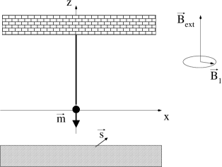
Figure 1: Single spin OSCAR MRFM setup. ${\vec{B}}_{ext}$ is the external permanent magnetic field; $B_{1}$ is the rotating rf field; ${\vec{m}}$ is the magnetic moment of the ferromagnetic particle; ${\vec{s}}$ is a spin near the surface of the sample.

We consider a vertical cantilever with a ferromagnetic particle attached to the CT and oscillating along the $x$-axis which is parallel to the surface of the sample. (See Fig. 1). The Hamiltonian of the CT-spin system in the system of coordinates which rotates with a circularly polarized rf field can be written as

$${\cal H}={{1}\over{2}}(p_{c}^{2}+x^{2}_{c})+\varepsilon S_{x}+2\eta x_{c}S_{z}+\Delta(\tau)S_{z}.$$

Here $p_{c}$ is the effective momentum of the CT, $x_{c}$ is its coordinate, the first term describes the effective energy of the CT; the second term describes the interaction between the spin and the rf field; the third term describes the interaction between the CT and the spin; and the last term describes the interaction between the spin and the random magnetic field which causes a deviation of spin from the effective magnetic field when the latter passes through the transverse $x-y$-plane 2 ; 3 . All quantities in (1) are dimensionless: $p_{c}$ and $x_{c}$ are expressed in terms of the “quantum units” $X_{0}$ and $P_{0}$

$$X_{0}=(\hbar\omega_{c}/k_{c})^{1/2},~{}P_{0}=\hbar/X_{0}.$$

The dimensionless parameters $\varepsilon$, $\eta$, and $\Delta(\tau)$ are defined as

$$\varepsilon=\gamma B_{1}/\omega_{c},~{}\eta=\gamma(\hbar/k_{c}\omega_{c})^{1/2}|\partial B_{z}(x)/\partial x|/2,$$

$$\Delta(\tau)=\gamma\Delta B_{z}(\tau)/\omega_{c},~{}\tau=\omega_{c}t.$$

Here $B_{z}$ is the $z$-component of the “regular magnetic field” which includes ${\vec{B}}_{ext}$ and the regular dipole-magnetic field produced by the ferromagnetic particle at the location of the spin; $\Delta B_{z}(\tau)$ is the $z$-component of the random field with zero average value; $\gamma$ is the magnitude of the spin gyromagnetic ratio: $k_{c}$ and $\omega_{c}$ are the effective spring constant and fundamental frequency of the CT; and $\tau$ is the dimensionless time.

Using the parameters presented in 1

$$\omega_{c}/2\pi=6.6kHz,~{}k_{c}=6\times 10^{-4}N/m,$$

$$B_{1}=0.3mT,~{}|\partial B_{z}(x)/\partial x|\approx 4.3\times 10^{5}T/m,$$

we can estimate all parameters in (1) except of $\Delta(\tau)$:

$$X_{0}=85fm,~{}P_{0}=1.2\times 10^{-21}Ns,~{}\eta=0.078,~{}\varepsilon=1270.$$

To simplify computer simulations we considered the function $\Delta(\tau)$ to be a random telegraph signal with two values $\pm\Delta$. The time interval between two consecutive “kicks” of $\Delta(\tau)$ was taken randomly from the interval $(\tau_{0}-\delta\tau,\tau_{0}+\delta\tau)$, with the average time interval, $\tau_{0}$, close to the Rabi period $\tau_{R}$

$$\tau_{R}=\omega_{c}(2\pi/\gamma B_{1})=2\pi/\varepsilon=4.95\times 10^{-3}.$$

We choose the initial state of the CT to be a coherent quasiclassical state, and the average spin to be pointed along the “regular” effective magnetic field with the components $(\varepsilon,0,2\eta x_{c})$.

Below we describe briefly the results of our computer simulations. Our simulations reveal the formation of a Schrödinger cat state for the CT: the probability distribution function $P(x,\tau)\equiv\Psi^{\dagger}(x,\tau)\Psi(x,\tau)$ splits into two peaks. Similar to our previous computations 4 ; 5 ; 6 one peak corresponds to the average spin pointing in the direction of the effective magnetic field, while the other one corresponds to the opposite direction of the average spin. The two peaks oscillate with slightly different periods due to the back action of the spin as expected in the OSCAR technique 7 ; 8 . Unlike our previous papers 4 ; 5 ; 6 , the appearance of two peaks is not connected with the initial deviation of the spin from the direction of the effective field. It is induced by the action of the random field $\Delta(\tau)$ which causes this deviation in the process of the spin-CT dynamics. It was shown in 5 ; 6 that the interaction with the environment quickly destroys quantum coherence between the two peaks: the Schrödinger cat state of the CT quickly transforms into a statistical mixture of the two possible CT trajectories. Thus, the random magnetic field $\Delta(\tau)$ causes the quantum jumps: spin may “jump” to the opposite direction relative to the effective magnetic field and, correspondingly, the CT may slightly change the period of its oscillations.

Unfortunately, our present simulations consume too much computer time to be able to reveal more than one spin jump. This approach, clearly, does allow one not to study statistical characteristics of quantum jumps. Consequently we developed a simplified model which describes statistical properties of the spin jumps.

III Simple model of quantum jumps

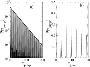
Figure 2: (a) Distribution function of time intervals between two consecutive quantum jumps for $\Delta=100$ $\tau_{0}=0.01$ and $10^{9}$ kicks; the solid line is a fit with $\tau_{d}=32$; (b) Enlargement of (a)

We assume that every “kick” provided by the function $\Delta(\tau)$ is followed by the collapse of the wave function. Before the kick, the spin points in (or opposite to) the direction of the effective magnetic field. After the kick there appears the finite angle $(\Delta\Theta)$ between the new direction of the effective field and the average spin. The probability for the spin to “accept” the “before-kick” direction relative to the new effective field is $\cos^{2}(\Delta\Theta/2)$. The probability to “accept” the opposite direction, i.e. the probability of a quantum jump is $\sin^{2}(\Delta\Theta/2)$. (It is clear that a significant probability of a quantum jump appears only when the effective field passes the transversal $x-y$-plane. In the transversal plane, the effective field has the minimum value. Thus, after every kick of the random field our computer code decides the “fate” of the spin in accordance with the probabilities of two events: to restore the previous direction relatively to the effective field, or to experience a quantum jump. In our model the CT experiences harmonic oscillations

$$x^{(\pm)}_{c}(\tau)=x_{m}\cos(1\pm\delta\omega)\tau,$$

where $(\pm)$ correspond to two CT trajectories with the spin pointing in the direction of (or opposite to) the corresponding effective field, and $\delta\omega$ is the CT frequency shift. The components of the effective field are given by

$$(\varepsilon,0,2\eta x_{c}(\tau)+\Delta(\tau)).$$

From the experimental data 1 for the CT amplitude $X_{m}=10$ nm we obtain $x_{m}=1.2\times 10^{5}$. The frequency shift, $\delta\omega$, can be estimated as 8

$$\delta\omega=\Delta\omega/\omega_{c}={{2G\mu_{B}}\over{\pi X_{m}k_{c}}}=4.2\times 10^{-7}.$$

Note that our model contains two important simplifications: first, we assume that the wave function collapse occurs immediately after the “kick” of the random field. Thus, we ignore the finite time when the spin-CT system is in an entangled state. Second, in a real situation the deviation of the spin from the effective field is a “quasi–resonance” process caused by the cantilever modes whose frequencies are close to the Rabi frequency. In our model this deviation appears as a result of the “kick” of the random field.

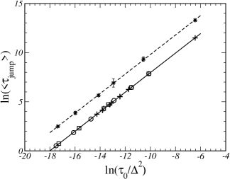
Figure 3: Dependence of the average time intervals between two consecutive quantum jumps on $\tau_{0}/\Delta^{2}$. The full line corresponds to the value $x_{m}=1.2\times 10^{-5}$, the squares represent $\delta\omega=4.2\times 10^{-8}$, the crosses $\delta\omega=4.2\times 10^{-7}$, the circles $\delta\omega=4.2\times 10^{-6}$ The dashed line corresponds to the value $x_{m}=7.2\times 10^{-5}$. Data have been obtained by varying parameters $\Delta$ and $\tau_{0}$ in the ranges: $10<\Delta<300$ and $0.001<\tau_{0}<1$.

Below we describe the results of our simulations. Fig. 2 demonstrates a typical probability distribution of time intervals, $\tau_{jump}$, between two consecutive quantum jumps. The probability distribution is a sequence of sharp peaks at $\tau_{jump}=\tau_{n}=n\pi$ with the Poisson-like amplitude

$$P(\tau_{n})\sim\exp(-\tau_{n}/\tau_{d}).$$

(Certainly, $P(\tau_{jump})=0$ at $\tau<\tau_{0}-\delta\tau$.) The sharp peak appears as the probability of the quantum jump is significant when the spin passes through the transversal plane, i.e. every half-period of the CT oscillation which is equal to $\pi$. The average value of the time interval $\langle\tau_{jump}\rangle$ was found to be

$$\langle\tau_{jump}\rangle\approx\tau_{d},$$

with an error less than 3%. The standard deviation is equal to $\tau_{d}$ with the same accuracy

$$(\langle\tau^{2}_{jump}\rangle-\langle\tau_{jump}\rangle^{2})^{1/2}\approx\tau_{d}.$$

We studied the dependence of the average value $\langle\tau_{jump}\rangle$ on the parameters of our model. We have found that $\langle\tau_{jump}\rangle$ does not depend on $\delta\tau$ or $\delta\omega$. (We varied $\delta\tau$ from $0$ to $\tau_{0}$ and changed $\delta\omega$ up to one order of magnitude.) At a fixed value of the amplitude $x_{m}$ the value of $\langle\tau_{jump}\rangle$ is approximately proportional to $\tau_{0}/\Delta^{2}$. Fig. 3 demonstrates this dependence.

The best fit for the numerical points in Fig. 3 is given by

$$\ln\langle\tau_{jump}\rangle=p+q\ln(\tau_{0}/\Delta^{2}).$$

For $x_{m}=1.2\times 10^{5}$ we have $p=17.9$, $q=0.993$. For the six fold value $x_{m}=7.2\times 10^{5}$ we obtained the same value of $q$ and $p=19.743$. If we estimate the amplitude of the random CT vibrations near the Rabi frequency as 1 pm, then $\Delta=1.8.$ Putting $\tau_{0}=\tau_{R}$ and the experimental value for $\tau_{R}$ (6) we obtain $\omega_{c}\langle\tau_{jump}\rangle=2.3$ s for $x_{m}=10nm$ and $\omega_{c}\langle\tau_{jump}\rangle=14.5$ s for $x_{m}=60nm$. These values are close to the experimental characteristic times of $3$ s and $20$ s reported in 1 .

Next we computed the correlation function for the CT frequency shift

$$C(\tau)={{\langle(\delta\omega(t)-\overline{\delta\omega})(\delta\omega(t+\tau)-\overline{\delta\omega})\rangle}\over{\langle(\delta\omega(t))^{2}\rangle-{\overline{\delta\omega}}^{2}}},$$

where $\overline{\delta\omega}=\langle\delta\omega(t)\rangle=0$, and $\langle...\rangle$ indicates an average over time.

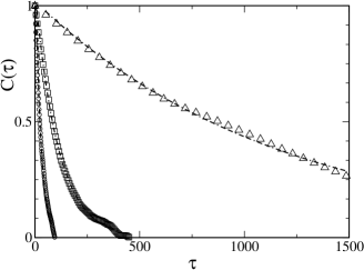
Figure 4: Correlation function of the CT frequency shift $C(\tau)$ for different parameters: circles $\Delta=100,\tau_{0}=10^{-2}$, squares $\Delta=50,\tau_{0}=10^{-2}$, triangles $\Delta=50,\tau_{0}=10^{-1}$. In all cases $\delta\tau=\tau_{0}/4$. The dashed curves show the exponential approximation of the correlation function $\exp(-\tau/\tau_{c})$ with $\tau_{c}=23.91,95.81,1179.15$, respectively.

In Fig.4 we show the correlation function $C(\tau)$ for three different values of parameters as indicated in the legend. As one can see, the general behavior is well described by the exponential function (indicated by dashed lines in Fig.4) $\exp(-\tau/\tau_{c})$. The relation between the correlation time $\tau_{c}$ and $\langle\tau_{jump}\rangle$ was found to be $\langle\tau_{jump}\rangle\simeq 2.5\tau_{c}$.

IV Conclusion

We developed a simple model which describes quantum jumps of spins in the OSCAR MRFM technique and which allowed us to compute the statistical characteristics of quantum jumps. In our model the average time interval $\langle\tau_{jump}\rangle$ between two consecutive jumps and the correlation time $\tau_{c}$ are proportional to the characteristic time of the magnetic noise, and inversely proportional to the square of the magnetic noise amplitude. Using experimental parameters 1 and a reasonable value for the CT noisy amplitude we obtained the value of $\langle\tau_{jump}\rangle$ which is close to the experimental value of the characteristic time of OSCAR MRFM signal.

References

- (1) H.J. Mamin, R. Budakian, B.W. Chui, D. Rugar, Phys. Rev. Lett. 91, 207604 (2003).
- (2) D. Mozyrsky, I. Martin, D. Pelekhov, P.C. Hammel, Appl. Phys. Lett. 82, 1278 (2003).
- (3) G.P. Berman, V.N. Gorshkov, D. Rugar, V.I. Tsifrinovich, Phys. Rev. B 68, 094402 (2003).
- (4) G.P. Berman, F. Borgonovi, G. Chapline, S.A. Gurvitz, P.C. Hammel, D.V. Pelekhov, A. Suter, V.I. Tsifrinovich, J. Phys. A: Math. Gen. 36, 4417 (2003).
- (5) G.P. Berman, F. Borgonovi, H.S. Goan, S.A. Gurvitz, V.I. Tsifrinovich, Phys. Rev. B 67, 094425 (2003).
- (6) G.P. Berman, F. Borgonovi, V.I. Tsifrinovich, quant-ph/0306107 (2003).
- (7) B.C. Stipe, H.J. Mamin, C.S. Yannoni, T.D. Stowe, T.W. Kenny, D. Rugar, Phys. Rev. Lett. 87, 277602 (2001).
- (8) G.P. Berman, D.I. Kamenev, V.I. Tsifrinovich, Phys. Rev. A 66, 023405 (2002).