Quasi dynamical symmetry in an interacting boson model phase transition

Abstract

The oft-observed persistence of symmetry properties in the face of strong symmetry-breaking interactions is examined in the SO(5)-invariant interacting boson model. This model exhibits a transition between two phases associated with U(5) and O(6) symmetries, respectively, as the value of a control parameter $\alpha$ progresses from 0 to 1. The remarkable fact is that, for intermediate values of $\alpha$ the model states exhibit the characteristics of its closest symmetry limit for all but a relatively narrow transition region that becomes progressively narrower as the particle number of the model increases. This phenomenon is explained in terms of quasi-dynamical symmetry.

There have been numerous recent studies of phase transitions in nuclear models PTs ; FI ; CZ ; Jolie ; LG . Being finite zero-temperature many-particle systems, nuclei do not exhibit the sharp phase transitions observed in condensed matter physics. Nevertheless, theoretical models designed to describe nuclei for particular values of their parameters can be extended to study their behavior as their parameters are varied, e.g. as the particle number goes to infinity.

This letter focuses on a phase transition FI in the interacting boson model (IBM) of Arima and Iachello AI . The IBM comprises $N$ boson particles each of which has two states: an $L=0$ ($s$-boson) state and an $L=2$ ($d$-boson) state with five orientations. The creation and annihilation operators for these bosons are denoted $\{s^{\dagger},d^{\dagger}_{\nu};\nu=0,\pm 1\pm 2\}$ and $\{s,d^{\nu};\nu=0,\pm 1\pm 2\}$, respectively. They satisfy the usual boson commutation relations

$$[s,s^{\dagger}]=1\,,\quad[d^{\mu},d^{\dagger}_{\nu}]=\delta_{\mu\nu}\,,[s,d^{\dagger}_{\nu}]=[d^{\nu},s^{\dagger}]=0\,.$$ (1)

Thus, the Hilbert space of the IBM carries an irreducible representation (irrep) of the group U(6) and can be realized as a subspace of states of $N$ quanta of a six-dimensional harmonic oscillator. The group U(6) has several subgroups and different phases of the model can be associated with Hamiltonians that are invariant under different subgroups. We consider the Hamiltonian AI ; FI

$$\hat{H}(\alpha)=(1-\alpha)\hat{H}_{1}+\alpha\hat{H}_{2}\,,$$ (2)

with control parameter $\alpha$, where $\hat{H}_{1}$ is the U(5)-invariant $d$-boson number operator and $\hat{H}_{2}$ is the O(6)-invariant operator:

$$\hat{H}_{1}=\hat{n}=\sum_{\nu}d^{\dagger}_{\nu}d^{\nu}\,,\quad\hat{H}_{2}=\frac{1}{N}\hat{S}_{+}\hat{S}_{-}\,,$$ (3)

where

$$\hat{S}_{+}=\textstyle{1\over 2}(d^{\dagger}\cdot d^{\dagger}-s^{\dagger}s^{\dagger}),\quad\hat{S}_{-}=\textstyle{1\over 2}(d\cdot d-ss)\,.$$ (4)

The electric quadrupole moment operator is represented in the model by

$$\hat{Q}_{\nu}=\frac{Z}{\sqrt{N}}(d^{\dagger}_{\nu}s+s^{\dagger}d_{\nu})\,,\quad\nu=0,\pm 1,\pm 2\,,$$ (5)

where $Z$ is a suitable norm factor (can be thought of as the charge).

This letter shows the behavior of the energy-level spectrum and the electric quadrupole transitions for the above model as $\alpha$ is varied over the range $0\leq\alpha\leq 1$. The model is analytically solvable in its U(5) $(\alpha=0)$ and O(6) $(\alpha=1)$ symmetry limits. The numerically computed results given below for $0\leq\alpha\leq 1$ are determined by use of the simple ${\rm SU}(1,1)^{s}\times{\rm SU}(1,1)^{d}$ spectrum generating algebra with basis elements

$$\begin{array}[]{c}\hat{S}^{s}_{+}=\textstyle{1\over 2}s^{\dagger}s^{\dagger},\quad\hat{S}^{s}_{-}={1\over 2}ss,\\ \hat{S}^{s}_{0}=\textstyle{1\over 4}(s^{\dagger}s+ss^{\dagger})\,,\end{array}$$ (8)

$$\begin{array}[]{c}\hat{S}^{d}_{+}=\textstyle{1\over 2}d^{\dagger}\cdot d^{\dagger},\quad\hat{S}^{d}_{-}={1\over 2}d\cdot d,\\ \hat{S}^{d}_{0}=\textstyle{1\over 4}(d^{\dagger}\cdot d+d\cdot d^{\dagger})\,.\end{array}$$ (11)

Energy levels, labelled by an SO(5) quantum number $v$, and E2 transition rates for decay of the first excited state of the model are shown as a function of $\alpha$ in figs. 1-2.

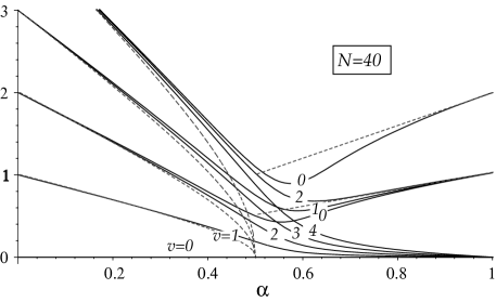
Figure 1: Excitation energies of the Hamiltonian $\hat{H}(\alpha)$ plotted as a function of $\alpha$. Precise, numerically computed, energies are shown as continuous lines. The dotted lines are the results of an RPA calculation (for $\alpha<0.5$) and of another harmonic aproximation (for $\alpha>0.5$).

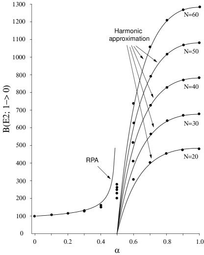
Figure 2: $B$(E2) transition rates for decay of the first excited $v=1$ energy level to the ground state in the IBM for various values of $N$ expressed in units such that $B({\rm E}2;1\to 0)=100$ in the U(5) $(\alpha=0)$ limit. The continuous lines for $\alpha\leq 0.5$ are for the RPA and those for $\alpha\geq 0$ are for the harmonic approximation.

A superficial look at the results of figs. 1 and 2 would seem to suggest that the model holds onto its U(5) symmetry for $0\leq\alpha\lesssim 0.3$ and to its O(6) symmetry for $0.8\gtrsim\alpha\leq 1$ and that there is a transition between the states of one symmetry to the other in the intermediate region. It turns out this is an overly simplistic view of what happens. Insight into the actual evolution of the model states with increasing $\alpha$ is given by approximate solutions which predict a phase transition and do so with increasing accuracy as $N$ increases. We consider the familiar Random Phase Approximation for $0\leq\alpha\leq 0.5$ and another harmonic approximation for $0.5\leq\alpha\leq 1$.

For small values of $\alpha$, the RPA gives quasi-boson excitation operators

$$D^{\dagger}_{\nu}=(x\,d^{\dagger}_{\nu}s-y\,s^{\dagger}d_{\nu})/\sqrt{N}\,,$$ (12)

with coefficients that satisfy an eigenvector equation of the non-Hermitean form

$$\left(\begin{array}[]{cc}A&B\\ -B&-A\end{array}\right)\left(\begin{array}[]{cc}x\\ y\end{array}\right)=\varepsilon\left(\begin{array}[]{cc}x\\ y\end{array}\right)\,,$$ (13)

with submatrices given, e.g. in the double-commutator equations of motion formalism EoM , by

$$A_{\mu\nu}={1\over N}\langle\phi|[s^{\dagger}d^{\mu},[H(\alpha),d^{\dagger}_{\nu}s]]|\phi\rangle=\Big{(}1-{3\over 2}\alpha\Big{)}\delta_{\mu\nu}\,,\quad$$ (14)

$$B_{\mu\nu}={-1\over N}\langle\phi|[s^{\dagger}d^{\mu},[H(\alpha),s^{\dagger}d_{\nu}]]|\phi\rangle=-{1\over 2}\alpha\delta_{\mu\nu}\,,$$ (15)

where $|\phi\rangle$ is the uncorrelated ground state given by the $s$-boson condensate $|\phi\rangle=(s^{\dagger})^{N}|0\rangle/\sqrt{N!}$. The RPA energy spectrum is shown in fig. 1 as dotted lines for $\alpha\leq 0.5$. It predicts a collapse of the excitation energies to zero and, in fig. 2, a divergence of the E2 transition rate for decay of the $v=1$ first excited state as $\alpha\to 0.5$. Thus, the RPA predicts a phase transition at $\alpha_{\rm crit}=0.5$ in accord with Thouless’ Hartree-Fock stability condition Thouless .

Details of the calculations will be given in an article to follow. It will then also be shown that there is another harmonic approximation complementary to the RPA which gives the spectrum accurately in the $\alpha\lesssim 1$ region. The essential ingredients of this approximation are shown in fig. 3

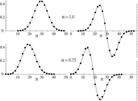
Figure 3: Wave functions for the $N=60$ ground state and first excited $v=0$ state for $\alpha=1$ and $0.75$. The dots give the coefficients of the states in a basis of $d$-boson number $n$. The continuous lines are those of the harmonic approximation.

which gives the expansion coefficients of the lowest and first excited $v=0$ states for $\alpha=1.0$ and 0.75 (cf. states labelled by $v$ in fig. 1) in a basis $\{|nv\!=\!0\rangle\}$ which diagonalizes the Hamiltonian $\hat{H}_{1}$ ($n$ is the $d$-boson number). The smooth curves through these numerically computed coefficients are simply harmonic oscillator wave functions centred about $N/2$ for $\alpha=1$ and shifted to smaller mean values of $n$, in the manner of coherent state wave functions, as $\alpha$ is decreased. The energy levels and E2 transition rates predicted by this approximation are shown for $0.5\leq\alpha\leq 1$ in figs. 1-2. They are precise for $\alpha=1$ and become increasingly accurate for smaller $\alpha$ with increasing values of the boson number $N$.

An examination of the physical significance of the wave functions of fig. 3 reveals that they represent a nucleus with a large mean quadrupole deformation at $\alpha=1$ that decreases as $\alpha$ falls and the nucleus moves towards a spherical equilibrium shape. Such behavior is expected from the form of the classical potential energy Diep corresponding to the Hamiltonian (2). This potential, given as a function

$$V_{\alpha}(\beta)=N\big{[}\beta^{2}+\alpha(-2\beta^{2}+\beta^{4})+0(\frac{1}{N})\big{]}$$ (16)

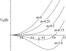
Figure 4: The classical potential energy $V_{\alpha}(\beta)$ for different values of $\alpha$.

of $\alpha$ and a classical quadrupole shape variable $\beta$, is shown for a few values of $\alpha$ in fig. 4. The magnitude of the E2 (electric quadrupole) gamma-ray transition rate shown in fig. 2 is closely related to the mean square quadrupole moment of the ground state and a good indicator of how the mean value of the quadrupole moment actually evolves with $\alpha$ in the model.

Figure 3 reveals that the eigenfunctions of $\hat{H}(\alpha)$ for $0.75\lesssim\alpha\leq 1$ are close approximations to harmonic oscillator (Glauber) coherent state wave functions. However, as $\alpha$ falls below 0.75 (for $N=60$), the wave functions reach the lower $n=0$ boundary and the harmonic approximation begins to break down. For larger values of $N$, when the potential $V_{\alpha}$ becomes deeper and the widths of the harmonic oscillator wave functions narrower, the approximation holds for smaller values of $\alpha$. However, at $\alpha=0.5$, the centroid of the wave functions of the harmonic approximation lie precisely at $n=0$; thus the model breaks down as $\alpha\to 0.5$ for all values of $N$. This is what one would expect for the quantum states of a model with potential energy given by eqn. (16).

Similar insights can be gained for small $\alpha$ from the RPA. For large values of $N$, in which the RPA is equivalent to the Bogolyubov approximation of replacing the $s$-boson operators $s^{\dagger}$ and $s$ by the c-number $\sqrt{N}$, the RPA transformation of eqn. (12) is seen as an SU(1,1) transformation

$$d^{\dagger}_{\nu}\to D^{\dagger}_{\nu}=x\,d^{\dagger}_{\nu}-y\,d_{\nu}\,.$$ (17)

The corresponding transformation of the ground state (to a $D$-boson vacuum) is then a transformation to a dilated (anti-squeezed) coherent state in which the equilibrium quadrupole shape remains spherical but the width of its (harmonic oscillator Gaussian) wave function, along with the magnitude of the quadrupole shape fluctuations grow with increasing $\alpha$. As $\alpha$ approaches the critical value 0.5 from below, the spherical equibrium shape, indicated by the potential shown in fig. 4, becomes unstable and the width of the $D$-boson vacuum wave function diverges.

The precision of the RPA and the other harmonic approximation, for low-energy model states outside of a transition region that becomes increasingly narrow as $N\to\infty$, suggests a useful definition of the concept of phase in such situations.

Definition (phase): If SGC is a subgroup chain

$$G_{1}\supset G_{2}\subset\cdots$$ (18)

of transformations of a system, then a subset of states of the system is said to be in an SGC-phase if the properties of the subset are indistinguishable (to within a specified accuracy) from a corresponding subset of states of a model whose eigenstates belong to irreps of the subgroups in the chain and whose observables are infinitesimal generators of $G_{1}$.

The above results show that there is domain of $\alpha$ extending from 0 to some upper limit below 0.5 for which a subset of low-energy states are described accurately by the RPA. The RPA formalism shows that these states are equivalently described by a U(5)-invariant model Hamiltonian

$$\hat{H}_{\rm RPA}=\varepsilon\sum_{\nu}D^{\dagger}_{\nu}D^{\nu}+{\rm constant}\,,$$ (19)

with electric quadrupole operator

$$\hat{Q}^{\rm RPA}_{\nu}=\frac{Z}{\sqrt{N}}(D^{\dagger}_{\nu}s+s^{\dagger}D_{\nu})\,,\quad\nu=0,\pm 1,\pm 2\,.$$ (20)

Thus, according to the definition, the subspace of states that are described to within the required limits of accuracy by the RPA, for a given value of $\alpha$, belong to a ${\rm U(6)}\supset{\rm U(5)}\supset{\rm SO(5)}$ phase.

It is similarly shown that the subset of states whose energies cluster around those of the harmonic approximation for $\alpha\lesssim 1$ span an O(6) irrep (for some choice of O(6)). Moreover, to the extent that the harmonic approximation gives an accurate description of a subset of states in this region, the energy levels and E2 transitions between these states are accurately described by a model whose states are labelled by the quantum numbers of a ${\rm U(6)}\supset{\rm O(6)}\supset{\rm SO(5)}$ subgroup chain (the small spread of energies of a cluster is readily accommodated by including a term proportional to the ${\rm SO(5)}\subset{\rm O(6)}$ Casimir invariant in model Hamiltonian). Thus, by the definition, the states that are accurately described by the harmonic approximation, belong to a ${\rm U(6)}\supset{\rm O(6)}\supset{\rm SO(5)}$ phase.

The above analysis of the nature of the solutions of the IBM Hamiltonian (2) in terms of the RPA shows why, in spite of the fact that the U(5) symmetry of $\hat{H}(0)=\hat{H}_{1}$ is quickly broken by the $\alpha\hat{H}_{2}$ term in $\hat{H}(\alpha)$ for $\alpha>0$, the results look as though the U(5) symmetry is preserved. Similarly, the harmonic approximation of $0.5\gtrsim\alpha\leq 1$ shows why the apparent O(6) symmetry is also retained over a considerably larger region of $\alpha$ than expected.

An apparent persistence of a symmetry when numerical calculations show there to be strong mixing of the irreps of the symmetry group in question has been observed many times. It has been expressed in terms of what has been dubbed quasi-dynamical symmetry QDS1 ; cf. ref. QDS2 for a review.

A sense of what quasi-dynamical symmetry means is obtained by recalling that different but equivalent irreps of a group can be combined coherently to give new (equivalent) irreps. A simple example would be the coherent mixing of the basis states $\{|aLM\rangle\}$ and $\{|bLM\rangle\}$ of two irreps of SO(3) of angular momentum L to form new basis states

$$|cLM\rangle=C_{a}|aLM\rangle+C_{b}|bLM\rangle$$ (21)

for an equivalent mixed irrep of the same $L$; coherent mixing means that the coefficients $C_{a}$ and $C_{b}$ are independent of $M$. Quasi-dynamical symmetry arises because many groups have distinct irreps that are similar and difficult to distinguish, especially by consideration of a subset of their states. Thus, for example, it is possible to represent many states of a free particle with wave functions of good linear momentum even though the real states are wave packets comprising coherent mixtures of plane wave functions of similar momentum.

It is not surprising then to find that subsets of states of a given system can be described by models with dynamical symmetries that are only quasi-dynamical symmetries of the sytem being described. Because a model can at best describe a subset of the states of a real physical system to within limited accuracy, it could not be otherwise. However, an explicit recognition of the possible quasi-dynamical symmetries of physical systems is invaluable for interpreting the implications of successful models and in designing successful approximations. In this note, I have explicitly determined realizations of the quasi-dynamical symmetries of two phases of the IBM and thereby obtained an explanation of why these symmetries appear to persist in spite of the known presence of strong symmetry mixing interactions. Simply stated, the mixed states of the original dynamical group become the unmixed states of a quasi-dynamical group.

The above perspective leads one to think of the evolution of the low-energy states of the IBM as they progress though a phase transition in terms of the evolution of the quasi-dynamical group. In approximate pictorial terms, the effect of the symmetry-breaking interaction is primarily to distort the quasi-dynamical symmetry, rather than break it until a critical point is reached at which it can be distorted no more. At this point the symmetry really starts to break up; the system enters the transition region and, as it emerges on the other side, a new quasi-dynamical symmetry associated with another other phase begins to develop.

An interesting characteristic of the above results is that for reasonably large values of the boson number $N$, the low-energy states of the model can be assigned to one of three domains: one for which the ${\rm U(6)}\supset{\rm U(5)}\supset{\rm SO(5)}$ phase is appropriate, one for which the ${\rm U(6)}\supset{\rm O(6)}\supset{\rm SO(5)}$ phase is appropriate, and an intermediate transition domain which shrinks with increasing $N$. A recent suggestion of critical point symmetries FI which apply in the middle of the transition region is therefore of considerable interest; for example, it suggests that it might be meaningful to think of an intermediate phase separating the other two. This suggests that an interesting sequel to the present investigation would be an exploration of the ways the properties of the system in the transition domain evolve as a function of the boson number $N$.

- (1) H. Chen, J Brownstein and D.J Rowe, Phys. Rev. C42 1422 (1990); H. Chen, T. Song and D.J. Rowe, , Nucl. Phys. A582 181 (1995); D.J. Rowe, C. Bahri and W. Wijesundera, Phys. Rev. Lett. 80 (1998) 4394; C. Bahri, D.J. Rowe, and W. Wijesundera, Phys. Rev. C 58, 1539 (1998).
- (2) R.F. Casten and N.V. Zamfir, Phys. Rev. Lett. 85, 3584 (2000).
- (3) F. Iachello, Phys. Rev. Lett. 85, 3580 (2000); 87, 052502 (2001); 91, 132502 (2003).
- (4) J. Jolie, et al., Phys. Rev. Lett. 89, 182502 (2002).
- (5) A. Leviatan and J.N. Ginocchio, Phys. Rev. Lett. 90, 212501 (2003).
- (6) A. Arima and F. Iachello, Ann. Phys. 99, 253 (1976); 111, 201 (1978); O. Scholten, A. Arima and F. Iachello, Ann. Phys. 115, 325 (1978); F. Iachello and A. Arima, The Interacting Boson Model (Cambridge, 1987).
- (7) D.J. Rowe, Rev. Mod. Phys. 40, 153 (1968).
- (8) D.J. Thouless, Nucl. Phys. 21, 225 (1960).
- (9) A.E.L. Dieperink, O. Scholten, and F. Iachello, Phys. Rev. Lett. 44, 1747 (1980).
- (10) J. Carvalho, R. Le Blanc, M. Vassanji, D.J. Rowe and J. McGrory, 1986, Nucl. Phys. A452, 240 (1986); D.J. Rowe, P. Rochford and J. Repka, J. Math. Phys. 29, 572 (1988); P. Rochford and D.J. Rowe, Phys. Lett. B210, 5 (1988).
- (11) D.J. Rowe, “Embedded representations and quasi-dynamical symmetry” in ‘Computational and Group Theoretical Methods in Nuclear Physics Proc. Symp. in Honor of Jerry P. Draayer’s 60th Birthday, Playa del Carmen, Mexico, 18-21 February 2003 (Eds. O. Castańos, J. Escher, J. Hirsch, S. Pittel, and G. Stoicheva. World Scientific, Singapore, in press).