The $\mathcal{C}$ Operator in $\mathcal{PT}$-Symmetric
Quantum Theories

Abstract

The Hamiltonian $H$ specifies the energy levels and the time evolution of a quantum theory. It is an axiom of quantum mechanics that $H$ be Hermitian because Hermiticity guarantees that the energy spectrum is real and that the time evolution is unitary (probability preserving). This paper investigates an alternative way to construct quantum theories in which the conventional requirement of Hermiticity (combined transpose and complex conjugate) is replaced by the more physically transparent condition of space-time reflection ($\mathcal{PT}$) symmetry. It is shown that if the $\mathcal{PT}$ symmetry of a Hamiltonian $H$ is not broken, then the spectrum of $H$ is real. Examples of $\mathcal{PT}$-symmetric non-Hermitian quantum-mechanical Hamiltonians are $H=p^{2}+ix^{3}$ and $H=p^{2}-x^{4}$. The crucial question is whether $\mathcal{PT}$-symmetric Hamiltonians specify physically acceptable quantum theories in which the norms of states are positive and the time evolution is unitary. The answer is that a Hamiltonian that has an unbroken $\mathcal{PT}$ symmetry also possesses a physical symmetry represented by a linear operator called $\mathcal{C}$. Using $\mathcal{C}$ it is shown how to construct an inner product whose associated norm is positive definite. The result is a new class of fully consistent complex quantum theories. Observables are defined, probabilities are positive, and the dynamics is governed by unitary time evolution. After a review of $\mathcal{PT}$-symmetric quantum mechanics, new results are presented here in which the $\mathcal{C}$ operator is calculated perturbatively in quantum mechanical theories having several degrees of freedom.

1 Introduction

In this paper we present a brief review of some recent work on an alternative way to formulate of quantum mechanical models and present new results concerning the perturbative calculation of what has become known in this theory as the $\mathcal{C}$ operator.

In the conventional formulation of quantum mechanics the Hamiltonian $H$, which incorporates the symmetries and specifies the dynamics of a quantum theory, must be Hermitian: $H=H^{\dagger}$. The usual meaning of the symbol $\dagger$, which indicates Dirac Hermitian conjugation, is combined transpose and complex conjugation. It is commonly thought that a Hamiltonian must be Hermitian in order to ensure that the energy spectrum (the eigenvalues of $H$) is real and that the time evolution of the theory is unitary (probability is conserved in time). Although $H=H^{\dagger}$ is sufficient to guarantee these properties, it is not necessary. Indeed, we believe that this condition of Hermiticity is a mathematical requirement whose physical basis is somewhat obscure. Recently, a more physical alternative axiom called space-time reflection symmetry ($\mathcal{PT}$ symmetry), $H=H^{\mathcal{PT}}$, has been investigated. This symmetry allows for the possibility of complex non-Hermitian Hamiltonians but still leads to a consistent theory of quantum mechanics.

Because $\mathcal{PT}$ symmetry is an alternative condition to conventional Hermiticity, it is now possible to construct infinitely many new Hamiltonians that would have been rejected in the past because they are not Hermitian in the usual sense. One example of such a Hamiltonian is $H=\mbox{$\textstyle\frac{1}{2}$}p^{2}+\mbox{$\textstyle\frac{1}{2}$}\mu^{2}x^{2}+i\epsilon x^{3}$, which is the quantum mechanical analog of the quantum field theoretic Hamiltonian $H=\int d{\bf x}\left[\mbox{$\textstyle\frac{1}{2}$}\pi^{2}+\mbox{$\textstyle\frac{1}{2}$}(\nabla\varphi)^{2}+\mbox{$\textstyle\frac{1}{2}$}\mu^{2}\varphi^{2}+i\epsilon\varphi^{3}\right]$. Another example of a $\mathcal{PT}$-symmetric non-Hermitian Hamiltonian is $H=\mbox{$\textstyle\frac{1}{2}$}p^{2}+\mbox{$\textstyle\frac{1}{2}$}\mu^{2}x^{2}-\epsilon x^{4}$, which is the $\mathcal{PT}$-symmetric analog of the quantum field theoretic Hamiltonian $H=\int d{\bf x}\left[\mbox{$\textstyle\frac{1}{2}$}\pi^{2}+\mbox{$\textstyle\frac{1}{2}$}(\nabla\varphi)^{2}+\mbox{$\textstyle\frac{1}{2}$}\mu^{2}\varphi^{2}-\epsilon\varphi^{4}\right]$. This latter Hamiltonian could be an interesting candidate for describing the Higgs sector of the standard model. It should be emphasized that we do not regard the condition of conventional Hermiticity as wrong. Rather, we view the condition of $\mathcal{PT}$ symmetry as offering the possibility of studying new kinds of quantum theories that have heretofore never been studied because they have been thought to be physically unacceptable.

Let us review the properties of the space reflection (parity) operator $\mathcal{P}$ and the time-reflection operator $\mathcal{T}$: $\mathcal{P}$ is a linear operator with the property that $\mathcal{P}^{2}=1$ and has the effect $p\to-p$ and $x\to-x$; $\mathcal{T}$ is an antilinear operator with the property that $\mathcal{T}^{2}=1$ and has the effect $p\to-p$, $x\to x$, and $i\to-i$. The operator $\mathcal{T}$ is called antilinear because it changes the sign of $i$. We know that it reverses the sign of $i$ because, like $\mathcal{P}$, this operator preserves the fundamental commutation relation of quantum mechanics, $[x,p]=i$, known as the Heisenberg algebra.

It is easy to construct Hamiltonians of the form $H=p^{2}+V(x)$ that are not Hermitian but do possess $\mathcal{PT}$ symmetry. The trick is to take the potential to be a function of $ix$: $V=V(ix)$. We also impose a general condition that has not been widely emphasized in the literature; namely, we require that $H$ be symmetric: $H=H^{\rm T}$, where ${\rm T}$ represents the transpose. The reason for this symmetry condition will become clear later on. For example, consider the one-parameter family of symmetric Hamiltonians

$$H=p^{2}+x^{2}(ix)^{\epsilon},$$ (1)

where $\epsilon$ is real. While $H$ in (1) is not symmetric under $\mathcal{P}$ or $\mathcal{T}$ separately, it is invariant under their combined operation. Such Hamiltonians are said to possess space-time reflection symmetry. Other examples of complex Hamiltonians having $\mathcal{PT}$ symmetry are $H=p^{2}+x^{4}(ix)^{\epsilon}$, $H=p^{2}+x^{6}(ix)^{\epsilon}$, and so on [1]. Note that these classes of Hamiltonians are all different. For example, the Hamiltonian obtained by continuing $H$ in (1) along the path $\epsilon:\,0\to 8$ has a different spectrum from the Hamiltonian that is obtained by continuing $H=p^{2}+x^{6}(ix)^{\epsilon}$ along the path $\epsilon:\,0\to 4$. This is because the boundary conditions on the eigenfunctions are different.

The class of $\mathcal{PT}$-symmetric Hamiltonians is larger than and includes real symmetric Hermitians because any real symmetric Hamiltonian is $\mathcal{PT}$-symmetric. For example, consider the real symmetric Hamiltonian $H=p^{2}+x^{2}+2x$. This Hamiltonian is time-reversal symmetric, but according to the usual definition of space reflection for which $x\to-x$, this Hamiltonian does not appear to have $\mathcal{PT}$ symmetry. However, the parity operator is defined only up to unitary equivalence, and if we express the Hamiltonian in the form $H=p^{2}+(x+1)^{2}-1$, then it is evident that $H$ is $\mathcal{PT}$ symmetric provided that the parity operator performs a space reflection about the point $x=-1$ rather than $x=0$. See Ref. [2] for the general construction of the relevant parity operator.

With properly defined boundary conditions the spectrum of the Hamiltonian $H$ in (1) is real and positive when $\epsilon\geq 0$ [3] and the spectrum is partly real and partly complex when $\epsilon<0$. The eigenvalues have been computed numerically to very high precision, and the real eigenvalues are plotted as functions of $\epsilon$ in Fig. 1.

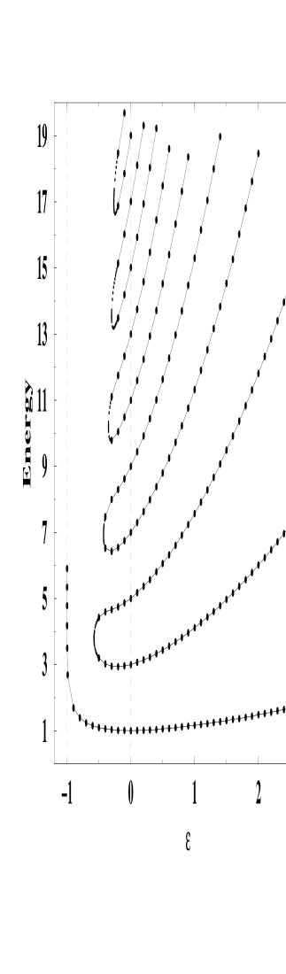
Figure 1: Energy levels of the Hamiltonian $H=p^{2}+x^{2}(ix)^{\epsilon}$ as a function of the parameter $\epsilon$. There are three regions: When $\epsilon\geq 0$, the spectrum is real and positive and the energy levels rise with increasing $\epsilon$. The lower bound of this region, $\epsilon=0$, corresponds to the harmonic oscillator, whose energy levels are $E_{n}=2n+1$. When $-1<\epsilon<0$, there are a finite number of real positive eigenvalues and an infinite number of complex conjugate pairs of eigenvalues. As $\epsilon$ decreases from $0$ to $-1$, the number of real eigenvalues decreases; when $\epsilon\leq-0.57793$, the only real eigenvalue is the ground-state energy. As $\epsilon$ approaches $-1^{+}$, the ground-state energy becomes infinite. When $\epsilon\leq-1$ there are no real eigenvalues.

The $\mathcal{PT}$ symmetry of a Hamiltonian $H$ is said to be unbroken if all of the eigenfunctions of $H$ are simultaneously eigenfunctions of $\mathcal{PT}$. Note that even if a system is defined by an equation that possesses a discrete symmetry, the solution to this equation need not exhibit that symmetry. For example, although the differential equation ${\ddot{y}}(t)=y(t)$ is symmetric under time reversal $t\to-t$, the solutions $y(t)=e^{t}$ and $y(t)=e^{-t}$ do not exhibit time-reversal symmetry; other solutions, such as $y(t)=\cosh(t)$, are time-reversal symmetric. The same is true of a system whose Hamiltonian is $\mathcal{PT}$ symmetric. Even if the Schrödinger equation and corresponding boundary conditions are $\mathcal{PT}$ symmetric, the wave function that solves the Schrödinger equation boundary value problem need not be symmetric under space-time reflection. When the solution exhibits $\mathcal{PT}$ symmetry, we say that the $\mathcal{PT}$ symmetry is unbroken. Conversely, if the solution does not possess $\mathcal{PT}$ symmetry, we say that the $\mathcal{PT}$ symmetry is broken.

It is extremely easy to prove that if the $\mathcal{PT}$ symmetry of a Hamiltonian $H$ is unbroken, then the spectrum of $H$ is real: Assume that (i) $H$ possesses $\mathcal{PT}$ symmetry (that is, that $H$ commutes with the $\mathcal{PT}$ operator), and (ii) if $\phi$ is an eigenstate of $H$ with eigenvalue $E$, then it is simultaneously an eigenstate of $\mathcal{PT}$ with eigenvalue $\lambda$ (it is this second assumption of unbroken $\mathcal{PT}$ symmetry that is crucial):

$$H\phi=E\phi\quad{\rm and}\quad\mathcal{PT}\phi=\lambda\phi.$$ (2)

We first show that the eigenvalue $\lambda$ is a pure phase. We multiply $\mathcal{PT}\phi=\lambda\phi$ on the left by $\mathcal{PT}$ and use the fact that $\mathcal{P}$ and $\mathcal{T}$ commute and that $\mathcal{P}^{2}=\mathcal{T}^{2}=1$ to conclude that $\phi=\lambda^{*}\lambda\phi$ and thus $\lambda=e^{i\alpha}$ for some real $\alpha$. Next, we introduce a convention used throughout this paper. Without loss of generality we replace the eigenstate $\phi$ by $e^{-i\alpha/2}\phi$ so that its eigenvalue under the operator $\mathcal{PT}$ is unity: $\mathcal{PT}\phi=\phi$. Next, we multiply the eigenvalue equation $H\phi=E\phi$ on the left by $\mathcal{PT}$ and use $[\mathcal{PT},H]=0$ to obtain $E\phi=E^{*}\phi$. Hence, $E=E^{*}$ and the eigenvalue $E$ is real.

The crucial step in the argument above is the assumption that $\phi$ is simultaneously an eigenstate of $H$ and $\mathcal{PT}$. In quantum mechanics if a linear operator $X$ commutes with the Hamiltonian $H$, then the eigenstates of $H$ are also eigenstates of $X$. However, we emphasize that the operator $\mathcal{PT}$ is not linear (it is antilinear) and thus we must make the extra assumption that the $\mathcal{PT}$ symmetry of $H$ is unbroken; that is, that $\phi$ is simultaneously an eigenstate of $H$ and $\mathcal{PT}$. This extra assumption is nontrivial because it is difficult to determine a priori whether the $\mathcal{PT}$ symmetry of a particular Hamiltonian $H$ is broken or unbroken. For the Hamiltonian $H$ in (1) the $\mathcal{PT}$ symmetry is unbroken when $\epsilon\geq 0$ and it is broken when $\epsilon<0$. The conventional Hermitian Hamiltonian for the quantum mechanical harmonic oscillator lies at the boundary of the unbroken and the broken regimes. Recently, Dorey et al. proved rigorously that the spectrum of $H$ in (1) is real and positive [4] in the region $\epsilon\geq 0$. Many other $\mathcal{PT}$-symmetric Hamiltonians for which space-time reflection symmetry is not broken have been investigated, and the spectra of these Hamiltonians have also been shown to be real and positive [5].

It is important to know whether a given non-Hermitian $\mathcal{PT}$-symmetric Hamiltonian has a positive real spectrum, but the most urgent question is whether such a Hamiltonian defines a physical theory of quantum mechanics. By a physical theory we mean that there is a Hilbert space of state vectors and that this Hilbert space has an inner product with a positive norm. In quantum mechanics we interpret the norm of a state as a probability and this probability must be positive. Furthermore, we must show that the time evolution of the theory is unitary. This means that as a state vector evolves in time the probability does not leak away. With these considerations in mind one would wonder whether a Hamiltonian such as $H$ in (1) gives a consistent quantum theory. Indeed, early investigations of this Hamiltonian have shown that while the spectrum is entirely real and positive when $\epsilon\geq 0$, one inevitably encountered the severe problem of a Hilbert space endowed with an indefinite metric [6].

However, there is a new symmetry that all $\mathcal{PT}$-symmetric Hamiltonians having an unbroken $\mathcal{PT}$-symmetry possess [7]. We denote the operator representing this symmetry by $\mathcal{C}$ because the properties of this operator resemble those of the charge conjugation operator in particle physics. This allows us to introduce an inner product structure associated with $\mathcal{CPT}$ conjugation for which the norms of quantum states are positive definite. Because of this we can say that $\mathcal{PT}$ symmetry is an alternative to conventional Hermiticity; it introduces the new concept of a dynamically determined inner product (one that is defined by the Hamiltonian itself). Consequently, we can extend the Hamiltonian and its eigenstates into the complex domain so that the associated eigenvalues are real and the underlying dynamics is unitary. This shows that $\mathcal{PT}$-symmetric Hamiltonians are Hermitian in an extended (non-Dirac) sense.

This paper is organized as follows. In Sec. 2 we give a general discussion of the $\mathcal{C}$ operator and in Sec. 3 we present a simple $2\times 2$ matrix example of this operator. In Sec. 4 we show how to calculate $\mathcal{C}$ using perturbation theory for the cubic Hamiltonian $H=\mbox{$\textstyle\frac{1}{2}$}p^{2}+\mbox{$\textstyle\frac{1}{2}$}\mu^{2}x^{2}+i\epsilon x^{3}$. In Secs. 5 and 6 we calculate $\mathcal{C}$ for quantum mechanical Hamiltonians having two and three degrees of freedom. This is the principal new result in this paper. In Secs. 7 and 8 we consider possible physical applications and draw some conclusions.

2 Construction of the $\mathcal{C}$ Operator

We begin by summarizing the mathematical properties of the solution to the Sturm-Liouville differential equation eigenvalue problem

$$-\phi_{n}^{\prime\prime}(x)+x^{2}(ix)^{\epsilon}\phi_{n}(x)=E_{n}\phi_{n}(x)$$ (3)

associated with the Hamiltonian $H$ in (1). This differential equation must be imposed on an infinite contour in the complex-$x$ plane. For large $|x|$ this contour lies in wedges placed symmetrically with respect to the imaginary-$x$ axis [3]. The boundary conditions on the eigenfunctions are that $\phi(x)\to 0$ exponentially rapidly as $|x|\to\infty$ along the contour. For $0\leq\epsilon<2$, the contour may lie on the real axis.

When $\epsilon\geq 0$, the Hamiltonian has an unbroken $\mathcal{PT}$ symmetry. Thus, we know that the eigenfunctions $\phi_{n}(x)$ are simultaneously eigenstates of the $\mathcal{PT}$ operator:

$$\mathcal{PT}\phi_{n}(x)=\lambda_{n}\phi_{n}(x).$$ (4)

As we argued above, $\lambda_{n}$ is a pure phase and, without loss of generality, for each $n$ this phase can be absorbed into $\phi_{n}(x)$ by a multiplicative rescaling so that the new eigenvalue under $\mathcal{PT}$ is unity:

$$\mathcal{PT}\phi_{n}(x)=\phi_{n}^{*}(-x)=\phi_{n}(x).$$ (5)

It is not known rigorously yet, but there is strong evidence that when properly normalized the eigenfunctions $\phi_{n}(x)$ are complete. The coordinate-space statement of completeness reads

$$\sum_{n}(-1)^{n}\phi_{n}(x)\phi_{n}(y)=\delta(x-y)\qquad(x,y~{}{\rm real}).$$ (6)

This nontrivial result has been verified numerically to extremely high accuracy (twenty decimal places) [8, 9]. There is a factor of $(-1)^{n}$ in the sum. This unusual factor does not appear in conventional quantum mechanics. The presence of this factor is explained in the following discussion of orthonormality [see (8)] in which we encounter the problem associated with non-Hermitian $\mathcal{PT}$-symmetric Hamiltonians.

There seems to be a natural choice for the inner product of two functions $f(x)$ and $g(x)$:

$$(f,g)\equiv\int dx\,[\mathcal{PT}f(x)]g(x),$$ (7)

where $\mathcal{PT}f(x)=[f(-x)]^{*}$ and the integration path is the appropriate contour in the complex-$x$ plane. [We will see that (7) is not the correct choice for an inner product because it gives an indefinite metric. The correct inner product will be defined shortly, but studying this inner product is useful because it reveals the underlying mathematical structure of the theory.] The apparent advantage of this inner product is that the associated norm $(f,f)$ is independent of the overall phase of $f(x)$ and is conserved in time because $H$ commutes with $\mathcal{PT}$ and the time-evolution operator is $e^{-iHt}$. Phase independence is desired because in quantum mechanics the objective is to construct a space of rays to represent quantum mechanical states. With respect to this inner product, the eigenfunctions $\phi_{m}(x)$ and $\phi_{n}(x)$ of $H$ in (1) are orthogonal for $n\neq m$ because $H$ is symmetric. However, when we set $m=n$ we see by direct numerical calculation that the norm is evidently not positive:

$$(\phi_{m},\phi_{n})=(-1)^{n}\delta_{mn}.$$ (8)

This result is apparently true for all values of $\epsilon$ in (3), and it has been verified numerically to extremely high precision. Because the norms of the eigenfunctions alternate in sign, the metric associated with the $\mathcal{PT}$ inner product $(\cdot,\cdot)$ is indefinite. This sign alternation appears to be a generic feature of this $\mathcal{PT}$ inner product. [Extensive numerical calculations verify that the formula in (8) holds for all $\epsilon\geq 0$.] We emphasize that while the sign of the norm of $\phi_{n}$ is hard to verify analytically, the orthogonality of $\phi_{m}$ and $\phi_{n}$ is a trivial consequence of the symmetry of $H$. It is necessary to assume that $H$ be symmetric in order to have this orthogonality.

In spite of the nonpositivity of the inner product, it is instructive to proceed with the usual analysis that one would perform for any Sturm-Liouville problem of the form $H\phi_{n}=E_{n}\phi_{n}$. First, we use the inner product formula (8) to verify that (6) is the representation of the unity operator. That is, we verify that $\int dy\,\delta(x-y)\delta(y-z)=\delta(x-z)$.

Second, we show how to reconstruct the parity operator $\mathcal{P}$ in terms of the eigenstates. In coordinate space the parity operator is given by $\mathcal{P}(x,y)=\delta(x+y)$, so from (6) we get

$$\mathcal{P}(x,y)=\sum_{n}(-1)^{n}\phi_{n}(x)\phi_{n}(-y).$$ (9)

By virtue of (8) the square of the parity operator is unity: $\mathcal{P}^{2}=1$.

Third, we reconstruct $H$ in coordinate space:

$$H(x,y)=\sum_{n}(-1)^{n}E_{n}\phi_{n}(x)\phi_{n}(y).$$ (10)

Using (6) – (8) we can see that $H$ satisfies $H\phi_{n}(x)=E_{n}\phi_{n}(x)$.

Fourth, we construct the coordinate-space Green’s function $G(x,y)$:

$$G(x,y)=\sum_{n}(-1)^{n}\frac{1}{E_{n}}\phi_{n}(x)\phi_{n}(y).$$ (11)

The Green’s function is the functional inverse of $H$; that is, $G$ satisfies

$$\int dy\,H(x,y)G(y,z)=\left[-\frac{d^{2}}{dx^{2}}+x^{2}(ix)^{\epsilon}\right]G(x,z)=\delta(x-z).$$ (12)

The time-independent Schrödinger equation (3) cannot be solved analytically; it can only be solved numerically or perturbatively. However, the differential equation for $G(x,z)$ in (12) can be solved exactly and in closed form because it is a Bessel equation [9]. The technique is to consider the case $0<\epsilon<2$ so that we may treat $x$ as real and then to decompose the $x$ axis into two regions, $x>z$ and $x<z$. We solve the differential equation in each region in terms of Bessel functions and patch the solutions together at $x=z$. Then, using this coordinate-space representation of the Green’s function, we construct an exact closed-form expression for the spectral zeta function (sum of the inverses of the energy eigenvalues). To do so we set $z=x$ in $G(x,z)$ and use (8) to integrate over $x$. For all $\epsilon>0$ we obtain [9]

$$\sum_{n}{1\over E_{n}}=\left[1+{\cos\left({3\epsilon\pi\over 2\epsilon+8}\right)\sin\left({\pi\over 4+\epsilon}\right)\over\cos\left({\epsilon\pi\over 4+2\epsilon}\right)\sin\left({3\pi\over 4+\epsilon}\right)}\right]{\Gamma\left({1\over 4+\epsilon}\right)\Gamma\left({2\over 4+\epsilon}\right)\Gamma\left({\epsilon\over 4+\epsilon}\right)\over(4+\epsilon)^{4+2\epsilon\over 4+\epsilon}\Gamma\left({1+\epsilon\over 4+\epsilon}\right)\Gamma\left({2+\epsilon\over 4+\epsilon}\right)}.$$ (13)

This result has been verified to extremely high numerical accuracy [9].

All of these general Sturm-Liouville constructions are completely standard. But now we must address the crucial question of whether a $\mathcal{PT}$-symmetric Hamiltonian defines a physically viable quantum mechanics or whether it merely provides an amusing Sturm-Liouville eigenvalue problem. The apparent difficulty with formulating a quantum theory is that the vector space of quantum states is spanned by energy eigenstates, of which half have $\mathcal{PT}$ norm $+1$ and half have $\mathcal{PT}$ norm $-1$. Because the norm of the states carries a probabilistic interpretation in standard quantum theory, the existence of an indefinite metric in (8) seems to be a serious obstacle. The situation here in which half of the energy eigenstates have positive norm and half have negative norm is analogous to the problem that Dirac encountered in formulating the spinor wave equation in relativistic quantum theory [10]. Following Dirac’s approach, we attack the problem of an indefinite norm by finding a physical interpretation for the negative norm states. We claim that in any theory having an unbroken $\mathcal{PT}$ symmetry there exists a symmetry of the Hamiltonian connected with the fact that there are equal numbers of positive-norm and negative-norm states. To describe this symmetry we construct a linear operator denoted by $\mathcal{C}$ and represented in position space as a sum over the energy eigenstates of the Hamiltonian [7]:

$$\mathcal{C}(x,y)=\sum_{n}\phi_{n}(x)\phi_{n}(y).$$ (14)

The properties of this new operator $\mathcal{C}$ closely resemble those of the charge conjugation operator in quantum field theory. For example, we can use (6) – (8) to verify that the square of $\mathcal{C}$ is unity ($\mathcal{C}^{2}=1$):

$$\int dy\,\mathcal{C}(x,y)\mathcal{C}(y,z)=\delta(x-z).$$ (15)

Thus, the eigenvalues of $\mathcal{C}$ are $\pm 1$. Also, $\mathcal{C}$ commutes with the Hamiltonian $H$. Therefore, since $\mathcal{C}$ is linear, the eigenstates of $H$ have definite values of $\mathcal{C}$. Specifically, if the energy eigenstates satisfy (8), then we have $\mathcal{C}\phi_{n}=(-1)^{n}\phi_{n}$ because

$$\mathcal{C}\phi_{n}(x)=\int dy\,\mathcal{C}(x,y)\phi_{n}(y)=\sum_{m}\phi_{m}(x)\int dy\,\phi_{m}(y)\phi_{n}(y).$$ (16)

We then use $\int dy\,\phi_{m}(y)\phi_{n}(y)=(\phi_{m},\phi_{n})$ according to our convention. We conclude that $\mathcal{C}$ is the operator observable that represents the measurement of the signature of the $\mathcal{PT}$ norm of a state. Note that since the $\mathcal{C}$ operator measures the $\mathcal{PT}$ norm of a state, we can think of the $\mathcal{PT}$ norm as the $\mathcal{C}$ “charge” of the state.

The operators $\mathcal{P}$ and $\mathcal{C}$ are distinct square roots of the unity operator $\delta(x-y)$. That is, $\mathcal{P}^{2}=\mathcal{C}^{2}=1$, but $\mathcal{P}\neq\mathcal{C}$. Indeed, $\mathcal{P}$ is real, while $\mathcal{C}$ is complex. Note that the parity operator in coordinate space is explicitly real $\mathcal{P}(x,y)=\delta(x+y)$; the operator $\mathcal{C}(x,y)$ is complex because it is a sum of products of complex functions, as we see in (14). The complexity of the $\mathcal{C}$ operator can be seen explicitly in perturbative calculations of $\mathcal{C}(x,y)$ [11]. We show how to perform these perturbative calculations in Secs. 4 and 5. Furthermore, these two operators do not commute; in the position representation

$$(\mathcal{CP})(x,y)=\sum_{n}\phi_{n}(x)\phi_{n}(-y)~{}~{}{\rm but}~{}~{}(\mathcal{PC})(x,y)=\sum_{n}\phi_{n}(-x)\phi_{n}(y),$$ (17)

which shows that $\mathcal{CP}=(\mathcal{PC})^{*}$. However, $\mathcal{C}$ does commute with $\mathcal{PT}$.

Finally, having obtained the operator $\mathcal{C}$ we define a new inner product structure having positive definite signature by

$$\langle f|g\rangle\equiv\int_{\rm{C}}dx\,[\mathcal{CPT}f(x)]g(x).$$ (18)

This inner product is phase independent and conserved in time like the $\mathcal{PT}$ inner product (7). This is because the time evolution operator, just as in ordinary quantum mechanics, is $e^{iHt}$. The fact that $H$ commutes with the $\mathcal{PT}$ and the $\mathcal{CPT}$ operators implies that both inner products, (7) and (18), remain time independent as the states evolve in time. However, unlike (7), the inner product (18) is positive definite because $\mathcal{C}$ contributes $-1$ when it acts on states with negative $\mathcal{PT}$ norm. In terms of the $\mathcal{CPT}$ conjugate, the completeness condition (6) reads

$$\sum_{n}\phi_{n}(x)[\mathcal{CPT}\phi_{n}(y)]=\delta(x-y).$$ (19)

Unlike the inner product of conventional quantum mechanics, the $\mathcal{CPT}$ inner product (19) is dynamically determined; it depends implicitly on the Hamiltonian.

The operator $\mathcal{C}$ does not exist as a distinct entity in conventional quantum mechanics. Indeed, if we allow the parameter $\epsilon$ in (1) to tend to zero, the operator $\mathcal{C}$ in this limit becomes identical with $\mathcal{P}$. Thus, in this limit the $\mathcal{CPT}$ operator becomes $\mathcal{T}$, which is just complex conjugation. As a consequence, the inner product (18) defined with respect to the $\mathcal{CPT}$ conjugation reduces to the complex conjugate inner product of conventional quantum mechanics when $\epsilon\to 0$. Similarly, in the $\epsilon\to 0$ limit, (19) reduces to the usual statement of completeness $\sum_{n}\phi_{n}(x)\phi_{n}^{*}(y)=\delta(x-y)$.

The $\mathcal{CPT}$ inner-product (18) is independent of the choice of integration contour ${\rm C}$ so long as ${\rm C}$ lies inside the asymptotic wedges associated with the boundary conditions for the Sturm-Liouville problem (2). Path independence follows from Cauchy’s theorem and the analyticity of the integrand. In ordinary quantum mechanics, where the positive-definite inner product has the form $\int dx\,f^{*}(x)g(x)$, the integral must be taken along the real axis and the path of the integration cannot be deformed into the complex plane because the integrand is not analytic. [Note that if a function satisfies a linear ordinary differential equation, then the function is analytic wherever the coefficient functions of the differential equation are analytic. The Schrödinger equation (3) is linear and its coefficients are analytic except for a branch cut at the origin; this branch cut can be taken to run up the imaginary axis. We can choose the integration contour for the inner product (8) so that it does not cross the positive imaginary axis. Path independence occurs because the integrand of the inner product (8) is a product of analytic functions.] The $\mathcal{PT}$ inner product (7) shares with (18) the advantage of analyticity and path independence, but suffers from nonpositivity. We find it surprising that a positive-definite metric can be constructed using $\mathcal{CPT}$ conjugation without disturbing the path independence of the inner-product integral.

Why are $\mathcal{PT}$-symmetric theories unitary? Time evolution is determined by the operator $e^{-iHt}$ whether the theory is expressed in terms of a $\mathcal{PT}$-symmetric Hamiltonian or just an ordinary Hermitian Hamiltonian. To establish the global unitarity of a theory we must show that as a state vector evolves, its norm does not change in time. If $\psi_{0}(x)$ is a prescribed initial wave function belonging to the Hilbert space spanned by the energy eigenstates, then it evolves into the state $\psi_{t}(x)$ at time $t$ according to

$$\psi_{t}(x)=e^{-iHt}\psi_{0}(x).$$ (20)

With respect to the $\mathcal{CPT}$ inner product defined in (18), the norm of the vector $\psi_{t}(x)$ does not change in time, $\langle\psi_{t}|\psi_{t}\rangle=\langle\psi_{0}|\psi_{0}\rangle$, because the Hamiltonian $H$ commutes with the $\mathcal{CPT}$ operator.

Establishing unitarity at a local level is more subtle. Here, we must show that in coordinate space, there exists a local probability density that satisfies a continuity equation so that the probability does not leak away. This is a nontrivial consideration because the probability current flows about in the complex plane rather than along the real axis as in conventional Hermitian quantum mechanics. Preliminary numerical studies indeed indicate that the continuity equation is fulfilled [12].

Just as states in the Schrödinger picture evolve in time according to the usual equation (20), operators $\mathcal{A}$ also evolve according to the conventional Heisenberg-picture equation

$$\mathcal{A}(t)=e^{-iHt}\mathcal{A}(0)\,e^{iHt}.$$ (21)

Given this equation, it is clear how to define an observable in $\mathcal{PT}$-symmetric quantum mechanics. The crucial property of an observable in any theory of quantum mechanics is that its expectation value in a state must be real. This will be true if

$$\mathcal{A}^{\rm T}=\mathcal{A}^{\mathcal{CPT}}=\mathcal{CPT}\mathcal{A}\,\,\mathcal{CPT},$$ (22)

where ${\rm T}$ signifies transpose. If this condition is fulfulled by a linear operator in a theory defined by a $\mathcal{PT}$-symmetric Hamiltonian, we say that the operator is “$\mathcal{PCT}$ symmetric” and is an observable. Note that this condition is the analog of the usual condition in conventional quantum mechanics that an observable be Hermitian in the usual Dirac sense $\mathcal{A}^{\dagger}=\mathcal{A}$:

$$\mathcal{A}^{\rm T}=\mathcal{A}^{*}.$$ (23)

The condition for an operator to remain an operator as time evolves is simply that $H$ be symmetric: $H^{\rm T}=H$. This symmetry condition has been implicitly assumed in all of the $\mathcal{PT}$-symmetric models discussed in the literature. Recall that the symmetry of $H$ ensures that eigenstates of $H$ corresponding to different energies will be orthogonal. Note that there are two time-independent observables in the theory; namely, $H$ and $\mathcal{C}$.

3 Illustrative Example: A $2\times 2$ Matrix Hamiltonian

We illustrate the above results concerning $\mathcal{PT}$-symmetric quantum mechanics using the finite-dimensional $2\times 2$ symmetric matrix Hamiltonian

$$H=\left(\begin{array}[]{cc}re^{i\theta}&s\cr s&re^{-i\theta}\end{array}\right),$$ (24)

where the three parameters $r$, $s$, and $\theta$ are real. This Hamiltonian is not Hermitian in the usual Dirac sense, but it is $\mathcal{PT}$ symmetric, where the parity operator is [13]

$$\mathcal{P}=\left(\begin{array}[]{cc}0&1\cr 1&0\end{array}\right)$$ (25)

and $\mathcal{T}$ performs complex conjugation. (Note that $\mathcal{T}$ does not perform Hermitian conjugation, or else it would not leave the commutation relation $[x,p]=i$ invariant.)

There are two parametric regions for this Hamiltonian. When $s^{2}<r^{2}\sin^{2}\theta$, the energy eigenvalues form a complex conjugate pair. This is the region of broken $\mathcal{PT}$ symmetry. On the other hand, if $s^{2}\geq r^{2}\sin^{2}\theta$, then the eigenvalues $\varepsilon_{\pm}=r\cos\theta\pm\sqrt{s^{2}-r^{2}\sin^{2}\theta}$ are real. This is the region of unbroken $\mathcal{PT}$ symmetry. In the unbroken region the simultaneous eigenstates of the operators $H$ and $\mathcal{PT}$ are

$$|\varepsilon_{+}\rangle=\frac{1}{\sqrt{2\cos\alpha}}\left(\begin{array}[]{c}e^{i\alpha/2}\cr e^{-i\alpha/2}\end{array}\right)\quad{\rm and}\quad|\varepsilon_{-}\rangle=\frac{i}{\sqrt{2\cos\alpha}}\left(\begin{array}[]{c}e^{-i\alpha/2}\cr-e^{i\alpha/2}\end{array}\right),$$ (26)

where we set $\sin\alpha=(r/s)\,\sin\theta$. It is easily verified that $(\varepsilon_{\pm},\varepsilon_{\pm})=\pm 1$ and that $(\varepsilon_{\pm},\varepsilon_{\mp})=0$, recalling that $(u,v)=(\mathcal{PT}u)\cdot v$. Therefore, with respect to the $\mathcal{PT}$ inner product, the resulting vector space spanned by energy eigenstates has a metric of signature $(+,-)$. The condition $s^{2}>r^{2}\sin^{2}\theta$ ensures that $\mathcal{PT}$ symmetry is not broken. If this condition is violated, the states (26) are no longer eigenstates of $\mathcal{PT}$ because $\alpha$ becomes imaginary. (When $\mathcal{PT}$ symmetry is broken, we find that the $\mathcal{PT}$ norm of the energy eigenstate vanishes.)

Next, we construct the operator $\mathcal{C}$:

$$\mathcal{C}=\frac{1}{\cos\alpha}\left(\begin{array}[]{cc}i\sin\alpha&1\cr 1&-i\sin\alpha\end{array}\right).$$ (27)

Note that $\mathcal{C}$ is distinct from $H$ and $\mathcal{P}$ and has the key property that $\mathcal{C}|\varepsilon_{\pm}\rangle=\pm|\varepsilon_{\pm}\rangle$. The operator $\mathcal{C}$ commutes with $H$ and satisfies $\mathcal{C}^{2}=1$. The eigenvalues of $\mathcal{C}$ are precisely the signs of the $\mathcal{PT}$ norms of the corresponding eigenstates. Using $\mathcal{C}$ we construct the new inner product structure $\langle u|v\rangle=(\mathcal{CPT}u)\cdot v$. This inner product is positive definite because $\langle\varepsilon_{\pm}|\varepsilon_{\pm}\rangle=1$. Thus, the two-dimensional Hilbert space spanned by $|\varepsilon_{\pm}\rangle$, with inner product $\langle\cdot|\cdot\rangle$, has a Hermitian structure with signature $(+,+)$.

Let us demonstrate explicitly that the $\mathcal{CPT}$ norm of any vector is positive. For the arbitrary vector $\psi=\left({a\atop b}\right)$, where $a$ and $b$ are any complex numbers, we see that $\mathcal{T}\psi=\left(a^{*}\atop b^{*}\right)$, that $\mathcal{PT}\psi=\left(b^{*}\atop a^{*}\right)$, and that $\mathcal{CPT}\psi={1\over\cos\alpha}\,\left(a^{*}+ib^{*}\sin\alpha\atop b^{*}-ia^{*}\sin\alpha\right)$. Thus, $\langle\psi|\psi\rangle=(\mathcal{CPT}\psi)\cdot\psi={1\over\cos\alpha}[a^{*}a+b^{*}b+i(b^{*}b-a^{*}a)\sin\alpha]$. Now let $a=x+iy$ and $b=u+iv$, where $x$, $y$, $u$, and $v$ are real. Then

$$\langle\psi|\psi\rangle=\left(x^{2}+v^{2}+2xv\sin\alpha+y^{2}+u^{2}-2yu\sin\alpha\right)/\cos(\alpha),$$ (28)

which is explicitly positive and vanishes only if $x=y=u=v=0$.

Since $\langle u|$ denotes the $\mathcal{CPT}$ conjugate of $|u\rangle$, the completeness condition reads

$$|\varepsilon_{+}\rangle\langle\varepsilon_{+}|+|\varepsilon_{-}\rangle\langle\varepsilon_{-}|=\left(\begin{array}[]{cc}1&0\cr 0&1\end{array}\right).$$ (29)

Furthermore, using the $\mathcal{CPT}$ conjugate $\langle\varepsilon_{\pm}|$, we have $\mathcal{C}$ as $\mathcal{C}=|\varepsilon_{+}\rangle\langle\varepsilon_{+}|-|\varepsilon_{-}\rangle\langle\varepsilon_{-}|,$ instead of the representation in (14), which uses the $\mathcal{PT}$ conjugate.

For the two-state system discussed here, if $\theta\to 0$, then the Hamiltonian (24) becomes Hermitian. However, in this limit $\mathcal{C}$ reduces to the parity operator $\mathcal{P}$. As a consequence, the requirement of $\mathcal{CPT}$ invariance reduces to the standard condition of Hermiticity for a symmetric matrix; namely, that $H=H^{*}$. This is why the hidden symmetry $\mathcal{C}$ was not noticed previously. The operator $\mathcal{C}$ emerges only when we extend a real symmetric Hamiltonian into the complex domain.

4 Perturbative Calculation of the $\mathcal{C}$ Operator for an $\boldsymbol{ix^{3}}$ Theory

The $\mathcal{C}$ operator can be calculated in some infinite-dimensional quantum mechanical models. For an $x^{2}+ix^{3}$ potential $\mathcal{C}$ can be obtained from the summation in (14) using perturbative methods and for an $x^{2}-x^{4}$ potential $\mathcal{C}$ can be calculated using nonperturbative methods [11]. In this paper we focus on perturbative methods for calculating $\mathcal{C}$.

Let us consider the $\mathcal{PT}$-symmetric Hamiltonian for a harmonic oscillator perturbed by an imaginary cubic potential:

$$H=\mbox{$\textstyle\frac{1}{2}$}p^{2}+\mbox{$\textstyle\frac{1}{2}$}x^{2}+i\epsilon x^{3}\quad(\epsilon~{}{\rm real}).$$ (30)

Following the procedure in Ref. [11], we note that the energy eigenstates are solutions of the Schrödinger equation

$$H\phi_{n}(x)=\left(-\mbox{$\textstyle\frac{1}{2}$}\frac{d^{2}}{dx^{2}}+\mbox{$\textstyle\frac{1}{2}$}x^{2}+i\epsilon x^{3}\right)\phi_{n}(x)=E_{n}\phi_{n}(x).$$ (31)

The eigenstates and the corresponding eigenvalues may be expressed as series in powers of $\epsilon$ by perturbing around the known energy eigenstates and eigenvalues of the harmonic oscillator. To second order in perturbation theory the eigenstates have the form

$$\phi_{n}(x)=\frac{i^{n}a_{n}}{\sqrt{2^{n}n!\sqrt{\pi}}}e^{-\frac{1}{2}x^{2}}\Big{[}H_{n}(x)+\epsilon P_{n}(x)+\epsilon^{2}Q_{n}(x)\Big{]}$$ (32)

with energies given by

$$E_{n}=n+\mbox{$\textstyle\frac{1}{2}$}+\epsilon A_{n}+\epsilon^{2}B_{n}.$$ (33)

Here, $P_{n}(x)$ and $Q_{n}(x)$ are polynomials in $x$ of degree $n+3$ and $n+6$, respectively; $a_{n}$ is a normalization constant to be determined. We include a factor of $i^{n}$ because the unperturbed wavefunctions have the form

$$\phi_{n}^{(0)}(x)=\frac{i^{n}}{\sqrt{2^{n}n!\sqrt{\pi}}}e^{-\frac{1}{2}x^{2}}H_{n}(x),$$

where $H_{n}(x)$ are Hermite polynomials. This ensures that the unperturbed wavefunctions are eigenstates of the $\mathcal{PT}$ operator with unit eigenvalue:

$$\mathcal{PT}\phi_{n}^{(0)}(x)=\phi_{n}^{(0)}(x).$$

The wave functions are $\mathcal{PT}$-normalized according to

$$\int_{-\infty}^{\infty}dx\left[\phi_{n}^{(0)}(x)\right]^{2}=(-1)^{n}.$$

4.1 First-Order Calculation of the Energy Eigenstates and Eigenvalues

Note that to order $\epsilon^{0}$, (31) becomes

$$\left[-\mbox{$\textstyle\frac{1}{2}$}\frac{d^{2}}{dx^{2}}+x\frac{d}{dx}-n\right]H_{n}(x)=0$$ (34)

and to order $\epsilon^{1}$, we have

$$\left[-\mbox{$\textstyle\frac{1}{2}$}\frac{d^{2}}{dx^{2}}+\mbox{$\textstyle\frac{1}{2}$}x^{2}-n-\mbox{$\textstyle\frac{1}{2}$}\right]\left(e^{-\frac{1}{2}x^{2}}P_{n}(x)\right)=(A_{n}-ix^{3})e^{-\mbox{$\textstyle\frac{1}{2}$}x^{2}}H_{n}(x),$$

or

$$\left[-\mbox{$\textstyle\frac{1}{2}$}\frac{d^{2}}{dx^{2}}+x\frac{d}{dx}-n\right]P_{n}(x)=(A_{n}-ix^{3})H_{n}(x).$$

Since the Hermite polynomials form a complete set, we may rewrite any polynomial as a linear superposition of Hermite polynomials. Rewriting $P_{n}(x)$ in this manner yields

$$\left(-\mbox{$\textstyle\frac{1}{2}$}\frac{d^{2}}{dx^{2}}+x\frac{d}{dx}-n\right)\sum_{k}p_{k}H_{k}(x)=(A_{n}-ix^{3})H_{n}(x),$$

which with the help of (34) simplifies to

$$\sum_{k}p_{k}(k-n)H_{k}(x)=(A_{n}-ix^{3})H_{n}(x).$$ (35)

Also, we have

$$x^{3}H_{n}(x) = \frac{1}{8}H_{n+3}(x)+\frac{3}{4}(n+1)H_{n+1}(x)+\frac{3}{2}n^{2}H_{n-1}(x)$$ (36)

$$\quad+n(n-1)(n-2)H_{n-3}(x).$$

The coefficient of $H_{n}(x)$ on the left side of equation (35) is zero, and the expression for $x^{3}H_{n}(x)$ on the right side does not contain any terms in $H_{n}(x)$. Hence, we conclude that $A_{n}=0$ for all $n$ to first order in perturbation theory. Thus, the perturbed energy equals the unperturbed energy.

Rewriting equation (35) as

$$\sum_{k}p_{k}(k-n)H_{k}(x) = (-i)\bigg{[}\frac{1}{8}H_{n+3}(x)+\frac{3}{4}(n+1)H_{n+1}(x)$$ (37)

$$+\frac{3}{2}n^{2}H_{n-1}(x)+n(n-1)(n-2)H_{n-3}(x)\bigg{]}$$

and comparing coefficients reveals that

$$iP_{n}(x) = \frac{1}{24}H_{n+3}(x)+\frac{3}{4}(n+1)H_{n+1}(x)$$ (38)

$$-\frac{3}{2}n^{2}H_{n-1}(x)-\frac{1}{3}n(n-1)(n-2)H_{n-3}(x).$$

4.2 Second-Order Calculation of the Energy Eigenstates and Eigenvalues

At order $\epsilon^{2}$, the eigenproblem becomes

$$\left(-\mbox{$\textstyle\frac{1}{2}$}\frac{d^{2}}{dx^{2}}+\mbox{$\textstyle\frac{1}{2}$}x^{2}-n-\mbox{$\textstyle\frac{1}{2}$}\right)\left[e^{-\frac{1}{2}x^{2}}Q_{n}(x)\right]=e^{-\frac{1}{2}x^{2}}\left[B_{n}H_{n}(x)-ix^{3}P_{n}(x)\right],$$

or

$$\left[-\mbox{$\textstyle\frac{1}{2}$}\frac{d^{2}}{dx^{2}}+x\frac{d}{dx}-n\right]Q_{n}(x)=B_{n}H_{n}(x)-ix^{3}P_{n}(x).$$

On posing $Q_{n}(x)=\sum_{k}q_{k}H_{k}(x)$ this reduces to

$$\sum_{k}q_{k}(k-n)H_{k}(x)=B_{n}H_{n}(x)-ix^{3}P_{n}(x).$$ (39)

Combining equations (36) and (38) we obtain

$$ix^{3}P_{n}(x) = \frac{1}{192}H_{n+6}(x)+\frac{1}{32}(4n+7)H_{n+4}(x)$$ (40)

$$+\frac{1}{16}\left(7n^{2}+33n+27\right)H_{n+2}(x)+\frac{1}{8}\left(30n^{2}+30n+11\right)H_{n}(x)$$

$$-\frac{1}{4}n(n-1)\left(7n^{2}-19n+1\right)H_{n-2}(x)$$

$$-\frac{1}{2}n(n-1)(n-2)(n-3)(4n-3)H_{n-4}(x)$$

$$-\frac{1}{3}n(n-1)(n-2)(n-3)(n-4)(n-5)H_{n-6}(x).$$

Substituting this result back into (39) and comparing coefficients, we find that

$$Q_{n}(x) = -\frac{1}{1152}H_{n+6}(x)-\frac{1}{128}(4n+7)H_{n+4}(x)$$ (41)

$$\quad-\frac{1}{32}\left(7n^{2}+33n+27\right)H_{n+2}(x)$$

$$\quad-\frac{1}{8}n(n-1)\left(7n^{2}-19n+1\right)H_{n-2}(x)$$

$$\quad-\frac{1}{8}n(n-1)(n-2)(n-3)(4n-3)H_{n-4}(x)$$

$$\quad-\frac{1}{18}n(n-1)(n-2)(n-3)(n-4)(n-5)H_{n-6}(x),$$

and

$$E_{n}=n+\frac{1}{2}+\frac{1}{8}(30n^{2}+30n+11)\epsilon^{2}+\mathcal{O}(\epsilon^{3}).$$

Having found expressions for the eigenfunctions of the Hamiltonian, we must verify that they are $\mathcal{PT}$-normalized to this order in perturbation theory: $\int_{-\infty}^{\infty}dx\left[\phi_{n}(x)\right]^{2}=(-1)^{n}+\mathcal{O}(\epsilon^{3})$. This determines the value of $a_{n}$ in (32):

$$\frac{a_{n}^{2}}{2^{n}n!\sqrt{\pi}}\left(2^{n}n!\sqrt{\pi}+\epsilon^{2}\int_{-\infty}^{\infty}dx\,e^{-x^{2}}[P_{n}(x)]^{2}\right)=1.$$

Using (38) as well as the orthogonality and normalization conditions for the Hermite functions, we obtain $1=a_{n}^{2}\left[1-\left(\frac{41}{18}n^{3}+\frac{41}{12}n^{2}+\frac{32}{9}n+\frac{29}{24}\right)\epsilon^{2}\right]$, and hence

$$a_{n}=1+\frac{1}{144}(2n+1)(82n^{2}+82n+87)\epsilon^{2}+\mathcal{O}(\epsilon^{4}).$$

We must also verify that the energy eigenstates are simultaneously eigenstates of $\mathcal{PT}$. Note that $H_{n}(x)$ and $Q_{n}(x)$ are even in $x$ for even $n$, and odd in $x$ for odd $n$; $P_{n}(x)$ has the opposite parity, but it contains an additional factor of $i$. Hence, all three polynomials are $\mathcal{PT}$-symmetric for even $n$, and $\mathcal{PT}$ anti-symmetric for odd $n$.

$$\mathcal{PT}H_{n}(x)=\left\{\begin{array}[]{cc}H_{n}(x)&{\rm if~{}n~{}is~{}even},\\ -H_{n}(x)&{\rm if~{}n~{}is~{}odd}.\end{array}\right.$$ (42)

The same holds for the prefactor $i^{n}$, and thus $\phi_{n}(x)$ is indeed $\mathcal{PT}$-symmetric for all $n$:

$$\mathcal{PT}\phi_{n}(x)=\phi_{n}(x).$$

4.3 Calculation of the $\mathcal{C}$ Operator

We can now construct the $\mathcal{C}$ operator for the $ix^{3}$ theory to order $\mathcal{O}(\epsilon)$:

$$\mathcal{C}(x,y) = \sum_{n=0}^{\infty}\phi_{n}(x)\phi_{n}(y)$$ (43)

$$= \frac{1}{\sqrt{\pi}}e^{-\frac{1}{2}(x^{2}+y^{2})}\sum_{n=0}^{\infty}\frac{(-1)^{n}}{2^{n}n!}\biggl{(}H_{n}(x)+\epsilon P_{n}(x)\biggr{)}\biggl{(}H_{n}(y)+\epsilon P_{n}(y)\biggr{)}$$

$$= \frac{1}{\sqrt{\pi}}e^{-\frac{1}{2}(x^{2}+y^{2})}\sum_{n=0}^{\infty}\frac{1}{2^{n}n!}H_{n}(x)H_{n}(-y)$$

$$+\epsilon\left[\frac{1}{\sqrt{\pi}}e^{-\frac{1}{2}(x^{2}+y^{2})}\sum_{n=0}^{\infty}\frac{1}{2^{n}n!}P_{n}(x)H_{n}(-y)+(x\leftrightarrow y)\right]+\mathcal{O}(\epsilon^{2}).$$

To proceed, we must make use of the completeness relation for the Hermite functions. To that end, we first need to express $P_{n}(x)$ solely in terms of $H_{n}(x)$ and derivatives thereof. A comparison of equations (36) and (38) shows that

$$iP_{n}(x)=\frac{1}{12}H_{n+3}(x)+H_{n+1}(x)-\frac{1}{3}x^{3}H_{n}(x)+2xnH_{n}(x)-3n^{2}H_{n-1}(x).$$ (44)

We now use $H_{n+1}(x)=\left(2x-\frac{d}{dx}\right)H_{n}(x)$ to obtain

$$H_{n+3}(x)=\left[-\frac{d^{3}}{dx^{3}}+6x\frac{d^{2}}{dx^{2}}+6(1-2x^{2})\frac{d}{dx}+4(2x^{3}-3x)\right]H_{n}(x).$$

Also, from $2nH_{n}(x)=\left[-\frac{d^{2}}{dx^{2}}+2x\frac{d}{dx}\right]H_{n}(x)$, we have

$$-3n^{2}H_{n-1}(x)=-\frac{3}{2}nH^{\prime}_{n}(x)=\left[\frac{3}{4}\frac{d^{3}}{dx^{3}}-\frac{3}{2}x\frac{d^{2}}{dx^{2}}-\frac{3}{2}\frac{d}{dx}\right]H_{n}(x).$$

Substituting all this into (44) gives

$$iP_{n}(x)=\left[\frac{2}{3}\frac{d^{3}}{dx^{3}}-2x\frac{d^{2}}{dx^{2}}+(x^{2}-2)\frac{d}{dx}+\left(\frac{1}{3}x^{3}+x\right)\right]H_{n}(x),$$

which can be rewritten as

$$iP_{n}(x)=e^{\frac{1}{2}x^{2}}\Biggl{\{} \frac{2}{3}\left[\frac{d^{3}}{dx^{3}}+3x\frac{d^{2}}{dx^{2}}+3(1+x^{2})\frac{d}{dx}+(x^{3}+3x)\right]$$ (45)

$$-2x\left(\frac{d^{2}}{dx^{2}}+2x\frac{d}{dx}+(1+x^{2})\right)$$

$$+(x^{2}-2)\left[x+\frac{d}{dx}\right]+\left(x+\frac{1}{3}x^{3}\right)\Biggr{\}}\left(e^{-\frac{1}{2}x^{2}}H_{n}(x)\right).$$

Finally, we obtain an expression of the form

$$iP_{n}(x)=e^{\frac{1}{2}x^{2}}\delta_{x}\left(e^{-\frac{1}{2}x^{2}}H_{n}(x)\right),$$ (46)

where the differential operator $\delta_{x}$ is given by

$$\delta_{x}=\left[\frac{2}{3}\frac{d^{3}}{dx^{3}}-x^{2}\frac{d}{dx}-x\right].$$ (47)

It is now easy to complete our calculation of the $\mathcal{C}$ operator. We simply substitute our new expression for $P_{n}(x)$ into equation (43):

$$\mathcal{C}(x,y)=\left[1-i\epsilon\left(\frac{4}{3}\frac{d^{3}}{dx^{3}}-2x\frac{d}{dx}x\right)\right]\delta(x+y).$$ (48)

4.4 Verification of $\mathcal{C}$

We can perform several checks to ascertain the correctness of the $\mathcal{C}$ operator in (48). For example, we can verify that the eigenstates of $H$ are also eigenstates of $\mathcal{C}$:

$$\int_{-\infty}^{\infty}dy\,\mathcal{C}(x,y)\phi_{n}(y)=(-1)^{n}\phi_{n}(x).$$ (49)

Now, equation (49) is clearly satisfied to zeroth order in $\epsilon$:

$$\int_{-\infty}^{\infty}dy\,\delta(x+y)e^{-\frac{1}{2}y^{2}}H_{n}(y)=(-1)^{n}e^{-\frac{1}{2}x^{2}}H_{n}(x)$$

because $H_{n}(-x)=(-1)^{n}H_{n}(x)$.

To first order in $\epsilon$, (49) reads

$$(-1)^{n}e^{-\frac{1}{2}x^{2}}P_{n}(x) = \int_{-\infty}^{\infty}dy\,\delta(x+y)e^{-\frac{1}{2}y^{2}}P_{n}(y)$$ (50)

$$-i\epsilon\int_{-\infty}^{\infty}dy\left(\frac{4}{3}\frac{d^{3}}{dx^{3}}-2x\frac{d}{dx}x\right)\delta(x+y)e^{-\frac{1}{2}y^{2}}H_{n}(y).$$

Noting that $P_{n}(-x)=-(-1)^{n}P_{n}(x)$ we can write

$$2i(-1)^{n}e^{-\frac{1}{2}x^{2}}P_{n}(x)= \frac{4}{3}x^{3}\int_{-\infty}^{\infty}dy\,\delta(x+y)e^{-\frac{1}{2}y^{2}}H_{n}(y)$$ (52)

$$+2xp{x}\int_{-\infty}^{\infty}dy\,\delta(x+y)ye^{-\frac{1}{2}y^{2}}H_{n}(y),$$

or

$$iP_{n}(x)=e^{\frac{1}{2}x^{2}}\left[\frac{2}{3}x^{3}\left(e^{-\frac{1}{2}x^{2}}H_{n}(x)\right)-xp{x}\left(xe^{-\frac{1}{2}x^{2}}H_{n}(x)\right)\right],$$

which agrees with the previous result in (46).

4.5 The $\mathcal{C}$ Operator as an Exponential

Extending the calculation of the $\mathcal{C}$ operator to second order in perturbation theory presents no new conceptual difficulties over and above the ones encountered at first order in perturbation theory. We simply cite the result given in [11]:

$$C(x,y) = \bigg{[}1-\epsilon\left(\frac{4}{3}p^{3}-2xyp\right)$$ (53)

$$+\epsilon^{2}\left(\frac{8}{9}p^{6}-\frac{8}{3}xyp^{4}+(2x^{2}y^{2}-12)p^{2}\right)\bigg{]}\delta(x+y)+\mathcal{O}(\epsilon^{3}),$$

where $p=-i\frac{d}{dx}$. The structure of this formula suggests that it might be rewritten as an exponential:

$$C(x,y)=\exp\left[-\epsilon\left(\frac{4}{3}p^{3}-2xpx\right)\right]\delta(x+y).$$ (54)

Observe that the $\mathcal{C}$ operator reduces to $\mathcal{P}$ in the limit where the parameter $\epsilon$ tends to zero in (48). Note that the expression for the parity operator $\mathcal{P}$ is $\mathcal{P}=e^{i\pi a^{\dagger}a}$, where $a^{\dagger}$ and $a$ represent the standard quantum mechanical harmonic oscillator raising and lowering operators, respectively. The combination $a^{\dagger}a$ represents the number operator. It is interesting that in exponential form the $\mathcal{C}$ operator is a series in odd powers of $\epsilon$. (Consult Ref. [11] for the $\epsilon^{3}$ contribution to $\mathcal{C}$.)

5 Perturbative Calculation of the $\mathcal{C}$ Operator for an $\boldsymbol{ix^{2}y}$ Theory

Let us now apply the techniques of the previous section to a quantum mechanical theory having two degrees of freedom. Again, the $\mathcal{PT}$-symmetric Hamiltonian consists of a standard harmonic oscillator interacting with a complex potential

$$H=-\mbox{$\textstyle\frac{1}{2}$}\frac{\partial^{2}}{\partial x^{2}}-\mbox{$\textstyle\frac{1}{2}$}\frac{\partial^{2}}{\partial y^{2}}+\mbox{$\textstyle\frac{1}{2}$}x^{2}+\mbox{$\textstyle\frac{1}{2}$}y^{2}+i\epsilon x^{2}y.$$ (55)

This complex Hénon-Heiles theory was studied in Ref. [14].

The chain of reasoning culminating in an explicit expression for the $\mathcal{C}$ operator is much the same as that in the previous section, allowing us to concentrate on the essentials. In order to solve the Schrödinger equation

$$H\phi_{mn}(x,y)=E_{mn}\phi_{mn}(x,y),$$ (56)

we again resort to perturbative methods. To first order in $\epsilon$ we have

$$\phi_{mn}(x,y)\sim e^{-\frac{1}{2}(x^{2}+y^{2})}\left[H_{m}(x)H_{n}(y)+\epsilon P_{mn}(x,y)\right]$$ (57)

and

$$E_{mn}=m+n+1+\epsilon A_{mn}.$$ (58)

5.1 Calculation of the Energy Eigenstates and their Energies

To first order in $\epsilon$, equation (56) becomes

$$\left[-\frac{1}{2}\frac{\partial^{2}}{\partial x^{2}}-\frac{1}{2}\frac{\partial^{2}}{\partial y^{2}}+x\frac{\partial}{\partial x}+y\frac{\partial}{\partial y}-m-n\right]P_{mn}(x,y)=(A_{mn}-ix^{2}y)H_{m}(x)H_{n}(y).$$

Rewriting $P_{mn}(x,y)$ as a power series in Hermite polynomials,

$$P_{mn}(x,y)=\sum_{r,s}p_{rs}H_{r}(x)H_{s}(y),$$

then yields

$$\sum_{r,s}p_{rs}\left[(r-m)+(s-n)\right]H_{r}(x)H_{s}(y)=(A_{mn}-ix^{2}y)H_{m}(x)H_{n}(y).$$ (59)

We then have

$$x^{2}yH_{m}(x)H_{n}(y) = \frac{1}{8}H_{m+2}(x)H_{n+1}(y)+\frac{1}{4}nH_{m+2}(x)H_{n-1}(y)$$ (60)

$$+\frac{1}{2}\left(m+\frac{1}{2}\right)H_{m}(x)H_{n+1}(y)+\left(m+\frac{1}{2}\right)nH_{m}(x)H_{n-1}(y)$$

$$+\frac{1}{2}m(m-1)H_{m-2}(x)H_{n+1}(y)+m(m-1)nH_{m-2}(x)H_{n-1}(y).$$

The right side of this equation does not contain any terms in $H_{m}(x)H_{n}(y)$, allowing us to deduce that $A_{mn}=0$ for all $m$ and $n$. Thus, the energy does not change to first order in perturbation theory.

A comparison of the coefficients in (59) reveals that

$$iP_{mn}(x,y) = H_{m+2}(x)\left[\frac{1}{24}H_{n+1}(y)+\frac{1}{4}nH_{n-1}(y)\right]$$ (61)

$$+\left(m+\frac{1}{2}\right)H_{m}(x)\left[\frac{1}{2}H_{n+1}(y)-nH_{n-1}(y)\right]$$

$$-m(m-1)H_{m-2}(x)\left[\frac{1}{2}H_{n+1}(y)+\frac{1}{3}nH_{n-1}(y)\right].$$

We can rewrite this equation in the form

$$iP_{mn}(x,y)=e^{\frac{1}{2}(x^{2}+y^{2})}\delta_{xy}\left[e^{-\frac{1}{2}(x^{2}+y^{2})}H_{m}(x)H_{n}(y)\right],$$ (62)

where the differential operator $\delta_{xy}$ is given by

$$\delta_{xy}=\frac{2}{3}\frac{\partial^{3}}{\partial x^{2}\partial y}-\frac{1}{3}x^{2}\frac{\partial}{\partial y}-\frac{2}{3}xy\frac{\partial}{\partial x}-\frac{1}{3}y.$$ (63)

5.2 Calculation of the $\mathcal{C}$ Operator

Having established the form of equation (62), it is now straightforward to calculate the $\mathcal{C}$ operator:

$$\mathcal{C}(x,x^{\prime};y,y^{\prime}) = \sum_{m=0}^{\infty}\sum_{n=0}^{\infty}\phi_{mn}(x,y)\phi_{mn}(x^{\prime},y^{\prime})$$ (64)

$$=\left[1-i\epsilon\left(\delta_{xy}+\delta_{x^{\prime}y^{\prime}}\right)\right]\delta(x+x^{\prime})\delta(y+y^{\prime})$$

$$=\left[1-i\epsilon\left(\frac{4}{3}\frac{\partial^{3}}{\partial x^{2}\partial y}+\frac{2}{3}xx^{\prime}\frac{\partial}{\partial y}-\frac{4}{3}xy\frac{\partial}{\partial x}\right)\right]\delta(x+x^{\prime})\delta(y+y^{\prime}),$$

where the parity operator is $\delta(x+x^{\prime})\delta(y+y^{\prime})$.

6 Perturbative Calculation of the $\mathcal{C}$ Operator for an $\boldsymbol{ixyz}$ Theory

As a third example we consider a quantum mechanical theory with three degrees of freedom. Once again, the $\mathcal{PT}$-symmetric Hamiltonian consists of a standard harmonic oscillator part interacting with a complex potential

$$H=-\mbox{$\textstyle\frac{1}{2}$}\frac{\partial^{2}}{\partial x^{2}}-\mbox{$\textstyle\frac{1}{2}$}\frac{\partial^{2}}{\partial y^{2}}-\mbox{$\textstyle\frac{1}{2}$}\frac{\partial^{2}}{\partial z^{2}}+\mbox{$\textstyle\frac{1}{2}$}x^{2}+\mbox{$\textstyle\frac{1}{2}$}y^{2}+\mbox{$\textstyle\frac{1}{2}$}z^{2}+i\epsilon xyz.$$ (65)

We wish to solve the Schrödinger equation

$$H\phi_{klm}(x,y,z)=E_{klm}\phi_{klm}(x,y,z),$$ (66)

whose eigenfunctions are given by

$$\phi_{klm}(x,y,z) \sim e^{-\frac{1}{2}r^{2}}\Big{[}H_{k}(x)H_{l}(y)H_{m}(z)$$ (67)

$$+\epsilon P_{klm}(x,y,z)+\epsilon^{2}Q_{klm}(x,y,z)\Big{]}$$

and whose energies have the form

$$E_{klm}=n+\frac{3}{2}+\epsilon A_{klm}+\epsilon^{2}B_{klm},$$

where we have set $r^{2}=x^{2}+y^{2}+z^{2}$ and $n=k+l+m$.

6.1 Energy Eigenstates

To first order in $\epsilon$ (66) becomes

$$\left(-\mbox{$\textstyle\frac{1}{2}$}\frac{\partial^{2}}{\partial x^{2}}-\mbox{$\textstyle\frac{1}{2}$}\frac{\partial^{2}}{\partial y^{2}}-\mbox{$\textstyle\frac{1}{2}$}\frac{\partial^{2}}{\partial z^{2}}+x\frac{\partial}{\partial x}+y\frac{\partial}{\partial y}+z\frac{\partial}{\partial z}-n\right)P_{klm}(x,y,z)$$ (68)

$$= (A_{klm}-ixyz)H_{k}(x)H_{l}(y)H_{m}(z).$$

Rewriting $P_{klm}(x,y,z)$ as a sum of Hermite polynomials,

$$P_{klm}(x,y,z)=\sum_{r,s,t}p_{rst}H_{r}(x)H_{s}(y)H_{t}(z),$$

we obtain the equation

$$\sum_{r,s,t}p_{rst}(r+s+t-n)H_{r}(x)H_{s}(y)H_{t}(z)$$

$$\qquad=(A_{klm}-ixyz)H_{k}(x)H_{l}(y)H_{m}(z).$$ (69)

Also, we have

$$xyzH_{k}(x)H_{l}(y)H_{m}(z) = \frac{1}{8}H_{k+1}(x)H_{l+1}(y)H_{m+1}(z)$$ (70)

$$+\frac{1}{4}\Big{[}kH_{k-1}(x)H_{l+1}(y)H_{m+1}(z)+lH_{k+1}(x)H_{l-1}(y)H_{m+1}(z)$$

$$+mH_{k+1}(x)H_{l+1}(y)H_{m-1}(z)\Big{]}+\frac{1}{2}\Big{[}klH_{k-1}(x)H_{l-1}(y)H_{m+1}(z)$$

$$+kmH_{k-1}(x)H_{l+1}(y)H_{m-1}(z)+lmH_{k+1}(x)H_{l-1}(y)H_{m-1}(z)\Big{]}$$

$$+klmH_{k-1}(x)H_{l-1}(y)H_{m-1}(z).$$

The right side of this equation, being devoid of terms in $H_{k}(x)H_{l}(y)H_{m}(z)$, confirms that the energy is unaltered to this order in perturbation theory. In other words, $A_{klm}=0$ for all $k,l,m$. Comparing coefficients, we then find that

$$iP_{klm}(x,y,z) = \frac{1}{24}H_{k+1}(x)H_{l+1}(y)H_{m+1}(z)$$ (71)

$$+\frac{1}{4}\Big{[}kH_{k-1}(x)H_{l+1}(y)H_{m+1}(z)+lH_{k+1}(x)H_{l-1}(y)H_{m+1}(z)$$

$$+mH_{k+1}(x)H_{l+1}(y)H_{m-1}(z)\Big{]}-\frac{1}{2}\Big{[}klH_{k-1}(x)H_{l-1}(y)H_{m+1}(z)$$

$$+kmH_{k-1}(x)H_{l+1}(y)H_{m-1}(z)+lmH_{k+1}(x)H_{l-1}(y)H_{m-1}(z)\Big{]}$$

$$-\frac{1}{3}klmH_{k-1}(x)H_{l-1}(y)H_{m-1}(z).$$

Having established the form of $P_{klm}(x,y,z)$, we now must ensure that the wavefunctions (67) are correctly $\mathcal{PT}$-normalized to order $\epsilon$ in the sense that

$$\int\!\!\int\!\!\int dx\,dy\,dz\left[\phi_{klm}(x,y,z)\right]^{2}=(-1)^{n}.$$ (72)

Note that $P_{klm}(xyz)$ does not contain a term in $H_{k}(x)H_{l}(y)H_{m}(z)$. Hence, from the orthogonality and normalization conditions for the Hermite functions, it follows that the correctly normalized wavefunction must take the form

$$\phi_{klm}(x,y,z)=\frac{i^{n}}{\sqrt{\pi^{3/2}2^{n}k!l!m!}}e^{-\frac{1}{2}r^{2}}\left[H_{k}(x)H_{l}(y)H_{m}(z)+\epsilon P_{klm}(x,y,z)\right].$$

6.2 The $\mathcal{C}$ Operator

Once again, we must express $P_{klm}(x,y,z)$ solely in terms of $H_{k}(x)H_{l}(y)H_{m}(z)$ and derivatives thereof before we can apply the standard completeness relation for the Hermite functions. The result is

$$iP_{klm}(x,y,z) = \Bigg{[}\frac{2}{3}\frac{\partial^{3}}{\partial x\partial y\partial z}-\frac{2}{3}\left(x\frac{\partial^{2}}{\partial y\partial z}+y\frac{\partial^{2}}{\partial x\partial z}+z\frac{\partial^{2}}{\partial x\partial y}\right)$$ (73)

$$\qquad\quad+\frac{1}{3}\left(xy\frac{\partial}{\partial z}+xz\frac{\partial}{\partial y}+yz\frac{\partial}{\partial x}\right)+\frac{1}{3}xyz\Bigg{]}H_{k}(x)H_{l}(y)H_{m}(z).$$

An equivalent form of the polynomial, but one that is more amenable to the task in hand, may be obtained from

$$H_{n+1}(x) = e^{\frac{1}{2}x^{2}}\left[x-\frac{d}{dx}\right]\left(e^{-\frac{1}{2}x^{2}}H_{n}(x)\right),$$

$$nH_{n-1}(x) = \frac{1}{2}e^{\frac{1}{2}x^{2}}\left[x+\frac{d}{dx}\right]\left(e^{-\frac{1}{2}x^{2}}H_{n}(x)\right).$$ (74)

We can thus write $iP_{klm}(x,y,z)$ in the compact form

$$iP_{klm}(x,y,z)=e^{\frac{1}{2}r^{2}}\delta_{xyz}\left[e^{-\frac{1}{2}r^{2}}H_{k}(x)H_{l}(y)H_{m}(z)\right],$$ (75)

where the differential operator $\delta_{xyz}$ is given by

$$\delta_{xyz}=\frac{2}{3}\frac{\partial^{3}}{\partial x\partial y\partial z}-\frac{1}{3}\left(xy\frac{\partial}{\partial z}+xz\frac{\partial}{\partial y}+yz\frac{\partial}{\partial x}\right).$$

Given the symmetric nature of the operator $\delta_{xyz}$ it is now particularly easy to derive the form of the $\mathcal{C}$ operator:

$$\mathcal{C}(x,x^{\prime};y,y^{\prime};z,z^{\prime}) = \sum_{k=0}^{\infty}\sum_{l=0}^{\infty}\sum_{m=0}^{\infty}\phi_{klm}(x,y,z)\phi_{klm}(x^{\prime},y^{\prime},z^{\prime})$$ (76)

$$=\left[1-i\epsilon\left(\delta_{xyz}+\delta_{x^{\prime}y^{\prime}z^{\prime}}\right)\right]\delta(x+x^{\prime})\delta(y+y^{\prime})\delta(z+z^{\prime})$$

$$=\left(1-2i\epsilon\delta_{xyz}\right)\delta(x+x^{\prime})\delta(y+y^{\prime})\delta(z+z^{\prime})$$

$$=\Bigg{\{}1-i\epsilon\Bigg{[}\frac{4}{3}\frac{\partial^{3}}{\partial x\partial y\partial z}-\frac{2}{3}\left(xy\frac{\partial}{\partial z}+xz\frac{\partial}{\partial y}+yz\frac{\partial}{\partial x}\right)\Bigg{]}\Bigg{\}}\delta(x+x^{\prime})\delta(y+y^{\prime})\delta(z+z^{\prime}).$$

6.3 Verification of $\mathcal{C}$

It is important to verify that the eigenstates of the Hamiltonian are also eigenstates of the $\mathcal{C}$ operator:

$$(-1)^{n}\phi_{klm}(x,y,z)=\int\!\!\!\int\!\!\!\int\!\!dx^{\prime}\,dy^{\prime}\,dz^{\prime}\,\mathcal{C}(x,x^{\prime};y,y^{\prime};z,z^{\prime})\phi_{klm}(x^{\prime},y^{\prime},z^{\prime}).$$ (77)

To demonstrate this to first order in $\epsilon$, we have

$$(-1)^{n}e^{-\frac{1}{2}r^{2}}P_{klm}(x,y,z) = \int\!\!\!\int\!\!\!\int\!\!dx^{\prime}\,dy^{\prime}\,dz^{\prime}\,\delta_{x,x^{\prime}}\delta_{y,y^{\prime}}\delta_{z,z^{\prime}}e^{-\frac{1}{2}r^{\prime 2}}P_{klm}(x^{\prime},y^{\prime},z^{\prime})$$ (78)

$$-2i\delta_{xyz}\int\!\!\!\int\!\!\!\int\!\!dx^{\prime}\,dy^{\prime}\,dz^{\prime}\,\delta_{x,x^{\prime}}\delta_{y,y^{\prime}}\delta_{z,z^{\prime}}e^{-\frac{1}{2}r^{\prime 2}}H_{k}(x^{\prime})H_{l}(y^{\prime})H_{m}(z^{\prime}),$$

where we have used the abbreviated notation $\delta_{x,x^{\prime}}$ for $\delta(x+x^{\prime})$.

Observing that $P_{klm}(-x,-y,-z)=-(-1)^{n}P_{klm}(x,y,z)$, we can write

$$2(-1)^{n}e^{-\frac{1}{2}r^{2}}P_{klm}(x,y,z)=-2i\delta_{xyz}\left[(-1)^{n}e^{-\frac{1}{2}r^{2}}H_{k}(x)H_{l}(y)H_{m}(z)\right],$$

whence we recover equation (75):

$$iP_{klm}(x,y,z)=e^{\frac{1}{2}r^{2}}\delta(x,y,z)\left[e^{-\frac{1}{2}r^{2}}H_{k}(x)H_{l}(y)H_{m}(z)\right].$$

6.4 Second Order Perturbation Theory – Difficulties with Degeneracy

At order $\epsilon^{2}$ a tough problem surfaces, namely that of degeneracy. To second order the eigenproblem (66) becomes

$$\sum_{r,s,t}q_{rst}(r+s+t-n)H_{r}(x)H_{s}(y)H_{t}(z)$$ (79)

$$=B_{n}H_{k}(x)H_{l}(y)H_{m}(z)-ixyzP_{klm}(x,y,z),$$

where we posed

$$Q_{klm}(x,y,z)=\sum_{r,s,t}q_{rst}H_{r}(x)H_{s}(y)H_{t}(z).$$ (80)

In order to find the coefficients $q_{rst}$, we need to express $ixyzP_{klm}(x,y,z)$ in terms of Hermite polynomials. We use the formula

$$xH_{n+1}(x)\equiv\mbox{$\textstyle\frac{1}{2}$}H_{n+2}(x)+(n+1)H_{n}(x)$$

applied to (71). The result is a highly symmetric formula that is too long to give here.

When we now examine (79) in the light of the formula for $ixyzP_{klm}(x,y,z)$, it soon becomes apparent that we run into an unforseen problem: the left-hand side of (79) is zero whenever $r+s+t=n$, but at the same time we have terms like $k(k-1)H_{k-2}(x)H_{l}(y)H_{m+2}(z)$ and permutations thereof on the right-hand side which are clearly not zero. The underlying cause of this mismatch lies in the symmetric nature of the Hamiltonian and the associated degeneracy of its eigenvalues. In fact, the unperturbed eigenvalues $E_{n}^{(0)}=n+3/2$ are $(n+1)(n+2)/2$-fold degenerate, where $n$ denotes the energy level. While this degeneracy persists to first order in perturbation theory, it is partially lifted at second order. As a result of this degeneracy, one needs to take into consideration a mixing of states corresponding to the same energy.

We briefly illustrate the technique here by examining the energy levels $n=2$, 4, and 6, which are 6, 15, and 28 fold degenerate, respectively. A little reflection reveals, however, that not all of these states figure in the mixing. For the $n=4$ level, for example, we find that we need only include 6 of the 15 states in the mixing. In the study of our three examples we shall need to have recourse to some special cases of the lengthy equation for $ixyzP_{klm}(x,y,z)$.

6.5 The $n=2$ Energy Level

We can repair the inconsistency encountered in (79) by replacing it here with

$$\sum_{r,s,t}q_{rst}\left[(r+s+t-2)\right]H_{r}(x)H_{s}(y)H_{t}(z)$$

$$=B_{2}\bigl{[}\alpha_{1}H_{2}(x)H_{0}(y)H_{0}(z)+\alpha_{2}H_{0}(x)H_{2}(y)H_{0}(z)+\alpha_{3}H_{0}(x)H_{0}(y)H_{2}(z)\bigr{]}$$

$$-ixyz\bigl{[}\alpha_{1}P_{200}(x,y,z)+\alpha_{2}P_{020}(x,y,z)+\alpha_{3}P_{002}(x,y,z)\bigr{]}.$$ (81)

We need to choose the mixing coefficients $\alpha_{1}$, $\alpha_{2}$, and $\alpha_{3}$ such that the problem terms $H_{2}(x)H_{0}(y)H_{0}(z)$, $H_{0}(x)H_{2}(y)H_{0}(z)$, and $H_{0}(x)H_{0}(y)H_{2}(z)$ disappear. This amounts to solving the linear system of equations

$$\left(\begin{array}[]{ccc}B_{2}-3/8&-1/4&-1/4\\ -1/4&B_{2}-3/8&-1/4\\ -1/4&-1/4&B_{2}-3/8\end{array}\right)\left(\begin{array}[]{c}\alpha_{1}\\ \alpha_{2}\\ \alpha_{3}\end{array}\right)=\left(\begin{array}[]{c}0\\ 0\\ 0\end{array}\right).$$ (82)

Cramar’s rule states that for a nontrivial solution to exist we must require that the determinant of the given matrix be zero:

$$(B_{2}-1/8)^{2}(B_{2}-7/8)=0.$$

We see that the effect of the second order contribution to the unperturbed energy level (of value 3.5 and 3-fold degenerate with respect to the states under consideration) is to split it into two levels, both of which are raised and one of which is doubly degenerate. To the doubly degenerate energy there corresponds the following condition on the mixing coefficients:

$$\alpha_{1}+\alpha_{2}+\alpha_{3}=0,\quad(\rm{e.g.}\;\alpha_{1}=1,\,\alpha_{2}=\alpha_{3}=-1/2).$$

This reflects an anti-symmetric mixing of states. For the nondegenerate energy, the condition reads:

$$\alpha_{1}=\alpha_{2}=\alpha_{3},\quad(\rm{e.g.}\;\alpha_{1}=\alpha_{2}=\alpha_{3}=1),$$

indicating a symmetric mixing of states.

Let us consider the case of the symmetric mixing of states for illustrative purposes. Equation (81) becomes

$$\sum_{r,s,t}q_{rst}\left[(r+s+t-2)\right]H_{r}(x)H_{s}(y)H_{t}(z)$$

$$=\frac{7}{8}\bigl{[}H_{2}(x)H_{0}(y)H_{0}(z)+H_{0}(x)H_{2}(y)H_{0}(z)+H_{0}(x)H_{0}(y)H_{2}(z)\bigr{]}$$

$$\quad-ixyz\bigl{[}P_{200}(x,y,z)+P_{020}(x,y,z)+P_{002}(x,y,z)\bigr{]}.$$ (83)

From (71) we know that

$$i\bigl{[}P_{200}(x,y,z)+P_{020}(x,y,z)+P_{002}(x,y,z)\bigr{]}$$

$$= \frac{1}{24}\bigl{[}H_{3}(x)H_{1}(y)H_{1}(z)+H_{1}(x)H_{3}(y)H_{1}(z)+H_{1}(x)H_{1}(y)H_{3}(z)\bigr{]}$$ (84)

$$+\frac{3}{2}H_{1}(x)H_{1}(y)H_{1}(z),$$

and in addition, we have

$$ixyz\left[P_{200}(x,y,z)+P_{020}(x,y,z)+P_{002}(x,y,z)\right]$$

$$=\frac{1}{192}\Bigl{[}H_{4}(x)H_{2}(y)H_{2}(z)+H_{4}(x)H_{2}(y)H_{4}(z)+H_{2}(x)H_{2}(y)H_{4}(z)\Bigr{]}$$

$$+\frac{1}{48}\Bigl{[}H_{4}(x)H_{0}(y)H_{0}(z)+H_{0}(x)H_{4}(y)H_{0}(z)+H_{0}(x)H_{0}(y)H_{4}(z)\Bigr{]}$$

$$+\frac{1}{2}\Bigl{[}H_{2}(x)H_{2}(y)H_{0}(z)+H_{2}(x)H_{0}(y)H_{2}(z)+H_{0}(x)H_{2}(y)H_{2}(z)\Bigr{]}$$

$$+\frac{7}{8}\Bigl{[}H_{2}(x)H_{0}(y)H_{0}(z)+H_{0}(x)H_{2}(y)H_{0}(z)+H_{0}(x)H_{0}(y)H_{2}(z)\Bigr{]}$$

$$+\frac{1}{96}\Big{[}H_{4}(x)H_{2}(y)H_{0}(z)+H_{4}(x)H_{0}(y)H_{2}(z)$$

$$+H_{2}(x)H_{4}(y)H_{0}(z)+H_{2}(x)H_{0}(y)H_{4}(z)$$

$$+H_{0}(x)H_{4}(y)H_{2}(z)+H_{0}(x)H_{2}(y)H_{4}(z)\Big{]}$$

$$+\frac{9}{32}H_{2}(x)H_{2}(y)H_{2}(z)+\frac{3}{2}H_{0}(x)H_{0}(y)H_{0}(z).$$ (85)

Having done this analysis, we now observe that the problem terms $H_{2}(x)H_{0}(y)H_{0}(z)$, $H_{0}(x)H_{2}(y)H_{0}(z)$, and $H_{0}(x)H_{0}(y)H_{2}(z)$ do indeed disappear.

Finally, we can determine the coefficients $q_{rst}$ in (81). We find that

$$Q_{200}(x,y,z)+Q_{020}(x,y,z)+Q_{002}(x,y,z)$$

$$=-\frac{1}{1152}\bigl{[}H_{4}(x)H_{2}(y)H_{2}(z)+H_{2}(x)H_{4}(y)H_{2}(z)+H_{2}(x)H_{2}(y)H_{4}(z)\bigr{]}$$

$$-\frac{1}{96}\bigl{[}H_{4}(x)H_{0}(y)H_{0}(z)+H_{0}(x)H_{4}(y)H_{0}(z)+H_{0}(x)H_{0}(y)H_{4}(z)\bigr{]}$$

$$-\frac{1}{4}\bigl{[}H_{2}(x)H_{2}(y)H_{0}(z)+H_{2}(x)H_{0}(y)H_{2}(z)+H_{0}(x)H_{2}(y)H_{2}(z)\bigr{]}$$

$$-\frac{1}{384}\Big{[}H_{4}(x)H_{2}(y)H_{0}(z)+H_{4}(x)H_{0}(y)H_{2}(z)$$

$$+H_{2}(x)H_{4}(y)H_{0}(z)+H_{2}(x)H_{0}(y)H_{4}(z)$$

$$+H_{0}(x)H_{4}(y)H_{2}(z)+H_{0}(x)H_{2}(y)H_{4}(z)\Big{]}$$

$$-\frac{9}{128}H_{2}(x)H_{2}(y)H_{2}(z)+\frac{3}{4}H_{0}(x)H_{0}(y)H_{0}(z).$$ (86)

6.6 The $n=4$ Energy Level

At this energy level we assume a structure of the form

$$\sum_{r,s,t}q_{rst}\left[(r+s+t-4)\right]H_{r}(x)H_{s}(y)H_{t}(z)$$

$$=B_{4}\Big{[}\alpha_{1}H_{4}(x)H_{0}(y)H_{0}(z)+\alpha_{2}H_{0}(x)H_{4}(y)H_{0}(z)+\alpha_{3}H_{0}(x)H_{0}(y)H_{4}(z)$$

$$+\beta_{1}H_{0}(x)H_{2}(y)H_{2}(z)+\beta_{2}H_{2}(x)H_{0}(y)H_{2}(z)+\beta_{3}H_{2}(x)H_{2}(y)H_{0}(z)\Big{]}$$

$$-ixyz\Big{[}\alpha_{1}P_{400}(x,y,z)+\alpha_{2}P_{040}(x,y,z)+\alpha_{3}P_{004}(x,y,z)$$

$$+ \beta_{1}P_{022}(x,y,z)+\beta_{2}P_{202}(x,y,z)+\beta_{3}P_{220}(x,y,z)\Big{]}.$$ (87)

Now, we need to choose the mixing coefficients $\alpha_{1}$, $\alpha_{2}$, $\alpha_{3}$, $\beta_{1}$, $\beta_{2}$, and $\beta_{3}$ such that the six problem terms disappear. Equivalently, we need to solve the system of linear equations $\mathbf{M}.\mathbf{v}=\mathbf{0}$, where the coefficient matrix $\mathbf{M}$ of the system is given by

$$\mathbf{M}=\left[\begin{array}[]{cccccc}B_{4}-\frac{17}{24}&0&0&0&-\frac{1}{4}&-\frac{1}{4}\\ 0&B_{4}-\frac{17}{24}&0&-\frac{1}{4}&0&-\frac{1}{4}\\ 0&0&B_{4}-\frac{17}{24}&-\frac{1}{4}&-\frac{1}{4}&0\\ 0&-\frac{3}{2}&-\frac{3}{2}&B_{4}-\frac{11}{8}&-\frac{1}{4}&-\frac{1}{4}\\ -\frac{3}{2}&0&-\frac{3}{2}&-\frac{1}{4}&B_{4}-\frac{11}{8}&-\frac{1}{4}\\ -\frac{3}{2}&-\frac{3}{2}&0&-\frac{1}{4}&-\frac{1}{4}&B_{4}-\frac{11}{8}\\ \end{array}\right]$$ (88)

and $\mathbf{v}$ denotes the column vector $(\alpha_{1},\alpha_{2},\alpha_{3},\beta_{1},\beta_{2},\beta_{3})$.

For a nontrivial solution we require that the determinant of the given matrix be zero, so

$$(192B_{4}^{2}-496B_{4}-33)(192B_{4}^{2}-352B_{4}+81)^{2}=0.$$

The unperturbed energy level (of value 5.5 and 6-fold degenerate) is split into four distinct levels (3 raised, 1 lowered), of which two are doubly degenerate.

Associated with the doubly degenerate values of the energy are the following conditions on the mixing coefficients:

$$\alpha_{1}+\alpha_{2}+\alpha_{3}=0~{}{\rm and}~{}\beta_{1}+\beta_{2}+\beta_{3}=0,~{}{\rm with}~{}\beta_{1}=\frac{1}{6}(-5\mp\sqrt{241})\alpha_{1}.$$

Hence, this case corresponds to an anti-symmetric mixing of states.

For the nondegenerate energies, one has

$$\alpha_{1}=\alpha_{2}=\alpha_{3}~{}{\rm and}~{}\beta_{1}=\beta_{2}=\beta_{3},~{}{\rm with}~{}\beta_{1}=\frac{1}{6}(7\pm\sqrt{265})\alpha_{1},$$

which yields a symmetric mixing of states. We observe that the unperturbed energy level (of value 7.5 and 10-fold degenerate) is split it into seven levels (6 raised, 1 lowered), of which three are doubly degenerate.

To $B_{6}=\frac{5}{8}$ there correspond the conditions

$$\alpha_{1}=\alpha_{2}=\alpha_{3}\equiv 0,~{}\beta_{1}=\beta_{3}=\beta_{5},~{}\beta_{2}=\beta_{4}=\beta_{6},$$

$$\beta_{1}+\beta_{2}+\beta_{3}+\beta_{4}+\beta_{5}+\beta_{6}\equiv 0,~{}\gamma\equiv 0.$$

We find that an odd permutations of the indices of the states introduces a relative minus sign.

The symmetry of the states associated with the nondegenerate energies ($B_{6}=5.473,2.343,0.391$) is characterized by

$$\alpha_{1}=\alpha_{2}=\alpha_{3},~{}\beta_{1}=\beta_{2}=\beta_{3}=\beta_{4}=\beta_{5}=\beta_{6},$$

with the relations

$$\beta_{1}=8.863\alpha_{1}\;{\rm and}\;\gamma=3.701\beta_{1}=32.804\alpha_{1},$$

$$\beta_{1}=2.603\alpha_{1}\;{\rm and}\;\gamma=-12.888\beta_{1}=-33.553\alpha_{1},$$

$$\beta_{1}=-1.300\alpha_{1}\;{\rm and}\;\gamma=-3.396\beta_{1}=4.415\alpha_{1},$$

respectively. Finally, for the case $n=6$ the states corresponding to the doubly degenerate energies ($B_{6}=4.003,1.981,-0.193$) mix according to

$$\alpha_{1}+\alpha_{2}+\alpha_{3}\equiv 0,~{}\beta_{1}+\beta_{2}+\beta_{3}+\beta_{4}+\beta_{5}+\beta_{6}\equiv 0,~{}\gamma\equiv 0.$$

On the basis of the three cases considered, one can see that there is a direct correlation between the degeneracy of an energy level and the mixing symmetry of its associated state. An anti-symmetric mixing of states corresponds to a doubly degenerate eigenvalue, while a symmetric mixing of states or a state of mixed symmetry corresponds to a nondegenerate energy. Moreover, the number of (not necessarily distinct) energies equals the number of states we are mixing (in our cases: 3, 6, and 10).

In conclusion, it is necessary to take great care to deal with the difficulties presented by degeneracies. Through the examination of three examples we have found that the states corresponding to a degenerate energy mix according to certain symmetry criteria. These clearly have to be respected when one is attempting to calculate the $\mathcal{C}$ operator. Obviously, the problem of degenerate states makes it very difficult to calculate the $\mathcal{C}$ operator in systems having more that one degree of freedom. The problems associated with degeneracy can, in fact, be overcome and the techniques for doing so are described in a paper under preparation by Bender, Brody, and Jones [15]; in this paper it is shown that it is even possible to find $\mathcal{C}$ for systems having an infinite number of degrees of freedom (quantum field theory).

7 Applications and Possible Observable Consequences

We do not know if non-Hermitian, $\mathcal{PT}$-symmetric Hamiltonians can be used to describe experimentally observable phenomena. However, non-Hermitian Hamiltonians have already been used to describe interacting systems. For example, Wu showed that the ground state of a Bose system of hard spheres is described by a non-Hermitian Hamiltonian [16]. Wu found that the ground-state energy of this system is real and conjectured that all energy levels were real. Hollowood showed that even though the Hamiltonian of a complex Toda lattice is non-Hermitian, its energy levels are real [17]. Non-Hermitian Hamiltonians of the form $H=p^{2}+ix^{3}$ also arise in Reggeon field theory models that exhibit real positive spectra [18]. In each of these cases the fact that a non-Hermitian Hamiltonian had a real spectrum appeared mysterious at the time, but now the explanation is simple: In each case the non-Hermitian Hamiltonian is $\mathcal{PT}$-symmetric and in each case the Hamiltonian was constructed so that the position operator $x$ or the field operator $\phi$ is always multiplied by $i$.

An experimental signal of a complex Hamiltonian might be found in the context of condensed matter physics. Consider the complex crystal lattice whose potential is $V(x)=i\sin\,x$. While the Hamiltonian $H=p^{2}+i\sin\,x$ is not Hermitian, it is $\mathcal{PT}$-symmetric and all of its energy bands are real. However, at the edge of the bands the wave function of a particle in such a lattice is always bosonic ($2\pi$-periodic) and, unlike the case of ordinary crystal lattices, the wave function is never fermionic ($4\pi$-periodic) [19]. Direct observation of such a band structure would give unambiguous evidence of a $\mathcal{PT}$-symmetric Hamiltonian.

There are many opportunities for the use of non-Hermitian Hamiltonians in the study of quantum field theory. Many field theory models whose Hamiltonians are non-Hermitian and $\mathcal{PT}$-symmetric have been studied: $\mathcal{PT}$-symmetric electrodynamics is a particularly interesting theory because it is asymptotically free (unlike ordinary electrodynamics) and because the direction of the Casimir force is the negative of that in ordinary electrodynamics [20]. This theory is remarkable because it can determine its own coupling constant. Supersymmetric $\mathcal{PT}$-symmetric quantum field theories have also been studied [21]. A scalar quantum field theory with a cubic self-interaction described by the Lagrangian $\mathcal{L}=\mbox{$\textstyle\frac{1}{2}$}\pi^{2}+\mbox{$\textstyle\frac{1}{2}$}(\nabla\varphi)^{2}+\mbox{$\textstyle\frac{1}{2}$}\mu^{2}\varphi^{2}+g\varphi^{3}$ is physically unacceptable because the energy spectrum is not bounded below. However, the cubic scalar quantum field theory that corresponds to $H$ in (1) with $\epsilon=1$ is given by the Lagrangian density

$$\mathcal{L}=\mbox{$\textstyle\frac{1}{2}$}\pi^{2}+\mbox{$\textstyle\frac{1}{2}$}(\nabla\varphi)^{2}+\mbox{$\textstyle\frac{1}{2}$}\mu^{2}\varphi^{2}+ig\varphi^{3}.$$

This is a new, physically acceptable quantum field theory.

We have found that $\mathcal{PT}$-symmetric quantum field theories exhibit surprising and new phenomena. For example, consider the theory that corresponds to $H$ in (1) with $\epsilon=2$, which is described by the Lagrangian density

$$\mathcal{L}=\mbox{$\textstyle\frac{1}{2}$}\pi^{2}+\mbox{$\textstyle\frac{1}{2}$}(\nabla\varphi)^{2}+\mbox{$\textstyle\frac{1}{2}$}\mu^{2}\varphi^{2}-{1\over 4}g\varphi^{4}.$$ (89)

For example, for $g$ sufficiently small this $-g\varphi^{4}$ theory possesses bound states (the conventional $g\varphi^{4}$ theory does not because the potential is repulsive). The bound states occur for all dimensions $0\leq D<3$ [22], but for purposes of illustration we describe the bound states in the context of one-dimensional quantum field theory (quantum mechanics). For the conventional anharmonic oscillator, which is described by the Hamiltonian

$$H={1\over 2}p^{2}+{1\over 2}m^{2}x^{2}+{1\over 4}gx^{4}\qquad(g>0),$$ (90)

the small-$g$ Rayleigh-Schrödinger perturbation series for the $k$th energy level $E_{k}$ is

$$E_{k}\sim m\left[k+{1\over 2}+{3\over 4}(2k^{2}+2k+1)\nu+{\rm O}(\nu^{2})\right]\qquad(\nu\to 0^{+}),$$ (91)

where $\nu=g/(4m^{3})$. The renormalized mass $M$ is defined as the first excitation above the ground state: $M\equiv E_{1}-E_{0}\sim m[1+3\nu+{\rm O}(\nu^{2})]$ as $\nu\to 0^{+}$.

To determine if the two-particle state is bound, we examine the second excitation above the ground state using (91). We define

$$B_{2}\equiv E_{2}-E_{0}\sim m\left[2+9\nu+{\rm O}(\nu^{2})\right]\qquad(\nu\to 0^{+}).$$ (92)

If $B_{2}<2M$, then a two-particle bound state exists and the (negative) binding energy is $B_{2}-2M$. If $B_{2}>2M$, then the second excitation above the vacuum is interpreted as an unbound two-particle state. We see from (92) that in the small-coupling region, where perturbation theory is valid, the conventional anharmonic oscillator does not possess a bound state. Indeed, using WKB, variational methods, or numerical calculations, one can show that there is no two-particle bound state for any value of $g>0$. Because there is no bound state the $gx^{4}$ interaction may be considered to represent a repulsive force. Note that in general, a repulsive force in a quantum field theory is represented by an energy dependence in which the energy of a two-particle state decreases with separation. The conventional anharmonic oscillator Hamiltonian corresponds to a field theory in one space-time dimension, where there cannot be any spatial dependence. In this case the repulsive nature of the force is understood to mean that the energy $B_{2}$ needed to create two particles at a given time is more than twice the energy $M$ needed to create one particle.

The perturbation series for the non-Hermitian, $\mathcal{PT}$-symmetric Hamiltonian

$$H={1\over 2}p^{2}+{1\over 2}m^{2}x^{2}-{1\over 4}gx^{4}\qquad(g>0),$$ (93)

is obtained from the perturbation series for the conventional anharmonic oscillator by replacing $\nu\to-\nu$. Thus, while the conventional anharmonic oscillator does not possess a two-particle bound state, the $\mathcal{PT}$-symmetric oscillator does indeed possess such a state. We measure the binding energy of this state in units of the renormalized mass $M$ and we define the dimensionless binding energy $\Delta_{2}$ by

$$\Delta_{2}\equiv(B_{2}-2M)/M\sim-3\nu+{\rm O}(\nu^{2})\qquad(\nu\to 0^{+}).$$ (94)

This bound state disappears when $\nu$ increases beyond $\nu=0.0465$. As $\nu$ continues to increase, $\Delta_{2}$ reaches a maximum value of $0.427$ at $\nu=0.13$ and then approaches the limiting value $0.28$ as $\nu\to\infty$.

In the $\mathcal{PT}$-symmetric anharmonic oscillator, there are not only two-particle bound states for small coupling constant but also $k$-particle bound states for all $k\geq 2$. The dimensionless binding energies are

$$\Delta_{k}\equiv(B_{k}-kM)/M\sim-3k(k-1)\nu/2+{\rm O}(\nu^{2})\qquad(\nu\to 0+).$$ (95)

The coefficient of $\nu$ is negative. Since the dimensionless binding energy becomes negative as $\nu$ increases from $0$, there is a $k$-particle bound state. The higher multiparticle bound states cease to be bound for smaller values of $\nu$; starting with the three-particle bound state, the binding energy of these states becomes positive as $\nu$ increases past $0.039$, $0.034$, $0.030$, and $0.027$.

Thus, for any value of $\nu$ there are always a finite number of bound states and an infinite number of unbound states. The number of bound states decreases with increasing $\nu$ until there are no bound states at all. There is a range of $\nu$ for which there are only two- and three-particle bound states, just like the physical world in which one observes only states of two and three bound quarks. In this range of $\nu$ if one has an initial state containing a number of particles (renormalized masses), these particles will clump together into bound states, releasing energy in the process. Depending on the value of $\nu$, the final state will consist either of two- or of three-particle bound states, whichever is energetically favored. There is a special value of $\nu$ for which two- and three-particle bound states can exist in thermodynamic equilibrium.

How does a $g\varphi^{3}$ theory compare with a $g\varphi^{4}$ theory? A $g\varphi^{3}$ theory has an attractive force. Bound states arising as a consequence of this force can be found by using the Bethe-Salpeter equation. However, the $g\varphi^{3}$ field theory is unacceptable because the spectrum is not bounded below. If we replace $g$ by $ig$, the spectrum becomes real and positive, but now the force becomes repulsive and there are no bound states. The same is true for a two-scalar theory with interaction of the form $ig\varphi^{2}\chi$, which is an acceptable model of scalar electrodynamics that has no analog of positronium.

Another feature of $\mathcal{PT}$-symmetric quantum field theory that distinguishes it from conventional quantum field theory is the commutation relation between the $\mathcal{P}$ and $\mathcal{C}$ operators. If we write $\mathcal{C}=\mathcal{C}_{\rm R}+i\mathcal{C}_{\rm I}$, where $\mathcal{C}_{\rm R}$ and $\mathcal{C}_{\rm I}$ are real, then $\mathcal{C}_{\rm R}\mathcal{P}=\mathcal{P}\mathcal{C}_{\rm R}$ and $\mathcal{C}_{\rm I}\mathcal{P}=-\mathcal{P}\mathcal{C}_{\rm I}$. These commutation and anticommutation relations suggest the possibility of interpreting $\mathcal{PT}$-symmetric quantum field theory as describing both bosonic and fermionic degrees of freedom, an idea analogous to the supersymmetric quantum theories. The distinction here, however, is that the supersymmetry can be broken; that is, bosonic and fermionic counterparts can have different masses without breaking the $\mathcal{PT}$ symmetry. Therefore, another possible observable experimental consequence might be the breaking of the supersymmetry.

8 Concluding Remarks

We have described an alternative to the axiom of standard quantum mechanics that the Hamiltonian must be Hermitian. We have shown that Hermiticity may be replaced by the more physical condition of $\mathcal{PT}$ (space-time reflection) symmetry. Space-time reflection symmetry is distinct from the conventional Dirac condition of Hermiticity, so it is possible to consider new quantum theories, such as quantum field theories whose self-interaction potentials are $ig\varphi^{3}$ or $-g\varphi^{4}$. Such theories have previously been thought to be mathematically and physically unacceptable because the spectrum might not be real and because the time evolution might not be unitary.

These new kinds of theories are extensions of ordinary quantum mechanics into the complex plane; that is, continuations of real symmetric Hamiltonians to complex Hamiltonians. The idea of analytically continuing a Hamiltonian was first discussed by Dyson, who argued heuristically that perturbation theory for quantum electrodynamics diverges [23]. Dyson’s argument involves rotating the electric charge $e$ into the complex plane $e\to ie$. Applied to the anharmonic oscillator (90), Dyson’s argument goes as follows: If the coupling constant $g$ is continued in the complex-$g$ plane to $-g$, then the potential is no longer bounded below, so the resulting theory has no ground state. Thus, the ground-state energy $E_{0}(g)$ has an abrupt transition at $g=0$. As a series in powers of $g$, $E_{0}(g)$ must have a zero radius of convergence because $E_{0}(g)$ is singular at $g=0$. Hence, the perturbation series must diverge for all $g\neq 0$. The perturbation series does indeed diverge, but this heuristic argument is flawed because the spectrum of the Hamiltonian (93) that is obtained remains ambiguous until the boundary conditions that the wave functions must satisfy are specified. The spectrum depends crucially on how this Hamiltonian with a negative coupling constant is obtained.

There are two ways to obtain $H$ in (93). First, one can substitute $g=|g|e^{i\theta}$ into (90) and rotate from $\theta=0$ to $\theta=\pi$. Under this rotation, the ground-state energy $E_{0}(g)$ becomes complex. Evidently, $E_{0}(g)$ is real and positive when $g>0$ and complex when $g<0$. Note that rotating from $\theta=0$ to $\theta=-\pi$, we obtain the same Hamiltonian as in (93) but the spectrum is the complex conjugate of the spectrum obtained when we rotate from $\theta=0$ to $\theta=\pi$. Second, one can obtain (93) as a limit of the Hamiltonian

$$H={1\over 2}p^{2}+{1\over 2}m^{2}x^{2}+{1\over 4}gx^{2}(ix)^{\epsilon}\qquad(g>0)$$ (96)

as $\epsilon:0\to 2$. The spectrum of this Hamiltonian is real, positive, and discrete. The spectrum of the limiting Hamiltonian (93) obtained in this manner is similar in structure to that of the Hamiltonian in (90).

How can the Hamiltonian (93) possess two such astonishingly different spectra? The answer lies in the boundary conditions satisfied by the wave functions $\phi_{n}(x)$. In the first case, in which $\theta={\rm arg}\,g$ is rotated in the complex-$g$ plane from $0$ to $\pi$, $\psi_{n}(x)$ vanishes in the complex-$x$ plane as $|x|\to\infty$ inside the wedges $-\pi/3<{\rm arg}\,x<0$ and $-4\pi/3<{\rm arg}\,x<-\pi$. In the second case, in which the exponent $\epsilon$ ranges from $0$ to $2$, $\phi_{n}(x)$ vanishes in the complex-$x$ plane as $|x|\to\infty$ inside the wedges $-\pi/3<{\rm arg}\,x<0$ and $-\pi<{\rm arg}\,x<-2\pi/3$. In this second case the boundary conditions hold in wedges that are symmetric with respect to the imaginary axis; these boundary conditions enforce the $\mathcal{PT}$ symmetry of $H$ and are responsible for the reality of the energy spectrum.

Apart from the spectra, there is yet another striking difference between the two theories corresponding to $H$ in (93). The one-point Green’s function $G_{1}(g)$ is defined as the expectation value of the operator $x$ in the ground-state wave function $\phi_{0}(x)$,

$$G_{1}(g)=\langle 0|x|0\rangle/\langle 0|0\rangle\equiv\int_{C}dx\,x\psi_{0}^{2}(x)\Bigm{/}\int_{C}dx\,\psi_{0}^{2}(x),$$ (97)

where $C$ is a contour that lies in the asymptotic wedges described above. The value of $G_{1}(g)$ for $H$ in (93) depends on the limiting process by which we obtain $H$. If we substitute $g=g_{0}e^{i\theta}$ into the Hamiltonian (90) and rotate from $\theta=0$ to $\theta=\pi$, we find by an elementary symmetry argument that $G_{1}(g)=0$ for all $g$ on the semicircle in the complex-$g$ plane. Thus, this rotation in the complex-$g$ plane preserves parity symmetry ($x\to-x$). However, if we define $H$ in (93) by using the Hamiltonian in (96) and by allowing $\epsilon$ to range from $0$ to $2$, we find that $G_{1}(g)\neq 0$. Indeed, $G_{1}(g)\neq 0$ for all values of $\epsilon>0$. Thus, in this theory $\mathcal{PT}$ symmetry (reflection about the imaginary axis, $x\to-x^{*}$) is preserved, but parity symmetry is permanently broken.

Finally, we point out that the “wrong-sign” field theory described by the Lagrangian density (89) is remarkable because, in addition to the energy spectrum being real and positive, the one-point Green’s function (the vacuum expectation value of the field $\varphi$) is nonzero [24]. Furthermore, the field theory is renormalizable, and in four dimensions is asymptotically free (and thus nontrivial) [25]. Based on these features, we believe that a $-g\varphi^{4}$ quantum field theory the theory may provide a useful setting to describe the dynamics of the Higgs sector in the standard model.

References

- [1] Bender C M, Boettcher S, and Meisinger P N 1999 J. Math. Phys.40 2201
- [2] Bender C M, Meisinger P N, and Wang Q 2003 J. Phys. A: Math. Gen.36 1029
- [3] Bender C M and Boettcher S 1998 Phys. Rev. Lett.80 5243. This reference contains an extended discussion of the wedges in the complex- plane and the contour along which the differential equation (3) is solved. See especially Fig. 2 in this reference.
- [4] Dorey P, Dunning C, and Tateo R 2001 J. Phys. A: Math. Gen.34 L391; Dorey P, Dunning C, and Tateo R 2001 J. Phys. A: Math. Gen.34 5679
- [5] Lévai G and Znojil M 2000 J. Phys. A: Math. Gen.33 7165; Bagchi B and Quesne C 2002 Phys. Lett.A 300 18; Trinh D T 2002 PhD Thesis, University of Nice-Sophia Antipolis, and references therein
- [6] Mostafazadeh A 2002 J. Math. Phys.43 205; ibid 2814; ibid 3944; Ahmed Z 2002 Phys. Lett.A 294 287; Japaridze G S (2002) J. Phys. A: Math. Gen.35 1709; Znojil M Preprint (math-ph/0104012); Ramirez A and Mielnik B 2003 Rev. Mex. Phys. 49 130
- [7] Bender C M, Brody D C, and Jones H F 2002 Phys. Rev. Lett.89 270401 and 2003 Am. J. Phys. 71 1095
- [8] Bender C M, Boettcher S, and Savage V M 2000 J. Math. Phys.41 6381; Bender C M, Boettcher S, Meisinger P N, and Wang Q 2002 Phys. Lett.A 302 286
- [9] Mezincescu G A 2000 J. Phys. A: Math. Gen.33 4911; Bender C M and Wang Q 2001 J. Phys. A: Math. Gen.34 3325
- [10] Dirac P A M 1942 Proc. R. Soc.London A 180 1
- [11] Bender C M, Meisinger P N, and Wang Q 2003 J. Phys. A: Math. Gen.36 1973
- [12] Bender C M, Meisinger P N, and Wang Q manuscript in preparation
- [13] Bender C M, Berry M V, and Mandilara A 2002 J. Phys. A: Math. Gen.35 L467
- [14] Bender C M, Dunne G V, Meisinger P N, and Ṣimṣek, M 2001 Phys. Lett.A 281 311
- [15] Bender, C M, Brody, D C, and Jones, H F 2004 preprint
- [16] Wu T T 1959 Phys. Rev.115 1390
- [17] Hollowood T 1992 Nucl. Phys.B 384 523
- [18] Brower R, Furman M, and Moshe M 1978 Phys. Lett.B 76 213
- [19] Bender C M, Dunne G V, and Meisinger P N 1999 Phys. Lett.A 252 272
- [20] Bender C M and Milton K A 1999 J. Phys. A: Math. Gen.32 L87
- [21] Bender C M and Milton K A 1998 Phys. Rev.D 57 3595
- [22] Bender C M, Boettcher S, Jones H F, Meisinger P N, and Ṣimṣek M 2001 Phys. Lett.A 291 197
- [23] Dyson F J 1952 Phys. Rev.85 631
- [24] Bender C M, Meisinger P N, and Yang H 2001 Phys. Rev.D 63 45001
- [25] Bender C M, Milton K A, and Savage V M 2000 Phys. Rev.D 62 85001